Generalized multiscale finite element method for the steady state linear Boltzmann equation
Eric Chung, Yalchin Efendiev, Yanbo Li, Qin Li

TL;DR
This paper develops and analyzes a generalized multiscale finite element method for the steady state linear Boltzmann equation, effectively handling highly oscillatory media and small Knudsen numbers with spectral convergence.
Contribution
The paper introduces a GMsFEM approach with proven well-posedness and spectral convergence, capable of homogenizing and preserving asymptotic limits across scales.
Findings
Spectral convergence of the basis functions independent of media oscillation
Method achieves numerical homogenization and asymptotic preservation
Proven well-posedness of the GMsFEM for the Boltzmann equation
Abstract
The Boltzmann equation, as a model equation in statistical mechanics, is used to describe the statistical behavior of a large number of particles driven by the same physics laws. Depending on the media and the particles to be modeled, the equation has slightly different forms. In this article, we investigate a model Boltzmann equation with highly oscillatory media in the small Knudsen number regime, and study the numerical behavior of the Generalized Multi-scale Finite Element Method (GMsFEM) in the fluid regime when high oscillation in the media presents. The Generalized Multi-scale Finite Element Method (GMsFEM) is a general approach to numerically treat equations with multi-scale structures. The method is divided into the offline and online steps. In the offline step, basis functions are prepared from a snapshot space via a well-designed generalized eigenvalue problem (GEP), and…
Click any figure to enlarge with its caption.
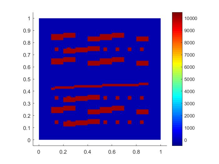 Figure 1
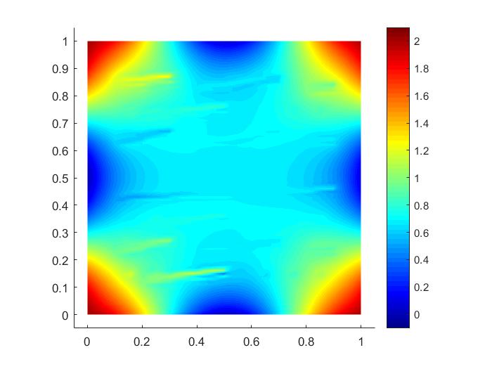 Figure 2
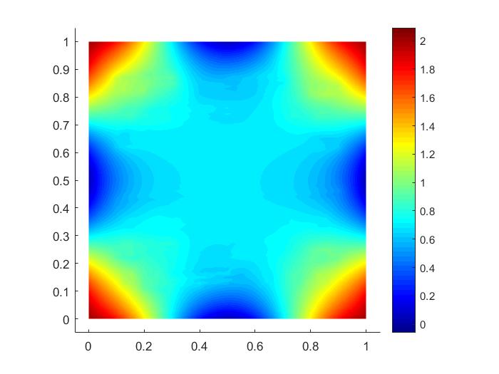 Figure 3
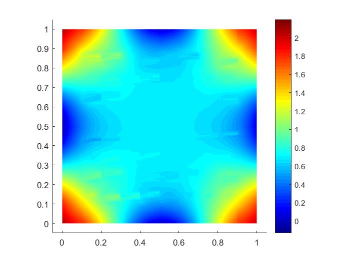 Figure 4
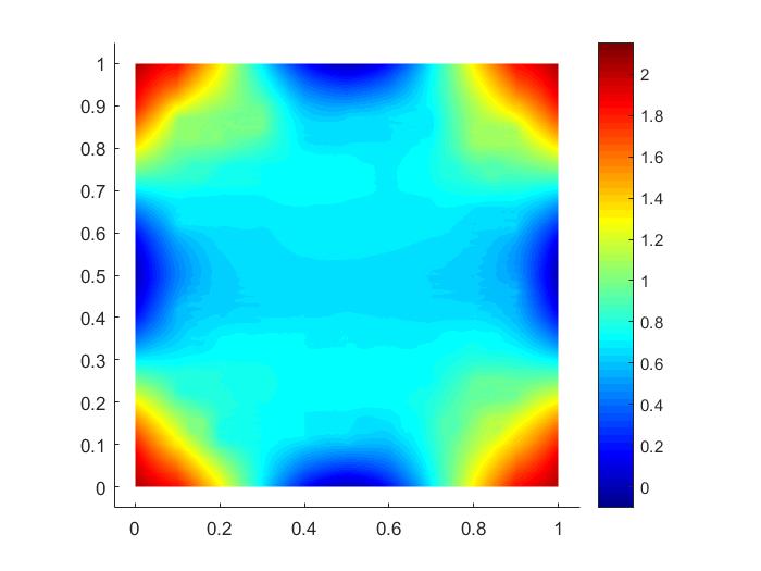 Figure 5
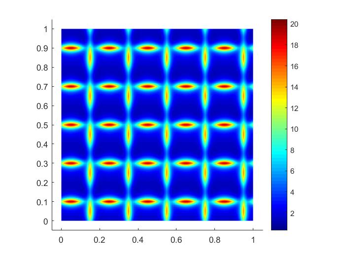 Figure 6
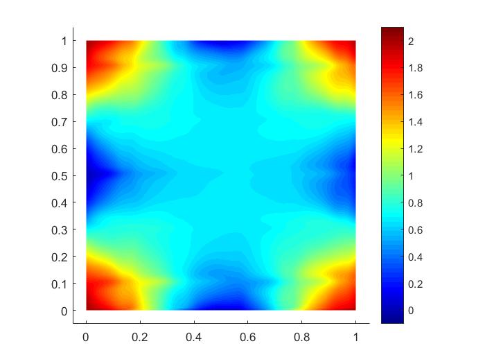 Figure 7
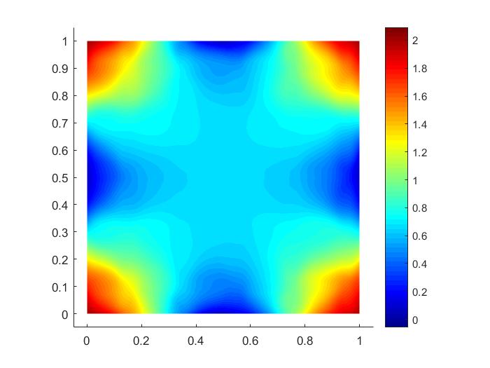 Figure 8
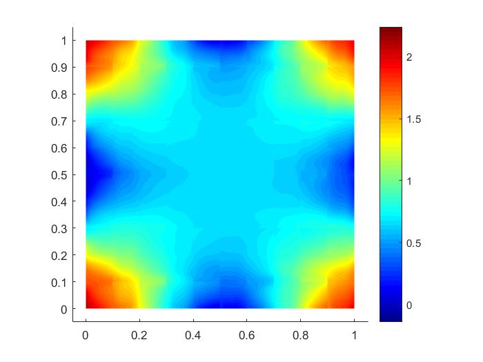 Figure 9
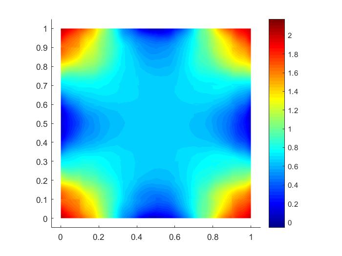 Figure 10
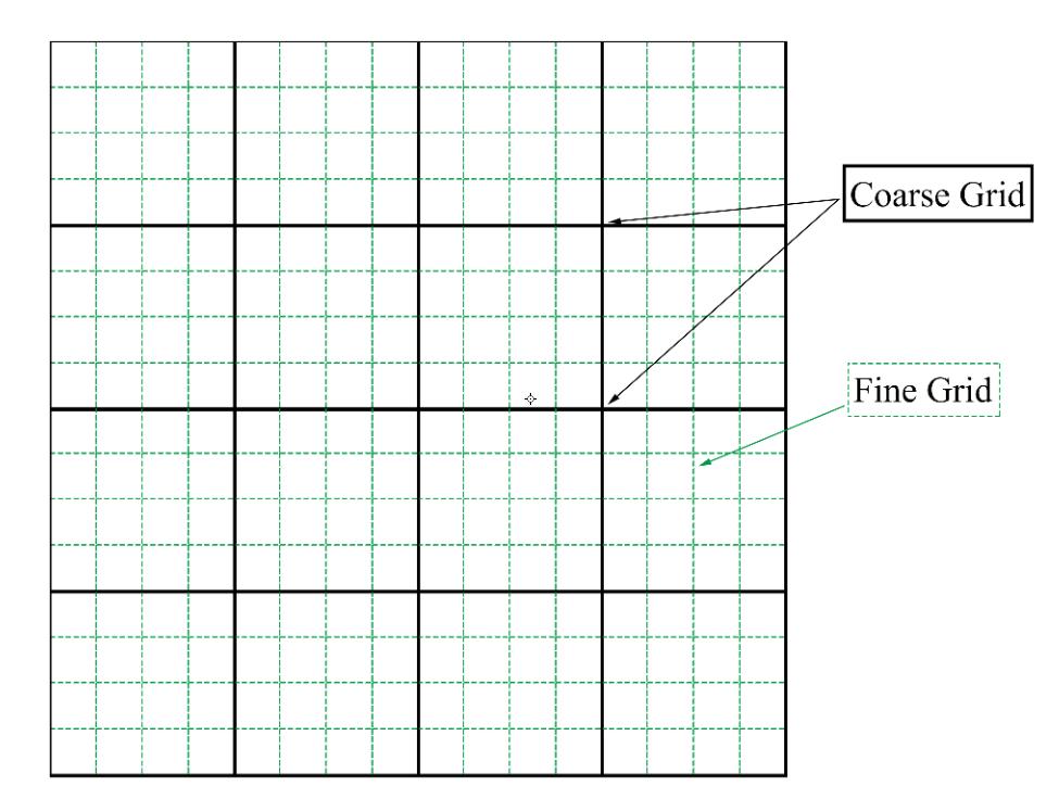 Figure 11
 Figure 12
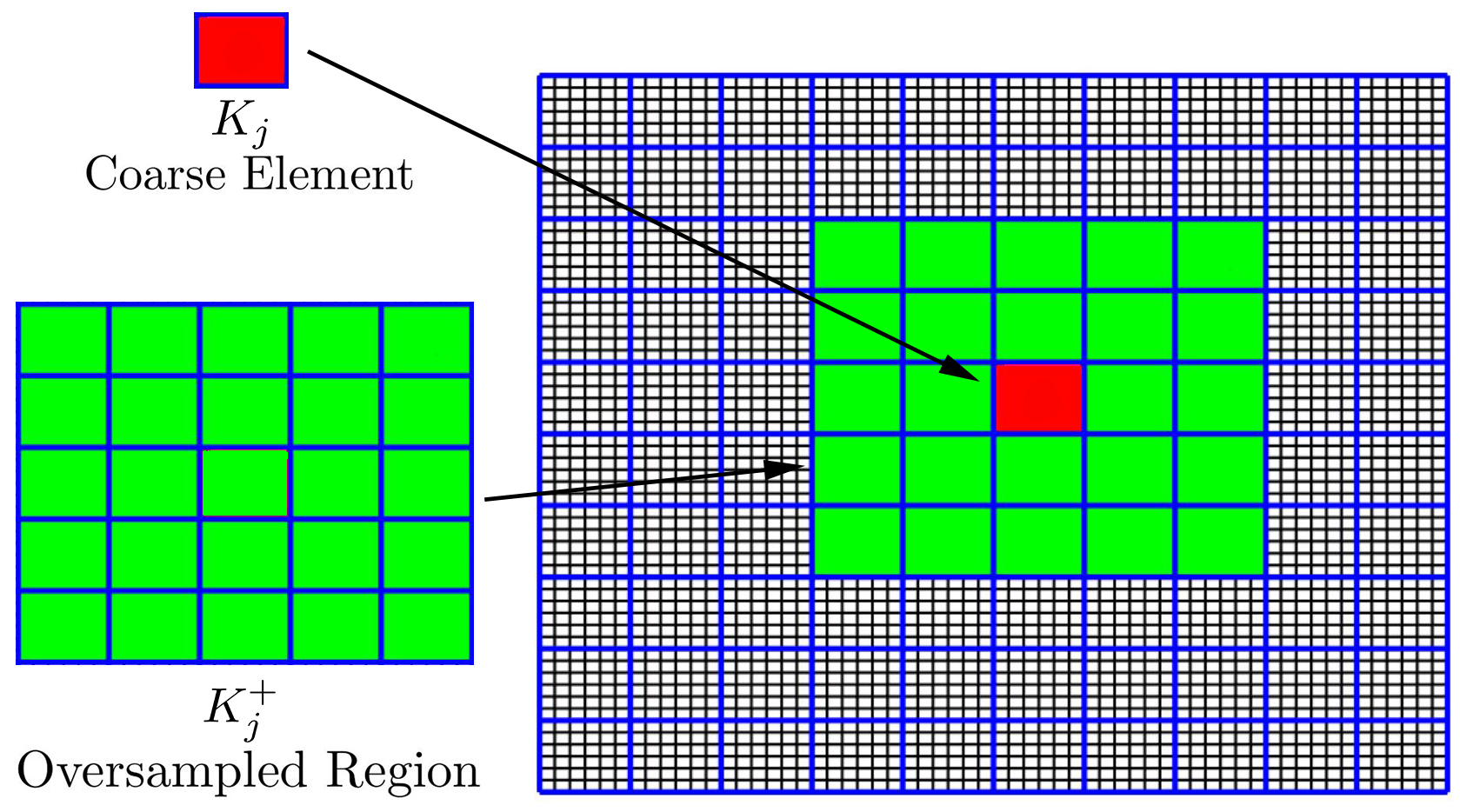 Figure 13
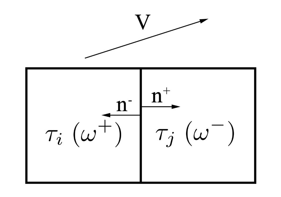 Figure 14
| snapshot ratio | |||
|---|---|---|---|
| 1 | 0.79% | 19.64% | 9.41% |
| 2 | 1.59% | 17.68% | 8.53% |
| 3 | 2.38% | 14.41% | 7.40% |
| 5 | 3.97% | 8.11% | 4.92% |
| 7 | 5.56% | 6.16% | 3.62% |
| 10 | 7.94% | 3.44% | 1.62% |
| 15 | 11.90% | 2.24% | 1.04% |
| 20 | 15.87% | 1.64% | 0.68% |
| snapshot ratio | |||
|---|---|---|---|
| 1 | 0.79% | 12.80% | 12.80% |
| 2 | 1.59% | 26.43% | 26.42% |
| 3 | 2.38% | 17.86% | 17.85% |
| 5 | 3.97% | 4.45% | 4.43% |
| 7 | 5.56% | 3.60% | 3.59% |
| 10 | 7.94% | 3.55% | 3.53% |
| 15 | 11.90% | 3.20% | 3.18% |
| 20 | 15.87% | 3.19% | 3.17% |
| snapshot ratio | |||
|---|---|---|---|
| 1 | 0.79% | 22.70% | 9.73% |
| 2 | 1.59% | 20.36% | 8.43% |
| 3 | 2.38% | 16.97% | 8.13% |
| 5 | 3.97% | 11.94% | 6.86% |
| 7 | 5.56% | 8.09% | 4.64% |
| 10 | 7.94% | 4.70% | 1.99% |
| 15 | 11.90% | 2.48% | 1.22% |
| 20 | 15.87% | 1.86% | 0.91% |
| snapshot ratio | |||
|---|---|---|---|
| 1 | 0.79% | 14.12% | 14.11% |
| 2 | 1.59% | 20.87% | 20.86% |
| 3 | 2.38% | 11.69% | 11.69% |
| 5 | 3.97% | 2.95% | 2.95% |
| 7 | 5.56% | 2.71% | 2.71% |
| 10 | 7.94% | 2.71% | 2.71% |
| 15 | 11.90% | 2.88% | 2.88% |
| 20 | 15.87% | 2.93% | 2.92% |
Peer Reviews
No public reviews on file for this paper yet. If you reviewed it on a platform where reviews are public (OpenReview, ICLR, NeurIPS, ICML), you can paste yours below so the community can read it here.
Videos
No videos yet. Explain this paper in a talk, walkthrough, or lecture? Add one.
Taxonomy
TopicsAdvanced Mathematical Modeling in Engineering · Composite Material Mechanics · Advanced Numerical Methods in Computational Mathematics
Generalized multiscale finite element method for the steady state linear Boltzmann equation
Eric Chung, Yalchin Efendiev, Yanbo Li and Qin Li Department of Mathematics, The Chinese University of Hong Kong, Hong Kong SAR. Email: [email protected] of Mathematics & Institute for Scientific Computation (ISC), Texas A&M University, College Station, Texas, USA. Email: [email protected] of Mathematics, Texas A&M University, College Station, Texas, USA. Email: [email protected] of Mathematics, University of Wisconsin, Madison, USA. Email: [email protected]
Abstract
The Boltzmann equation, as a model equation in statistical mechanics, is used to describe the statistical behavior of a large number of particles driven by the same physics laws. Depending on the media and the particles to be modeled, the equation has slightly different forms. In this article, we investigate a model Boltzmann equation with highly oscillatory media in the small Knudsen number regime, and study the numerical behavior of the Generalized Multi-scale Finite Element Method (GMsFEM) in the fluid regime when high oscillation in the media presents. The Generalized Multi-scale Finite Element Method (GMsFEM) is a general approach [7] to numerically treat equations with multi-scale structures. The method is divided into the offline and online steps. In the offline step, basis functions are prepared from a snapshot space via a well-designed generalized eigenvalue problem (GEP), and these basis functions are then utilized to patch up for a solution through DG formulation in the online step to incorporate specific boundary and source information. We prove the wellposedness of the method on the Boltzmann equation, and show that the GEP formulation provides a set of optimal basis functions that achieve spectral convergence. Such convergence is independent of the oscillation in the media, or the smallness of the Knudsen number, making it one of the few methods that simultaneously achieve numerical homogenization and asymptotic preserving properties across all scales of oscillations and the Knudsen number.
1 Introduction
The Boltzmann equation is a fundamental model in statistical mechanics. It traces the evolution of the distribution function on the phase space, and describes the dynamics of a large number of particles that follow the same physics rules via a statistical manner. The equation encodes the particles’ free transport and their interactions with the media and each other. Depending on the physics the particles follow, the interaction term may differ, but to a large extent, many particles, including neutrons, photons and phonons interact mainly with the media, making the collision term linear. The dynamics then can be described by the linear Boltzmann equation:
[TABLE]
In the equation, is a function on the phase space . The evolution is governed by , a free transport term, and the terms on the right side of the equation that represent the “collision” and quantify the particles’ interactions. These interactions include a pure absorption term where is the absorption coefficient, and a scattering term . The specific form of the operator varies from particle to particle, and it is typically a functional independent of . The strength of the interactions are governed by the size of and . For photons specifically, the radiative transfer equation is used, these coefficients are termed the optical thickness. In this paper, for simplicity, we take to be:
[TABLE]
where is a normalized measure: , and we set .
The equation demonstrates different behavior in different regimes. One particularly interesting regime is called the diffusion regime, in which the scattering coefficient is extremely strong and the pure absorption term is weak. Mathematically, consider the steady state case, we model the equation to:
[TABLE]
In this equation, is termed the Knudsen number, and it characterizes the ratio of the mean free path and the typical domain length. Physically it reflects the number of collision a normal particle experiences inside before emitting. When is small, the number of collision per particle is large, meaning the particle gets scattered many times before emitting, and thus some kind of averaging effects take place, and the local equilibrium is achieved. In the case of (2), the equilibrium reads:
[TABLE]
and through asymptotic analysis, one could mathematically derive that satisfies the diffusion equation:
[TABLE]
where depends on the dimension.
The convergence from (3) to the asymptotic limit (5) was conjectured in [4] and was made rigorous in [3] for periodic boundary condition. In [29] the authors studied the boundary layer effect with geometric corrections, and the asymptotic convergence rate was shown to degrade [26, 27].
However, all the rigorous proofs are done assuming certain smoothness of . In particular, it is assumed that is sufficiently smooth. At the current stage, very limited works have been done when oscillations present in the media. Denote the small scale in the media, we rewrite our equation as:
[TABLE]
where to explicit reflects the fast variable dependence. On the theoretical level, to our best knowledge, except a few cases [22], the theory is largely in lack, except a few cases [22], and to a large extend, we do not yet know the resonance of the two parameters, and how they contribute in the asymptotic limits of the equation. And on the computation level, the only numerical study aware to the authors is presented in [25] where the limits are taken in order: .
The problem is very challenging on the numerical level. The small makes the collision term extremely stiff, bringing ill-conditioning to the associated discrete system, and thus severe stability issue; and the small brings wild oscillations to the media and the solution, and for accuracy of the numerical solution, high resolution is needed and small discretization is necessary, driving up the numerical cost.
This is certainly unaffordable, especially in the zero limit of and . The main goal of this paper is to develop a general numerical treatment that could deal with the equation with a wide range of and , and perform uniformly well, with the error term independent on the small parameters.
The approach we take is in line of Generalized Multi-scale Finite Element Method (GMsFEM). This is an offline-online framework that builds a good set of local basis functions during the offline step and patches local solutions up in the online step, similar to the original Multi-scale Finite Element Method (MsFEM). One main feature of GMsFEM is its basis selection procedure in the offline step where a special generalized eigenvalue problem is designed. This special generalized eigenvalue problem encodes the oscillations and the ill-conditioning of the problem.
More explicitly, like many other multi-scale methods, we build nested grids with coarse grid and fine grid satisfying . In the offline step, local basis functions are constructed within coarse mesh on fine mesh that capture fine scale structure and preserve the heterogeneities in the media; and in the online step, the basis functions are patched up through Galerkin framework [2, 6, 17, 14, 15, 16, 20, 10, 11, 9, 19, 1, 24]. Online step is rather standard and different methods give various algorithms in the offline step. What makes GMsFEM favorable is indeed its offline step, in which the full list of -harmonic functions are collected, and then the most “representative” modes are selected through a specially designed generalized eigenvalue problem (GEP). The definition of the matrices in the GEP is associated with the final error term, which permits certain spectral error decay. We should mention GMsFEM was initially used for elliptic equations containing strong heterogeneous media, a topic about which the literature is extremely rich. For this particular problem, there is another category of method: upscaling-type methods. In upscaling methods, either locally or globally an effective media is numerically prepared so that equations could be computed on coarser grids with the effective media replacing the heterogeneous one [12, 30, 18, 21]. But this approach is not going to be pursued in this paper.
As a framework, the GMsFEM approach is rather easy to use, and the main mathematical challenge, when utilized for tackle different equations, is to develop the right GEP. For the linear Boltzmann equation with heterogeneous media, we frame the problem in the discontinuous Galerkin setting, and are able to find two matrices that resemble the mass and stiffness matrices in the GEP of the elliptic equations, which allows us to show the optimality of the basis functions with physically meaning definition of the norm for the error. As the standard approach, these basis functions are then used in the online computation.
The paper will be organized in the following way. In Section 2, we introduce some preliminaries. Both discrete ordinates, the standard kinetic solver, and GMsFEM for elliptic equation will be presented. Some properties will be presented along. We present the algorithm in Section 3, which is further divided into two subsection introducing offline and online procedures. Section 4 contains the analysis where we present the wellposedness, and convergence results. The small limit of the method will also be discussed. Numerical results are to be shown in Section 5.
To end the introduction, we comment that the scaling problem studied in this paper is not mathematically artificial. In fact, as one redefines , should have been automatically changed to highly oscillatory media . Another practical example is to inject light into crystals, where the radiative transfer equation (one particular linear Boltzmann equation) is utilized. In this case, the periodic crystal structure should be encoded in the media and the period that corresponds to in our math formulation, is expected to be small.
2 Preliminaries
In this section we prepare some basic important concepts. In particular, we will first present the discrete ordinate method for the linear Boltzmann equation, and then give a brief account of the Generalized Multiscale Finite Element Method (GMsFEM). They are the building blocks for the algorithm designed in this paper.
2.1 Boltzmann Equation
The Boltzmann equation gives a statistical description of particle dynamics. Its extensive use in all kinds of engineering problems brought its great popularity, and literature on both theory and numerics has been very rich. Among all numerical methods developed for the Boltzmann equation, the discrete ordinate method stands out for its simplicity and intuitiveness, and is the method we will use in our GMsFEM. Essentially it discretizes the velocity domain, and the semi-discrete system is a coupled PDE in the physical space.
We start the discussion with the following model equation:
[TABLE]
where is a bounded domain with a Lipschitz boundary . The velocity is , the unit circle. The media presents fine scale structure at order, and the stiffness of the collision operator is determined by . We have the inflow boundary condition, with the inflow data defined on , a collection of coordinates on the boundary with velocity pointing into the domain:
[TABLE]
Here is the unit outer normal direction at . For simplicity, we use the model collision operator with homogeneous scattering coefficient:
[TABLE]
The discrete ordinate method, denoted by , is a standard method to discretize the velocity domain. One first sample quadrature points on and each sample point is associated with a weight, denoted by: , where are the quadrature points and are the corresponding positive weights. These quadrature points and weights are chosen so that:
[TABLE]
The equation then will be discretized into semi-discrete system. Let , the integro-differential (7) is then transformed into a system of coupled partial differential equations:
[TABLE]
where is the inflow boundary data. Denote
[TABLE]
Then (9) is further simplified to:
[TABLE]
Since is basically the discrete version of the collision operator , it resembles the properties of . In particular, the matrix is positive semi-definite with a known kernel.
Proposition 1**.**
Define a matrix so that , we claim:
- •
* is positive semi-definite.*
- •
* if and only if is isotropic, i.e., .*
- •
* if either or is isotropic.*
Proof.
The computation is straightforward:
[TABLE]
The equal sign is achieved only when for all .
To show the third bullet point, we note that the matrix is symmetric, it suffices to assume that is isotropic: . Then:
[TABLE]
where we have used the weight condition (8): . ∎
2.2 Generalized Multi-scale Finite Element Method
The discrete ordinate method is used to discretize the velocity domain, and for the spatial domain, we follow the GMsFEM approach, which, by choosing “optimal basis functions” via a special design of a GEP, we can obtain a reduced model that is robust for all values of and . For the completeness of the paper, we now present a general idea of GMsFEM, and its application to the heterogeneous Boltzmann equation will be discussed in details in Section 3.
The GMsFEM uses two stages: offline and online. In the offline stage, a small dimensional approximation space is constructed to solve the global problem for any external source on a coarse grid, which does not need to resolve any scales of the media and solution. The offline stage consists of two main concepts. The snapshot space, , is constructed for a generic coarse element . The snapshot solutions are used to compute local multiscale basis functions. An appropriate snapshot space can
- •
provide a faster convergence,
- •
provide problem relevant restrictions on the coarse spaces (e.g., divergence free solutions),
- •
reduce the cost associated with constructing the offline spaces.
Standard choices of snapshot spaces (see [7]) are (1) all fine-grid functions; (2) snapshots of local solutions; (3) oversampling snapshots of local solutions; and (4) force-based snapshots. In this paper, we will use snapshots of local solutions.
More specifically, these are functions that satisfy
[TABLE]
subject to some boundary conditions, where is the differential operator under consideration, and is the index for the boundary condition. One can use all fine grid delta functions as boundary conditions or randomized boundary conditions [7, 5].
The offline space, , is computed for each (with elements of the space denoted ). We perform a spectral decomposition in the snapshot space and select the dominant eigenfunctions (corresponding to the smallest eigenvalues) to construct the offline (multiscale) space. The convergence rate of the resulting method is proportional to , where is the smallest eigenvalue that the corresponding eigenvector is not included in the multiscale space. We would like to select local spectral problem such that we can remove many small eigenvalues with fewer multiscale basis functions. The choice of spectral problems is usually problem dependent and is based on convergence analysis. In general, the error is decomposed into coarse subdomains. The energy functional corresponding to the domain is denoted by , e.g., . Then,
[TABLE]
where are coarse regions (), is the localization of the solution. The local spectral problem is chosen to bound . We seek the subspace such that for any , there exists with,
[TABLE]
where is an auxiliary bilinear form, and is an accuracy parameter. The auxiliary bilinear form needs to be chosen such that the solution is bounded in the corresponding norm.
Finally, in the online stage, the space is used together with a suitable coarse grid discretization to solve the problem. The same space is used for all input sources.
3 GMsFEM for heterogeneous Boltzmann equation
We now apply the GMsFEM approach to numerically study the heterogeneous Boltzmann equation, expressed in the discrete ordinate system (9).
The numerical difficulties in solving this equation are summarized as follows. First, the media is highly oscillatory. The fine structure oscillates at the scale of injects high heterogeneities to . In order to capture these details, the mesh size has to be smaller than , which in turn brings prohibitive numerical cost. Secondly, the operator is scaled by , and in the zero limit of , the term is extremely stiff, and this brings concern in stability. It is our aim in this paper to develop a multiscale method that can address these issues. In particular, inspired by GMsFEM, we will design a numerical method that relies on offline basis construction and online basis patching procedure, and its numerical error has limited dependence on the two small parameters.
We will construct nested grids and call the partition of into fine finite elements, and the partition into coarse elements, where and are the fine and coarse mesh sizes respectively. For simpler notation, we consider rectangular coarse elements as shown in Figure 1. The basis functions and discretization are based on the coarse grid, and the fine grid is used to numerically compute the basis functions. We also denote the collection of coarse edges , and the collection of coarse edges in the interior of the domain.
The discontinuous Galerkin method allows one to pick different values of the solution on different sides of the edges. Suppose two adjacent coarse blocks and share an edge, and that is the upwind block, then we denote and . Notice that depending on the direction of a specific , different block could be picked as the upwind block, as shown in Figure 2.
For the fine scale approximation, we choose the discrete function space to be:
[TABLE]
and we seek for numerical solution such that
[TABLE]
This means the numerical solution for each , when confined in each fine grid, is a linear function, and is continuous function across coarse grids. In the variational formulation: for all , we have:
[TABLE]
or with the definition of in (10), they could be summed up to
[TABLE]
In the equation, we have used upwind approximation for and the jump operator is defined by
[TABLE]
For notational simplicity, we define two bilinear operators
[TABLE]
and a linear operator:
[TABLE]
With these notations, equation (15) now writes
[TABLE]
With , it is a standard result that , with an error term of size . For significantly small , the function is considered as a reference solution in accessing the performance of our method.
However, using small that resolves and leads to a very big system that is numerically very costly. We would like to develop an algorithm that seeks for solution only on the coarse grid and the corresponding solution . To do that, an offline-online procedure developed in [5] for elliptic equation, termed GMsFEM (Generalized Multiscale Finite Element Method) will be pursued. In the offline step, an approximate space is constructed to replace . This newly constructed space would have much less degrees of freedom but preserves ’s important factors. The final multiscale solution will be computed in the online step where the boundary condition will be taken into account to determine the degrees of freedom in .
We quickly review the online stage in Section 3.1, and the complicated offline step will be discussed in detail in Section 3.2.
3.1 Online computation
In online stage, we will use the multiscale basis functions together with a coarse grid discretization to solve the given problem. The coarse grid discretization we used is a discontinuous Galerkin method with upwind flux. Assume that a multiscale finite element space is determined, and this space, in some sense, approximates . Then similar to the formulation as in (15), the solution will be sought in
[TABLE]
so that
[TABLE]
Similar to (16), we use a compact notation:
[TABLE]
To implement the scheme above, we define the following matrices
[TABLE]
Then the multiscale solution is formulated as
[TABLE]
where the coefficient vector solves .
3.2 Construction of
The key to the success of our method is the construction of the space on the coarse mesh during the offline stage. We will give the details here.
As discussed in Section 2.2, the offline step is further decomposed into two substages: constructing the snapshot space, and selecting modes associated with small eigenvalues. These two stages will be presented in Section 3.2.1 and Section 3.2.2 respectively.
In the snapshot space construction stage, in each coarse region, the Boltzmann solution will be solved multiple times together with all possible boundary conditions resolved by the fine grid. This give a high dimensional space. However, some modes in the snapshot space are more important than the others, and they dominate the numerical solution. To identify these basis functions, a specially designed local spectral problem (generalized eigenvalue problem GEP) is formulated and solved. The modes that correspond to the smallest eigenvalues are selected for form . The number of modes to be selected depends on the error tolerance and the eigenvalues of the GEP. The design of the local spectral problem is to encode the convergence error that is to be discussed in Section 4.
3.2.1 Snapshot Space
We present the construction of the snapshot spaces in this subsection. The procedure is the same in each coarse element, and we take the coarse element as an example. The snapshot space for this particular element is denoted by . We use the notation to denote the set of all nodes of the fine mesh lying in the upwind part of associated with velocity . And we also use to denote the union. Then the snapshot space is simply the linear span of solutions to the local Boltzmann equation with delta function as boundary condition, namely:
[TABLE]
where solves:
[TABLE]
Here we use multi-index Kronecker delta function , where is the standard basis in and is the standard Kronecker delta function:
[TABLE]
This strategy is summarized in Algorithm DetLocal.
The full snapshot space is given by
[TABLE]
Remark 1**.**
Numerically to prepare all snapshot basis functions is hard. It requires the computation of local Boltzmann equation with a large number of possible incoming delta functions. To reduce the cost of computation, we use the idea of oversampling [15]. To do so, the local computational domain is slightly enlarged to (see Figure 1), and a collection of random boundary condition is imposed on . The low rank structure of the solution space allows one to correctly capture the range, even with a limited sampling. In particular, we define the snapshot space
[TABLE]
where is the number of snapshot functions we could customize, and solves:
[TABLE]
where are random i.i.d. Gaussian sampling on . The solutions confined on are then used to form the snapshot spaces. We remark that the use of randomized boundary conditions on oversampling domains is able to reduce the offline computational cost as there is no need to impose delta function boundary conditions as in (24).
This strategy is summarized in Algorithm RanLocal.
Similar to (16) and (18), we can solve the snapshot solution by the following equation:
[TABLE]
We note that the snapshot solution can be considered as a reference solution. The error of the snapshot solution is related to the approximation property of the snapshot space in the fine scale space.
3.2.2 Offline Space
Now, we will present the construction of the solution space , with the property we mentioned in (13). In the end , when confined on each coarse element, say , will be a subspace of , and the construction of is amount to finding the most appropriate basis functions in to be included. The procedure is further divided into two sub-steps: the energy minimizing oversampling (EMO), and a design of a generalized eigenvalue problem, as used in [8].
We first denote the local oversampled snapshot space by . Notice that, for a given coarse element and its corresponding oversampling region , the space is the union of all snapshot spaces with the condition that .
Then the energy minimizing snapshots are calculated. For any snapshot function , its energy minimizing extension has the smallest energy in some norm and is sought in the local oversampled snapshot space with the constraint . In mathematical expression, for any , we seek for so that
[TABLE]
in which
[TABLE]
We notice that this construction is well-defined and the strategy is summarized in Algorithm EnergyMin. As one can see, is an extension of onto the oversampling domain that achieves the minimum energy, defined in (32) and this extension is crucial, as will be seen in the later analysis.
Remark 2**.**
This is about a stable decomposition property. It is important that the local basis functions satisfy a stable decomposition property. More precisely, the sum of local energies is bounded by the global energy.
Next, we define the two bilinear operators and , mentioned in (13). For simplicity of notation, we use and instead. For the element , define:
[TABLE]
Using the above bilinear forms, a spectral problem is defined. On , we look for such that
[TABLE]
where the eigenvalues are ordered in the ascending way:
[TABLE]
For implementation, we define the following matrices
[TABLE]
Then the pair is computed by solving
[TABLE]
Suppose modes are used for each . This strategy is summarized in Algorithm LocalGEP. The offline space is given by
[TABLE]
This will be the approximation space for solving the system (9) in the scheme (18).
3.3 Algorithm summary
We finally summarize the algorithm. Largely speaking, we prepare the basis functions in the offline step, and patch them up in the online step. The offline step is further divided into preparing a snapshot space in which either all Green’s functions are accumulated or a good random selection is obtained, and the basis selection step, in which the local generalized eigenvalue problem is computed and eigenfunctions with highest energies are chosen. These basis functions are ultimately used in the online step via the weak formulation (20). We summarize the procedure in Algorithm 1.
4 Analysis of the GMsFEM
In this section, we will present some analysis of our GMsFEM. In Section 4.1, we will prove the well-posedness of the discrete system resulting from the GMsFEM, and in Section 4.2, we will prove the convergence of the method. Finally, in Section 4.3, we will analyze the behavior of the method when is small.
4.1 Well-posedness
We first show the well-posedness of the GMsFEM (18).
Theorem 1**.**
Problem (18) has a unique solution, and the solution satisfies the following stability condition
[TABLE]
Proof.
Since the system (18) is a square linear system, showing the existence and uniqueness is amount to proving that for all only for trivial solution .
We will first prove the following inequalities
[TABLE]
First, is non-negative since the matrix is a positive semi-definite matrix, as discussed in Proposition 1. Next, the non-negativity of is shown below:
[TABLE]
Assuming for any , then setting , we have
[TABLE]
According to Proposition 1, we have
[TABLE]
meaning , and the solution to (18) is thus unique. For stability, we start with
[TABLE]
Considering , we conclude with the stability inequality (37). ∎
We notice that the snapshot equation (30) has the same structure, and the wellposedness is proved in the same way.
4.2 Convergence Analysis
We now analyze the convergence of the proposed method. The goal of this section is to estimate the difference between the snapshot solution, , computed in (30), and the multiscale coarse solution, , computed in (18). To do so, we first define the following norms. We define the -norm as:
[TABLE]
and -norm as:
[TABLE]
We also extend them by incorporating the collision term:
[TABLE]
The total energy is now defined by:
[TABLE]
Note that we have following propositions
Proposition 2**.**
* and *
Proof.
This proposition simply comes from the calculations in (38). ∎
Proposition 3**.**
If , we have
[TABLE]
Here and are bilinear operator defined in (33). where is the number of oversampled regions ’s which have nonempty intersection with coarse block , and is the number of oversampled regions ’s whose interior coarse edges contains coarse edge . They are both small numbers.
Proof.
We denote by . So . According to (31), has an energy minimizing extension that satisfies in . Then we have
[TABLE]
Combining with the definition of , we proved (44).
Next, we denote . By the definition of the energy minimizing extension in (31), we have
[TABLE]
Hence,
[TABLE]
and thus we have (45). ∎
For the convergence analysis, we first examine the best approximation property. For that, we have the following:
Lemma 1**.**
Let be the snapshot solution to the equation (30) and let be the multiscale solution to the equation (18). Then:
[TABLE]
where is a constant independent of , and the mesh size.
Proof.
Using (30) and (18), and the fact that , we have:
[TABLE]
Then for all :
[TABLE]
Using Proposition 2, we have:
[TABLE]
To obtain (46), noticing that and are both in , it amounts to show that:
[TABLE]
In fact it suffices to show that
[TABLE]
since it is obvious that .
To show (50), we first use integration by parts to obtain
[TABLE]
where we have used the continuity accross fine scales , and the assumption that, in each , satisfies the following equation
[TABLE]
for all . Here could be any function in restricted on . In particular, (51) works for .
Using the definition of and direct calculations, we have
[TABLE]
Then, applying the Cauchy-Schwarz inequality, we have
[TABLE]
The two terms on the right hand side are taken care of separately. To handle the first term, recall the definition of -norm in equation (41), we have
[TABLE]
And to compute the second term, we notice that
[TABLE]
which in turn gives
[TABLE]
Plug (53) and (4.2) into (4.2), we have proved the desired boundedness condition (50) which concludes the proof of (46). ∎
Now, we are ready to prove our main convergence result in this section.
Theorem 2**.**
Let be the snapshot solution to problem (30) and let be the multiscale solution to problem (18). Then:
[TABLE]
where , is the same constant from Lemma 1, and is the same constant from Proposition 3.
Proof.
We first denote
[TABLE]
where is the -th multiscale basis function for the coarse element (35). Note that covers the entire snapshot space. We then define a projection of into , as well as a projection of into :
[TABLE]
It is easy to see that . Combining with Proposition 3, we have
[TABLE]
Combining with Lemma 1, we proved the theorem. ∎
In the above theorem, we estimate the error between the snapshot solution and the multiscale solution . We see that the error is inversely proportional to the eigenvalues. This shows that the multiscale space gives a good approximation property in the snapshot space. In our analysis, we assume that the snapshot functions satisfy the PDE in the strong sense, that is, (51). On the other hand, there is an error between the snapshot solution and the fine scale solution if we use Algorithm RanLocal in Section 3.2. This amounts to an irreducible error, and the analysis of this is beyond the scope of this paper.
We should emphasize that the difficulty brought by small is encoded in the quality of and thus is not explicitly expressed in the error analysis.
4.3 Small regime
An important property the algorithm satisfies is that it is robust with respect to the parameters. In the limiting regime of , has a positive lower bound, and this serves as the stability argument that allows the algorithm to be effective across regimes. In particular we will show:
Theorem 3**.**
Denote the -th eigenvalue of the GEP defined in (35) for coarse element . It has a asymptotic limit in the zero limit of , meaning there is a constant so that:
[TABLE]
This theorem, when combined with our main Theorem 2, indicates that the error bound, which is controlled by , will not grow in and thus the error is uniformly bounded.
To show the theorem, we first start with a lemma.
Lemma 2**.**
For every coarse element , we have
[TABLE]
where entries in and are defined by:
[TABLE]
and
[TABLE]
where , and is the basis functions’ energy minimizing extension. We further denote the leading order asymptotic expansion of .
Proof.
To proceed we notice that can be written as the sum of some ’s, where and . Recall the assumption of equation (51). Then in each and for all , we have:
[TABLE]
Here could be any function in restricted on .
Therefore we have:
[TABLE]
Take the asymptotic expansion for :
[TABLE]
set , and plug them back into (58). We have, in the leading order of :
[TABLE]
meaning is isotropic in each due to Proposition 1. Therefore is isotropic. The same analysis is applied to .
Recall the definition of and in (33), we have:
[TABLE]
Due to Proposition 1, we have:
[TABLE]
and thus
[TABLE]
The proof for is the same and is omitted here. ∎
Theorem 3 is straightforward consequence of the following perturbation theorem:
Proof for Theorem 3.
According to Lemma 2, and have expansions and . We also define as the -th generalized eigenvector of the two matrices and , i.e.
[TABLE]
Using Absolute Weyl theorem for generalized eigenvalue problems in [28], when is small enough such that , we have:
[TABLE]
where is the spectral norm of a matrix. ∎
According to the formula for and in (55) and (56), the eigenvalues are positive except that the smallest one is 0 with constant as corresponding eigenvector. So has positive limit in the limiting regime of .
5 Numerical results
We take boundary condition . And we set , and use Gaussian quadrature rule to define . As for , we give two examples. In the first example, we will choose to be based on a high contrast media , shown in Figure 3(Left), and choose to be an oscillatory function for the second example used in [25, 13, 23], shown in Figure 3(Right), with expression
[TABLE]
The space domain is taken as the unit square and is divided into coarse blocks consisting of uniform squares. Each coarse element is then divided into fine elements consisting of uniform squares. That is, is partitioned by square fine elements. And we use oversampling technique in equation (26)-(29) to obtain the snapshot space. We define an oversampling region by enlarging by one coarse grid layer.
To compare the accuracy, we will use the following error quantities:
[TABLE]
where is defined as
For Example 1, we first fix and give the error tables for Knudsen number , respectively. And is the number of multiscale basis chosen from each coarse element, and snapshot ratio is define by
[TABLE]
From Table 2, 2, 4, we can see this framework works for all Knudsen number , which verifies our proved conclusion. In addition, we see clearly the reduction of error when more basis functions are used, and the reduction of error is more rapid when fewer basis functions are used. We also observe that the method gives reasonable error levels with small snapshot ratios. On the other hand, Figures 4 show the fine and multiscale solutions with and . From these figures, we observe very good agreements between the fine-scale and multiscale solutions
Next, we fix and change the high contrast value of . We set , respectively. From Table 4, we can see that contrast values do not affect the error.
For Example 2, we give the error tables for , respectively. We present the errors for using various choices of number of basis functions in Table 6, 6, 7. We clearly see that, with a very small snapshot ratio, our method is able to obtain solutions with very good accuracy. Furthermore, we observe a faster decay of the error when smaller number of basis functions are used. In Figures 5, we present the fine and multiscale solutions with and . We observe very good agreement of both solutions.
Acknowledgements
Q. L.’s research is supported by NSF-DMS 1619778, 1750488, and UW-Madison Data Science Initiative. E. C.’s research is partially supported by Hong Kong RGC General Research Fund (Projects 14304217 and 14302018) and CUHK Direct Grant for Research 2018-19.
The reference list from the paper itself. Each links out to its DOI / PubMed record.
- 1[1] J.E. Aarnes. On the use of a mixed multiscale finite element method for greater flexibility and increased speed or improved accuracy in reservoir simulation. SIAM J. Multiscale Modeling and Simulation , 2:421–439, 2004.
- 2[2] Todd Arbogast. Analysis of a two-scale, locally conservative subgrid upscaling for elliptic problems. SIAM Journal on Numerical Analysis , 42(2):576–598, 2004.
- 3[3] Claude Bardos, Rafael Santos, and Rémi Sentis. Diffusion approximation and computation of the critical size. Transactions of the american mathematical society , 284(2):617–649, 1984.
- 4[4] Alain Bensoussan, Jacques-Louis Lions, and George Papanicolaou. Asymptotic analysis for periodic structures , volume 374. American Mathematical Soc., 2011.
- 5[5] V. Calo, Y. Efendiev, J. Galvis, and G. Li. Randomized oversampling for generalized multiscale finite element methods. ar Xiv preprint, ar Xiv: 1409.7114 , 2014.
- 6[6] C-C Chu, Ivan Graham, and T-Y Hou. A new multiscale finite element method for high-contrast elliptic interface problems. Mathematics of Computation , 79(272):1915–1955, 2010.
- 7[7] Eric Chung, Yalchin Efendiev, and Thomas Y Hou. Adaptive multiscale model reduction with generalized multiscale finite element methods. Journal of Computational Physics , 320:69–95, 2016.
- 8[8] Eric Chung, Yalchin Efendiev, and Wing Tat Leung. Generalized multiscale finite element methods with energy minimizing oversampling. International Journal for Numerical Methods in Engineering , 117(3):316–343, 2019.