A decorated tree approach to random permutations in substitution-closed classes
Jacopo Borga, Mathilde Bouvel, Valentin F\'eray, Benedikt Stufler

TL;DR
This paper introduces a new bijective encoding of permutations as decorated trees, enabling analysis of their local and global limits within substitution-closed classes, and strengthening existing permuton limit results.
Contribution
It presents a novel bijective encoding of permutations as decorated trees and applies it to prove local convergence and enhance permuton limit results for substitution-closed classes.
Findings
Established local convergence of uniform random permutations in certain classes
Reproved and strengthened permuton limit results using new methods
Connected permutation limits with size-constrained Galton-Watson trees
Abstract
We establish a novel bijective encoding that represents permutations as forests of decorated (or enriched) trees. This allows us to prove local convergence of uniform random permutations from substitution-closed classes satisfying a criticality constraint. It also enables us to reprove and strengthen permuton limits for these classes in a new way, that uses a semi-local version of Aldous' skeleton decomposition for size-constrained Galton--Watson trees.
Click any figure to enlarge with its caption.
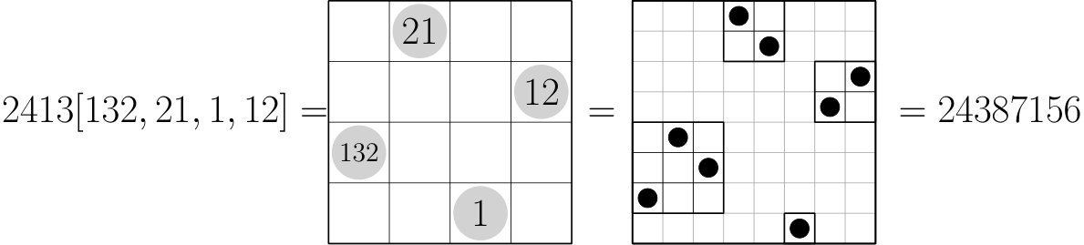 Figure 1
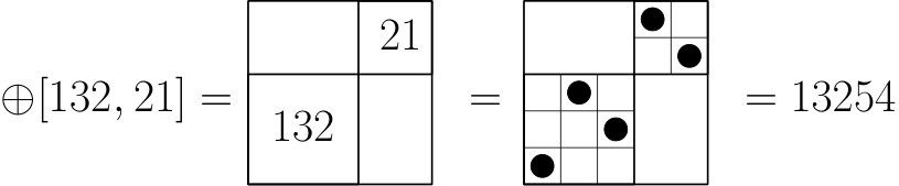 Figure 2
 Figure 3
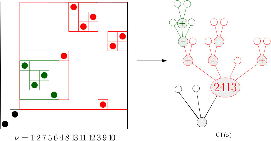 Figure 4
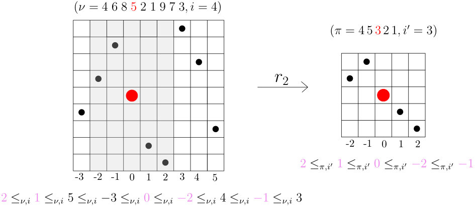 Figure 5
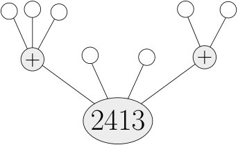 Figure 6
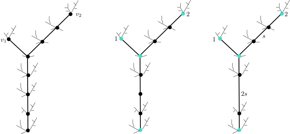 Figure 7
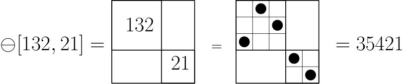 Figure 8
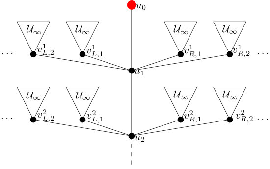 Figure 9
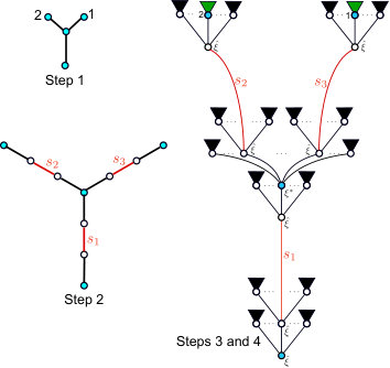 Figure 10
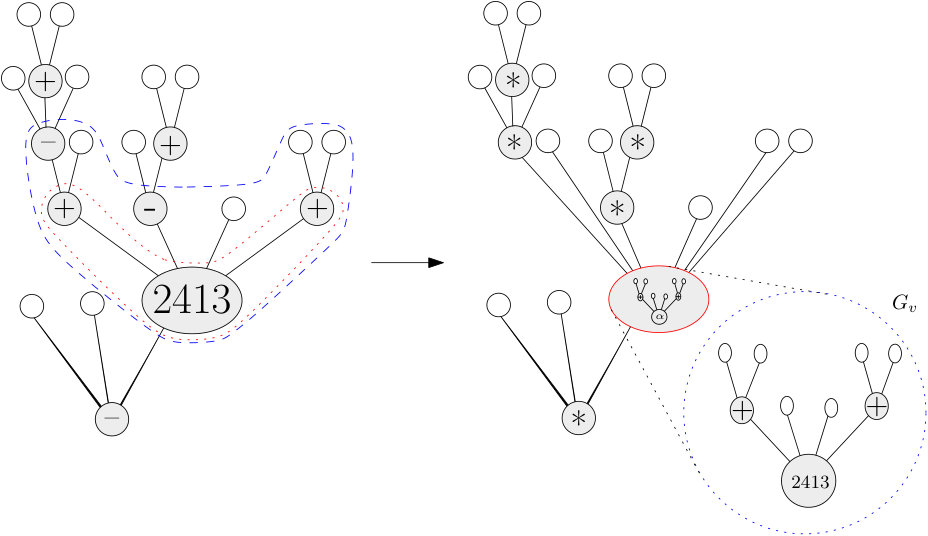 Figure 11
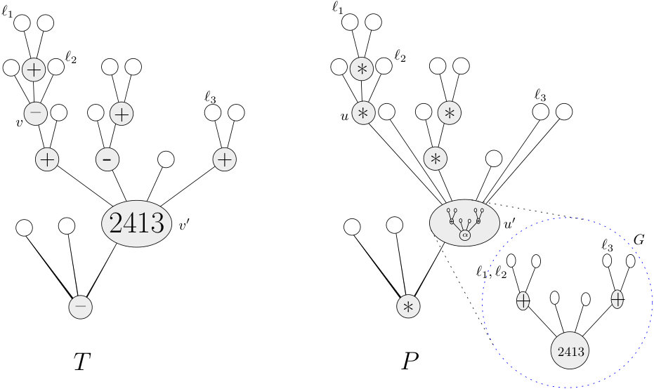 Figure 12
| the set of permutations of size page 1.8 | |
| a substitution-closed class of permutations, page 2.10 | |
| the subset of simple permutations in , page 2.11 | |
| the class of canonical trees associated with , page 2.3 | |
| the class of packed trees associated with , page 2.20 | |
| the uniform random -sized permutation from , page 3 | |
| the uniform random packed tree with leaves, page 3.4 | |
| the collection of (possibly infinite) pointed plane trees, page 6.6 | |
| the collection of (possibly infinite) locally and upwards finite | |
| pointed plane trees, page 6.6 | |
| the collection of (possibly infinite) locally and upwards finite | |
| decorated pointed plane trees, page 6.6 | |
| the collection of (possibly infinite) locally and upwards finite | |
| pointed packed trees, page 6.3 |
Peer Reviews
No public reviews on file for this paper yet. If you reviewed it on a platform where reviews are public (OpenReview, ICLR, NeurIPS, ICML), you can paste yours below so the community can read it here.
Videos
No videos yet. Explain this paper in a talk, walkthrough, or lecture? Add one.
\SHORTTITLE
A decorated tree approach to random permutations in substitution-closed classes \TITLEA decorated tree approach to random permutations in substitution-closed classes \AUTHORSJacopo Borga111Institut für Mathematik, Universität Zürich. \[email protected] and Mathilde Bouvel222Institut für Mathematik, Universität Zürich. \[email protected] and Valentin Féray333Institut für Mathematik, Universität Zürich. \[email protected] and Benedikt Stufler444Institut für Mathematik, Universität München. \[email protected]
\KEYWORDSpermutation patterns, local and scaling limits, Galton–Watson trees \AMSSUBJ60C05,05A05 \SUBMITTEDApril 15, 2019 \ACCEPTEDMay 26, 2020 \ARXIVID1904.07135 \VOLUME0 \YEAR2016 \PAPERNUM0 \DOI10.1214/YY-TN \ABSTRACTWe establish a novel bijective encoding that represents permutations as forests of decorated (or enriched) trees. This allows us to prove local convergence of uniform random permutations from substitution-closed classes satisfying a criticality constraint. It also enables us to reprove and strengthen permuton limits for these classes in a new way, that uses a semi-local version of Aldous’ skeleton decomposition for size-constrained Galton–Watson trees.
1 Introduction
1.1 Uniform random permutations in classes: some background and overview of our results
We assume some familiarity of the reader with basic definitions of permutation patterns and permutation classes, i.e., what is a pattern, an occurrence and a consecutive occurrence, a class, its basis, … If needed, the definitions of these notions are given at the end of the introduction.
Permutation classes are classically studied from an enumerative point of view, i.e., one wants to compute the number of permutations of any fixed size in a given class or the generating function of the class (possibly refining according to some statistics). In recent years, there has also been an increasing interest in the behaviour of a large typical permutation taken in a given permutation class. We refer for example to [13, 24, 25, 26, 32, 33, 43, 44] for results on random -avoiding permutations with of size . Other specific classes (or sets of permutations) have been studied: permutations avoiding a monotone pattern of any size [27], separable permutations [9], square permutations [14, 15], doubly alternating Baxter permutations [20]. The recent paper [7] by Bassino, Bouvel, Féray, Gerin, and Maazoun uses singularity analysis methods to study random permutations from substitution-closed classes satisfying some analytic assumptions.
The present work takes a probabilistic approach to the analysis of random permutations from substitution-closed classes. We establish a novel encoding of these permutations as decorated conditioned monotype Galton–Watson forests, hence integrating them into the framework of random enriched trees and tree-like structures introduced by Stufler [48, 50]. This yields a unified and powerful way for describing their asymptotic shape on a global and local scale.
- •
As a first application we give a new proof of the main scaling limit result of [7, 9] by using an extension of Aldous’ skeleton decomposition (see [6] for Aldous’ original statement, and Lemma 4.3 for our extension). This new proof works under weaker conditions and makes transparent the connection to random trees which was suggested, but unclear, in [7] (see in particular Remark 1.11 or the beginning of Section 1.7 there). In particular, our proof yields a probabilistic interpretation of the conditions under which this scaling limit result holds (see Section 1.6).
- •
Our second main contribution is a novel quenched local limit for random permutations from substitution-closed classes. Here we use fringe subtree count asymptotics and the skeleton decomposition to describe a concentration phenomenon for consecutive patterns. This notion of convergence has recently been introduced by Borga in [13], where such limits were proven for random permutations avoiding patterns of length .
The rest of the introduction defines substitution-closed classes and provides details on our results and on the approach used in this paper.
1.2 Substitution of permutations and closed classes
To define the substitution operation, it is convenient to think of permutations as diagrams. That is, if denotes the size of a permutation , we may identify with the set of points (for in ). The substitution , where are permutations and is the size of , is then obtained as follows. For each , we first replace the point with the diagram of . Then rescaling the rows and columns yields the diagram of a bigger permutation, which is by definition . A permutation of size greater than is called simple if it cannot be obtained as the substitution of smaller permutations. An example of substitution is given in Fig. 1.
As said above, this article considers substitution-closed classes of permutations, i.e., classes such that implies . Alternatively, a class is substitution-closed if and only if its basis (i.e., the avoided patterns defining the class) consists only of simple permutations. In particular, there are uncountably many substitution-closed permutation classes. Due to their nice combinatorial structure (see Section 2), substitution-closed permutation classes are a nice general framework, where to investigate the properties of uniform random elements.
We note that a substitution-closed class is entirely determined by the set of simple permutations in it (see Proposition 2.11). We consider this set as the data of our problem, and the goal is, under various conditions on to obtain convergence results for uniform random permutations in the class . These conditions will typically be expressed in terms of the generating functions of , that we conveniently also denote . From Stanley-Wilf-Marcus-Tardös’ theorem [41], it always has a positive radius of convergence (except in the trivial case where is the set of all permutations, which we exclude from now on; permutation classes different from are called proper).
1.3 Permuton convergence of substitution-closed classes
The notion of permutons was introduced in [29] to describe limits of permutation sequences. Formally, a permuton is a probability measure on the unit square , whose projection on each axis is the Lebesgue measure on (we say that the measure has uniform marginals). Permutations can be seen as permutons by considering the rescaled diagrams; we will denote the permuton associated with the permutation . The weak topology on measures gives then a natural meaning to the convergence of a sequence of permutations to a given permuton. A nice feature is that the convergence in terms of permutons is equivalent to the convergence of pattern proportions. We refer to [7, Section 2] for details.
Some specific permutons have been described as limits of permutation classes, as in [12, Chapter 6], [15] and [9, 7, 8]. Among these, the biased Brownian separable permuton of parameter is a random permuton, constructed from a Brownian excursion and independent signs associated with its local minima, see Maazoun [40]. It was proved in [7, 9] that this is a universal limiting object for substitution-closed permutations classes, in the sense that uniform random permutations in many substitution-closed classes converge to , for some . In this article, we give a new proof of this theorem that is based on an extension of Aldous’ skeleton decomposition [6] and the framework of random enriched trees and tree-like structures [48, 50].
Theorem 1.1**.**
Let be the uniform -sized permutation from a proper substitution-closed class of permutations . Suppose that
[TABLE]
or
[TABLE]
Then
[TABLE]
with denoting the biased Brownian separable permuton with an explicit parameter given by Eq. 45 page 45. This includes the case of uniform separable permutations, for which and .
Specifically, the result [9, Thm. 1.2] corresponds to the special case where , and [7, Thm. 1.10] corresponds to the special case where Eq. 1 is satisfied. The result [7, Thm. 7.8] corresponds to the case where Eq. 2 is satisfied and additionally is amendable to singularity analysis.
1.4 Local convergence: a concentration phenomenon for substitution-closed classes
In addition to scaling limits, our decorated tree approach also allows us to obtain local limit results for uniform random permutations in substitution-closed classes. For this, we use a local topology for permutations recently defined by Borga in [13]. This topology is the analogue of the celebrated Benjamini–Schramm convergence for graphs, in the sense that we look at the neighbourhood of a random element of the permutation. Pleasantly, convergence for this local topology is equivalent to the convergence of consecutive pattern proportions.
For convenience, we present our results in term of consecutive patterns. For a permutation and a pattern , we denote by the number of consecutive occurrences of a pattern in ; for instance, for (resp. ), these are the number of descents (resp. double-descents) in the permutation.
Theorem 1.2**.**
Let be a proper substitution-closed permutation class and assume that
[TABLE]
For each , we consider a uniform random permutation of size in . Then, for each pattern , there exists in such that
[TABLE]
We note that the hypothesis made in this theorem is slightly weaker than that for scaling limits. The theorem shows the convergence of all random variables to deterministic constants, revealing a "concentration" phenomenon in substitution-closed class under hypothesis (3). The constants can be constructed from local limits of conditioned Galton–Watson trees around a random leaf, see Section 6 and in particular Remark 6.30. They depend both on the pattern and on the class .
1.5 Proof methodology
Start with a permutation of size . If it is not simple nor monotone555By definition, for , there are exactly two monotone permutations of size : the monotone increasing one and the monotone decreasing one ., it can be written as , for some smaller permutations . We can iterate this decomposition on : as long as they are not simple nor monotone, we decompose them further through substitution. The result is a representation of as a tree with leaves, whose internal vertices are decorated by monotone or simple permutations. We call positive (resp. negative) a decoration with a monotone increasing (resp. decreasing) permutation. From a result of Albert and Atkinson [2], the decorated tree representation of a permutation is unique if we forbid the children of a vertex with a positive (resp. negative) decoration to have themselves a positive (resp. negative) decoration. The resulting tree is called the canonical tree of the permutation. Details on this construction, standard in the permutation pattern literature, are given in Section 2.2.
From a probabilistic point of view, one wants to consider the tree associated with a uniform random permutation in a class and possibly to recognize some standard tree models. One can show that, if the class is substitution-closed, the associated random canonical tree is a multitype random Galton–Watson tree with some specific offspring distribution conditioned on having leaves. The need to have several types comes from the condition on positive and negative decorations: this forces us to consider children of positively and negatively decorated vertices to be of a different type from other vertices in the tree.
Results on conditioned multitype Galton–Watson trees do exist in the literature: in particular, there are some scaling limit results under finite or infinite variance assumptions [11, 18, 42], and local limit results around the root [1, 47] for such trees. Nevertheless these results do not cover our needs.
- •
For the scaling limit results on permutations, we need information on the type and outdegree of the closest common ancestors of randomly selected leaves (while tree scaling limit results only give information on the genealogy of such leaves).
- •
For the local limit results on permutations, we need some local limit results around a random leaf, and not around the root. For studying local convergence of random separable permutations we additionally require joint convergence with the parity of the height of the leaf.
We therefore do not use this encoding as multitype Galton–Watson trees, but rather provide a novel encoding of random permutations in substitution-closed classes as decorated monotype Galton–Watson forests. That is, random plane forests where each vertex is enriched with an independent local structure. This integrates the random permutations naturally into the framework of random tree-like structures [48].
To identify permutations with decorated forests, we first note that a generic permutation is the -sum of an ordered sequence of -indecomposable permutations, i.e., of permutations which cannot be obtained as a substitution (see Theorem 2.5 below). We then associate to each of these -indecomposable permutations its canonical tree. To those trees, we apply a packing procedure. This packing procedure merges vertices decorated with a simple permutation with its children having a positive decoration. As a consequence, we do not need anymore to distinguish between positive and negative decorations. The resulting tree, called packed tree of the (-indecomposable) permutation, is still a decorated tree with leaves, but the decorations are now more complicated objects than permutations, being themselves trees of permutations (called -gadget below, see Section 2.3 for details). The advantage of this new representation is that there is no condition on the decoration of a vertex, depending on the one of its parent. As a result of this construction, any permutation is represented as an ordered sequence of decorated trees, i.e., an ordered decorated forest, without any constraint on the decorations (Theorem 2.21). We note that this representation is a bijection from the set of all permutations to ordered decorated forests, and could thus be of interest, independently from its application to the study of random elements in substitution-closed classes done here.
To study random permutations of size taken uniformly at random in a substitution-closed class , we use a result on convergent Gibbs partitions (see Stufler [49, Thm. 3.1]) to prove that the associated ordered decorated forest contains a giant tree of size (Proposition 3.2 page 3.2). It is therefore enough to study a random decorated tree with leaves. Such trees have the same distribution as a monotype Galton–Watson tree with a specific offspring distribution conditioned on having leaves. We can therefore use results or techniques on monotype Galton–Watson trees, which are much more developed than in the multitype case.
- •
In particular, to find the scaling limit of our permutations, there are some results on the genealogy and the outdegree of common ancestors of randomly chosen vertices (this is implicit in the original paper of Aldous, see [6, Eq. (49)]). We will refer to this as Aldous’ skeleton decomposition. In this article we will need an extension of this, considering also local neighbourhood of the common ancestors (being therefore semi-local) and allowing to condition on the number of leaves instead of the number of vertices. Lemma 4.3 provides a general result to this effect, allowing to condition on the number of vertices with arity in any given set satisfying .
- •
The literature also contains results on the number of (extended) fringe subtrees of (and related models) isomorphic to a given tree [3, 28, 31, 48, 51, 52]. When is critical, such results may be translated to local limit results for , pointed at a random leaf (see Proposition 6.13). We shall however need and will prove a slightly stronger result when is critical and additionally has finite variance, taking also into account the parity of the height of the pointed leaf (see Proposition 6.25 page 6.25).
The last step of the proofs (both in the scaling and local limit cases) is to translate the results on the packed trees to results on the permutation itself. A difficulty here arises from the identification of positive and negative decorations in the packing construction. To invert this construction, and recover the correct signs on the decorated trees, we need to determine the distance to the closest ancestor decorated with a simple permutation. When , this ancestor is at a stochastically bounded distance, so that this inversion procedure is still local. However, when , i.e., in the case of separable permutations, there is no such ancestor and we need to go all the way to the root to invert the packing construction. This creates an extra difficulty, that we overcome by using a local limit theorem for the length of “bones” in the skeleton decomposition.
1.6 Interpretation of the various assumptions on
Our assumptions on might seem artificial but they are in fact very natural, after having introduced the above representation of permutations as decorated conditioned Galton–Watson forests. Namely
- •
Eq. 3 is equivalent to the fact that the Galton–Watson tree model is critical;
- •
Eq. 1 asks in addition that the offspring distribution has small exponential moments;
- •
finally, Eq. 2 means that the offspring distribution has no exponential moments, but finite variance.
Such hypotheses are classical in the analysis of conditioned Galton–Watson trees, and give a probabilistic meaning to the conditions used in [7]. In terms of substitution-closed classes, the small exponential moment condition is satisfied for most classes in the literature, see the discussion in [7, Section 1.4]. Although general classes satisfying Eq. 3 but not Eq. 1 have also been studied in previous works [7, Sec. 7], we do not know at present whether such classes exist.
There is however at least one class not satisfying Eq. 3: the class . The packed forest associated with a uniform random permutation in this class has the distribution of a decorated conditioned Galton–Watson forest with a subcritical offspring distribution. It will therefore contain with high probability a unique vertex with macroscopic degree (see [31, 34, 38, 52]). This vertex is decorated with a large simple permutation in the class and the scaling (resp. local) limit of could be described if one knew that of . In the current state of the art, studying a uniform random simple in does not seem to be a simpler problem than the original one of studying , hence this approach appears to be ineffective for .
1.7 Outline of the paper
The paper is organized as follows. The rest of the introduction sets up some notation. Section 2 presents the combinatorial construction used in this paper, that is the canonical tree and packed forest associated with a permutation. Section 3 identifies the packed forest associated with a uniform random permutation in a substitution-closed class as a conditioned monotype Galton–Watson forest. We also discuss the existence of a giant tree in such a forest. In Section 4, we state and prove our improvement of Aldous’ skeleton decomposition. The last two sections are devoted to the proofs of the main theorems: Section 5 for the scaling limit result (Theorem 1.1) and Section 6 for the local limit result (Theorem 1.2).
1.8 Permutation patterns and permutation classes: basic definitions and notation
We let denote the collection of non-negative integers and the collection of strictly positive integers. For any we denote the set of permutations of by We write permutations of in one-line notation as For a permutation the size of is denoted by We let be the set of finite permutations. We write sequences of permutations in as
We will often view a permutation as its diagram, which is (as said earlier – see also the right part of Fig. 1) the set of points of the Cartesian plane at coordinates .
If is a sequence of distinct numbers, let be the unique permutation in that is in the same relative order as i.e., if and only if Given a permutation and a subset of indices , let be the permutation induced by namely, \text{pat}_{I}(\nu)\coloneqq\text{std}\big{(}(\nu(i))_{i\in I}\big{)}. For example, if and then .
Given two permutations, for some and for some we say that contains as a pattern (and we write ) if has a subsequence of entries order-isomorphic to that is, if there exists a subset such that . Denoting the elements of in increasing order, the subsequence is called an occurrence of in . In addition, we say that contains as a consecutive pattern if has a subsequence of adjacent entries order-isomorphic to , that is, if there exists an interval such that . Using the same notation as above, is then called a consecutive occurrence of in . All along the article, for any integers (resp. ), the interval (any interval ) is to be understood as an integer interval, i.e., an interval contained in . For real numbers , we use the same notation to denote the interval
Example 1.3**.**
The permutation contains as a pattern but not as a consecutive pattern and as consecutive pattern. Indeed but no interval of indices of induces the permutation Moreover,
We say that avoids if does not contain as a pattern. We point out that the definition of -avoiding permutations refers to patterns and not to consecutive patterns. Given a set of patterns we say that avoids if avoids for all . We denote by the set of -avoiding permutations of size and by the set of -avoiding permutations of arbitrary size.
A permutation class is a set of permutations closed under the operation of pattern-containment (i.e., if and then ). We recall that every permutation class can be rewritten as a family of pattern-avoiding permutations, i.e., for every permutation class there exists a set of patterns such that Note that if one permutation of is contained in another then we may remove the larger one without changing the family. Thus we may take to be an antichain, meaning that no element of contains any others. In the case that is an antichain we call it the basis of this family. We note that the basis of a class may be finite or infinite.
1.9 Probabilistic notation
In order to avoid any confusion, we write random quantities using bold characters to distinguish them from deterministic quantities. Moreover, given a random variable we denote with its law. Unless otherwise stated, all limits are taken as . Given a sequence of random variables we write to denote convergence in distribution and to denote convergence in probability. We let represent an unspecified random variable of a stochastically bounded sequence .
Besides, the indicator of an event is denoted . Finally, the expression with high probability means with probability tending to 1 (without precision on the speed of convergence).
1.10 Index of notation
Table 1 summarizes some notational conventions and frequently used terminology in this paper. In general, for a combinatorial class denoted by a curly letter, e.g. , we use the same letter for its generating series, for the radius of convergence of , a standard uppercase letter for an object in the class, and a lowercase letter with index for the number of objects of size . Bijections between classes will be denoted by two upper case letters, e.g. (page 2.6) building the canonical tree of a permutation.
2 A novel encoding of permutations as forests of decorated trees
In this section we show that any substitution-closed class of permutations may be bijectively encoded as a forest of trees decorated (or enriched) with local structures. This goal is achieved in Theorem 2.21, in Subsection 2.4.
2.1 Basics on combinatorial classes and decorated trees
In this paper, we only consider rooted (a.k.a. planted) plane trees; plane means that the children of a given vertex are endowed with a linear order. Throughout the paper, the outdegree (or when there is no ambiguity) of a vertex in a tree is the number of its children (which is sometimes called arity in other works). Note that it may be different from the graph-degree: the edge to the parent (if it exists) is not counted in the outdegree. We consider both finite and infinite trees. We say a tree is locally finite, if all its vertices have finite degree. A vertex of is called a leaf, if it has outdegree zero. The collection of non-leaves (also called internal vertices) is denoted by . The fringe subtree of a tree rooted at a vertex is the subtree of containing and all its descendants. We will also speak of branch attached to a vertex for a fringe subtree rooted at a child of .
Any plane tree may be encoded in a canonical way as a subtree of the Ulam–Harris tree . The vertex set of is given by the collection of all finite sequences of positive integers, and the offspring of a vertex is given by all sequences , . The root of is the unique sequence of length [math].
Moreover, most trees considered here carry some additional structures on their vertices from a combinatorial class. Let be a set and be a map from to the set of non-negative integers, associating to each object in its size. We say is an (unlabelled) combinatorial class, if for any the number of -sized objects in is finite. This allows us to form the generating series
[TABLE]
Note that we use the same curvy letter for the class and its generating series. This should hopefully not lead to confusions. Two combinatorial classes are considered isomorphic if there is a size-preserving bijection between the two, or equivalently if they have the same generating series.
Various standard operations are available for combinatorial classes. For example, whenever has no objects of size [math], we can form the combinatorial class , which is the collection of finite sequences of objects from . The size of such a sequence is defined to be the sum of sizes of its components. We may also consider the subclass of non-empty sequences.
Definition 2.1**.**
Let be a combinatorial class. A -decorated (or -enriched) tree is a rooted locally finite plane tree , equipped with a function from the set of internal vertices of to such that the following holds: for each in , the outdegree of is exactly .
This is a (planar) variant of Labelle’s enriched trees [39], which have been studied in [50, 48] from a probabilistic viewpoint.
2.2 Substitution decomposition and canonical trees
We recall classical concepts related to permutation classes, including for expository purposes the concepts sketched in the introduction.
Definition 2.2**.**
*Let be a permutation of size , and let be other permutations. The substitution of in , denoted by , is the permutation of size obtained by replacing each by a sequence of integers isomorphic to while keeping the relative order induced by between these subsequences.
Examples of substitution (see Fig. 2 below) are conveniently presented representing permutations by their diagrams: the diagram of is obtained by inflating each point of by a square containing the diagram of . Note that each then corresponds to a block of , a block being defined as an interval of which is mapped to an interval by .
Throughout this article, the increasing permutation will be denoted by , or even when its size can be recovered from the context: this is the case in an inflation where the size of is the number of permutations inside the brackets. Similarly, we denote the decreasing permutation by , or when there is no ambiguity.
Permutations can be decomposed in a canonical way using recursively the substitution operation. To explain this, we first need to define several notions of indecomposable objects.
Definition 2.3**.**
A permutation is -indecomposable (resp. -indecomposable) if it cannot be written as (resp. ).
A permutation of size is simple if it contains no nontrivial block, i.e., if it does not map any nontrivial interval (i.e., a range in containing at least two and at most elements) onto an interval.
For example, is not simple as it maps the interval onto the interval . The smallest simple permutations are and (there is no simple permutation of size ). We denote by the set of simple permutations.
Remark 2.4**.**
Usually in the literature, the definition of a simple permutation requires instead of , so that and are considered to be simple. However, for decomposition trees, and do not play the same role as the other simple permutations, that is why we do not consider them to be simple.
Theorem 2.5** (Decomposition of permutations).**
Every permutation of size can be uniquely decomposed as either:
- •
, where is a simple permutation (of size ),
- •
, where and are -indecomposable,
- •
, where and are -indecomposable.
Remark 2.6**.**
The above theorem is essentially Proposition 2 in [2], presented with a slightly different point of view. The decomposition according to Theorem 2.5 is obtained from the one of [2, Proposition 2] by merging maximal sequences of nested substitutions in (resp. ) into a substitution in (resp. ). For example, the second item above for corresponds to with the notation of [2]. With this obvious rewriting, the statements of [2, Proposition 2] and of Theorem 2.5 are trivially equivalent.
This decomposition theorem can be applied recursively inside the permutations appearing in the items above, until we reach permutations of size . Doing so, a permutation can be naturally encoded by a rooted labelled plane tree as follows. (The notation stands for canonical tree – see Definition 2.7.)
- •
If is the unique permutation of size , then is reduced to a single leaf.
- •
If , where is either a simple permutation or the increasing (resp. decreasing) permutation (denoted by , resp. ), then has a root of degree labelled by and the subtrees attached to the root are , …, (in this order from left to right).
From the above theorem, the decomposition exists and is unique if . Moreover, have size smaller than so that this recursive procedure always terminates and its result is unambiguously defined. The map is therefore well-defined. An example of this construction is shown on Fig. 3.
Since the labels of the vertex record the permutation in which we substitute, it is clear that is injective. Moreover, its inverse (once restricted to ) is immediate to describe, simply by performing the iterated substitutions recorded in the tree. We are just left with identifying the image set of . Recall that denotes the set of all simple permutations, and let be the set of all monotone (increasing or decreasing) permutations of size at least . Denote .
Definition 2.7**.**
A canonical tree is an -decorated tree such that we cannot find two adjacent vertices both decorated with increasing permutations (i.e., with ) or both decorated with decreasing permutations (i.e., with ).
Canonical trees are also known in the literature under several names: decomposition trees, substitution trees,…We choose the term canonical to be consistent with [7]. The following is an easy consequence of Theorem 2.5.
Proposition 2.8**.**
The map defines a size-preserving bijection from the set of all permutations to the set of all canonical trees, the size of a tree being its number of leaves.
Remark 2.9**.**
We note that the inverse map , which builds a permutation from a canonical tree performing nested substitutions, can obviously be extended to all -decorated trees, regardless of whether they contain or edges. However, is no longer injective on this larger class of “non-canonical” decomposition trees.
We will be interested in the restriction of to some permutation class. The following condition ensures that its image has a nice description.
Definition 2.10**.**
A permutation class is substitution-closed if for every in it holds that .
Proposition 2.11**.**
Let be a substitution-closed permutation class, and assume666Otherwise, or and these cases are trivial. that . Denote by the set of simple permutations in . The set of canonical trees encoding permutations of is the set of canonical trees with decorations in .
Proof 2.12**.**
First, if a canonical tree contains a vertex decorated by a simple permutation , then the corresponding permutation contains the pattern , and hence . Second, by induction, all canonical trees with decorations in encode permutations of , because is substitution-closed. If necessary, details can be found in [2, Lemma 11].
2.3 Packed decomposition trees
From now until the end of the article we fix a substitution-closed class such that and we denote with the set of simple permutations in . The assumption that we are working in rather than in the set of all permutations is however often tacit: for example, we simply refer to canonical trees instead of canonical trees with decorations in . We let denote the collection canonical trees with decorations in , and the subset of canonical trees with a root that is not labelled .
In this section we introduce a new family of trees called “packed trees” and describe a bijection between the collection and packed trees. Packed trees are decorated trees, whose decorations are themselves trees. Let us define these decorations, that we call gadgets.
Definition 2.13**.**
An -gadget is an -decorated tree of height at most such that:
- •
The root is an internal vertex decorated by a simple permutation;
- •
The children of the root are either leaves or decorated by an increasing permutation.
The size of a gadget is its number of leaves.
We denote with the set of -gadgets. An example of size 7 is shown on Fig. 4.
Finally, let , where, for each integer , the object has size . To shorten notation, is sometimes denoted in the following.
Definition 2.14**.**
An -packed tree is a -decorated tree, its size being its number of leaves.
Remark 2.15**.**
We will often refer to -packed trees simply as packed trees since in our analysis, the substitution-closed class and its set of simple permutations will be fixed.
An example of packed tree is shown on the right-hand side of Fig. 5.
Remark 2.16**.**
Note that in Fig. 5 the subscript is not reported in the vertices decorated by an element in Indeed it can be easily recovered by counting the number of children of the vertex.
We now describe a bijection between canonical trees with a root that is not labelled with and packed trees. Given a tree the corresponding packed tree is obtained modifying as follows.
- •
For each internal vertex of labelled by a simple permutation, we build an -gadget whose internal vertices are and the -children of , the parent-child relation in and the left-to-right order between children are inherited from the ones in , and we add leaves so that the outdegree of each internal vertex is the same in as in . Then, in , we merge and the -children of into a single vertex decorated by .
- •
The remaining vertices of , decorated by or , are decorated by instead.
An example is given on Fig. 5. As a preparation for the inversion procedure, let us note the following: if a vertex in has a decoration and his parent is decorated by an -gadget, then the corresponding vertex in had decoration . Indeed, a vertex decorated by which is the child of a vertex labelled by a simple permutation is included in , and canonical trees do not contain edges.
Proposition 2.17**.**
The map defines a size-preserving bijection from the set of canonical trees with a root that is not labelled to the set of -packed trees.
Proof 2.18**.**
We need just to show that the previous construction is invertible. Given a packed tree , the corresponding tree of (such that ) is obtained by modifying as follows.
- •
For each internal vertex of decorated by an -gadget , we replace by , merging the leaves of with the children of , respecting their order. Namely, when doing this replacement, the root of the -th subtree attached to (from left to right) is merged with the -th leaf of (also from left to right).
- •
We replace each decoration with either or , with the following rule. If is the root of or the child of a vertex decorated by an -gadget, it receives label . Otherwise, if is the child of a vertex also decorated by some , then we label in the only way that prevents the creation of or edges.
This shows that defines a bijection.
Remark 2.19**.**
If (or ) is a tree with leaves, we can label its leaves with number from to using a depth-first traversal of the tree from left to right. Then the -th leaf of the canonical or packed tree associated to a permutation corresponds to the -th element in the one-line notation of . We will use this identification between leaves and elements of the permutations later in the article.
2.4 Permutations are forests of decorated trees
Summing up the results obtained in the previous sections (in particular in Propositions 2.8, 2.11 and 2.17), we obtain a bijective encoding of -indecomposable permutations in :
Lemma 2.20**.**
The map
[TABLE]
is a size-preserving bijection from the set of all -indecomposable permutations in to the set of all -packed trees.
By Theorem 2.5, any -decomposable permutation corresponds uniquely to a sequence of at least two -indecomposable permutations. Hence any permutation corresponds bijectively to a non-empty sequence of -indecomposable permutations. If we apply the bijection to each we obtain a plane forest of packed trees. That is, it is an element of the collection of non-empty ordered sequences of -decorated trees. We define the size of such a forest to be the total number of leaves. The function that maps a permutation of to the corresponding forest of packed trees is denoted by ( stands for decorated forest). Summing up:
Theorem 2.21**.**
The function
[TABLE]
is a size-preserving bijection between the substitution-closed class of permutations and the collection of forests of packed trees.
2.5 Reading patterns in trees
Let us consider a permutation in and the associated canonical and packed trees: and . Let be a subset of . Using Remark 2.19, can be seen as a subset of the leaves of (or ). The purpose of this section is to explain how to read out the pattern on the trees or .
Let us first note that a pattern is entirely determined when we know, for each , whether forms an inversion (i.e., an occurrence of the pattern ) or a non-inversion (occurrence of ). Therefore, to read patterns on (or ), we should explain how to determine, for any two leaves and of , whether the corresponding elements of form an inversion or not (in the sequel, we will simply say that and form an inversion, and not refer anymore to the corresponding elements of ).
Looking at , this is rather easy. We consider the closest common ancestor of and , call it . By definition, and are descendants of different children of , say the -th and -th. Then the following holds: and form an inversion in if and only if and form an inversion in the decoration of .
Let us now look at . We consider the closest common ancestor of and and as before, we assume that and are descendants of the -th and -th children of . Note that, in the packing bijection, the vertex corresponds to (the common ancestor of and in ) potentially merged with other vertices.
Consider first the case that is decorated by an -gadget . Then contains the information of the decoration of all vertices merged into , including . Therefore, whether and form an inversion in can be determined by looking at the -th and -th leaves of the gadget (see the example below).
If on the contrary is not decorated by an -gadget but by a , we need to determine whether is decorated with (implying that and form a non-inversion) or (resp., an inversion).
Assume first that there is a closest ancestor of that is decorated with an -gadget. In this case, we claim that is decorated by if is odd, and it is decorated by if is even. Indeed, decorations and alternate, and, by construction of the packing bijection, the vertex just above an -gadget is decorated by a .
It remains to analyse the case where is decorated by , as well as all vertices on the path from to the root of . By construction, this implies that the root of is decorated by . So, using again the alternation of and in , the decoration of is if is even, and if is odd.
We note in particular that the pattern induced by a set of leaves in is determined by any fringe subtree containing all leaves of and rooted at any vertex decorated with an -gadget.
Example 2.22**.**
Let be a permutation in with associated canonical and packed trees and shown in Fig. 6. We explain in the following example how to read out in the pattern induced by the leaves , and .
The closest common ancestor of and is decorated with a , which is at distance from its closest ancestor decorated with an -gadget. We can conclude that the leaves and induce an inversion (the closest ancestor of and in carries a decoration).
Now consider and . Their closest common ancestor in is decorated with an -gadget. Note and are descendants of the first and fifth children of this -gadget; the corresponding leaves of the -gadget have the vertex decorated by as common ancestor and are attached to the branches corresponding to and . We deduce that and do not form an inversion in . Similarly, and do not form an inversion either in .
Putting all together, the pattern induced by , and is . Let us check that it is indeed the case, by reading this pattern on the permutation. These three leaves correspond to the 4th, 6th and 12th elements of the permutation respectively, which have values 3, 2 and 7. The induced pattern is indeed .
3 Random permutations and conditioned Galton–Watson trees
Throughout this section and the rest of the paper we assume that is a proper substitution-closed class of permutations, that is we exclude the case where is the class of all permutations. To avoid trivial cases, we furthermore assume that .
Theorem 2.21 allows us to see a uniform random permutation of size in the substitution-closed permutation class as a uniform random forest of packed trees with leaves. In the present section we apply Gibbs partition methods [49] to show that a giant component with size emerges, and the small fragments admit a limit distribution. This goal is achieved in Proposition 3.2. Since the size of the small fragments is stochastically bounded, this reduces the study of to that of a uniform random packed tree with vertices. The strength of this approach is that we do not need to make any additional assumptions on the class .
3.1 Enumerative observations
Theorem 2.21 implies that the generating series of the class satisfies
[TABLE]
From the definition of packed trees, we deduce the following equation for their generating series:
[TABLE]
where is defined as the generating function of . Via basic algebraic manipulations, we rewrite this as
[TABLE]
with
[TABLE]
By definition, an -gadget is described by a simple permutation of size say , and elements, which are either atoms (elements of size one) or increasing permutations of size at least two. Therefore
[TABLE]
and consequently,
[TABLE]
Since we assumed that is proper, a celebrated result by Marcus and Tardos [41] states that the generating series has positive radius of convergence. Hence the same holds for , and consequently, for and . A general result on solutions of implicit equations (such as (8)) [49, Lem. 3.3] implies that the -th coefficient of satisfies the subexponentiality condition
[TABLE]
as , with denoting the radius of convergence of . This even implies
[TABLE]
Indeed, if , then there would exist a number with and hence by (10). But this is not possible by Eqs. 8 and 9.
Eqs. 11 and 12 allow us apply [22, Thm. 4.8, 4.30] (or [17, Thm. 1]), yielding that the number of -sized permutations in satisfies
[TABLE]
Remark 3.1**.**
Eq. 7* identifies the class as so-called -enriched parenthesizations. A classical bijection due to Ehrenborg and Méndez [21] consequently allows us to identify the class with the class of -enriched trees. The recursive equation with given in Eq. 9 is actually a consequence of this general bijection.*
3.2 A giant -indecomposable component
Let be a permutation in the proper substitution-closed class of permutations . From Theorem 2.5, we know that
- •
either is -indecomposable,
- •
or can be uniquely written as , where and , the set of -indecomposable permutations of .
In the first case, we set and for convenience. Recall that Lemma 2.20 allows us to identify the classes and . The subexponentiality condition (11) allows us to apply the Gibbs partition result [49, Thm. 3.1] to obtain the following result (only the first part will be useful in this paper, but we state the whole version for completeness):
Proposition 3.2**.**
Let be a uniform random permutation of size in and define , , …, as above. Let be the smallest index such that . Then has size , and conditionally on its size, is uniformly distributed among all -sized -indecomposable permutations in .
Moreover, the other components converge jointly in distribution:
[TABLE]
with denoting i.i.d. geometric random variables with distribution
[TABLE]
and , , , denoting independent copies of a Boltzmann-distributed random object with distribution given by
[TABLE]
Remark 3.3**.**
We excluded the case of uniform unrestricted -sized permutations. In this case, it is well-known that the permutation is with high probability -indecomposable. This follows for example from [48, Cor. 6.19] in the tree literature or from [16, Thm 3.4] in the permutation literature.
3.3 From permutations to simply generated trees
Proposition 3.2 and Lemma 2.20 reduce the study of the proper substitution-closed class to the study of the class of packed trees. In this section, we explain how a random tree in can be seen as a random simply generated tree with random decorations. This result may be seen as a special case of a sampling procedure [48, Sec. 6.4] for general enriched trees with a fixed number of leaves (so called enriched Schröder parenthesizations), but we present it in our specific setting to make the article more self-contained.
We can describe a packed tree as a pair where is a rooted plane tree and is a map from the internal vertices of to the set which records the decorations of the vertices.
In order to sample a uniform packed tree with leaves, we first simulate a random rooted plane tree and then a random decoration map as follows.
Define the weight-sequence , where, for , denotes the -th coefficient of the generating series , while we set and . We consider the simply generated tree (with leaves) associated with weight-sequence i.e., by definition, is a random rooted plane tree such that
[TABLE]
for all rooted plane trees with leaves (we recall that denotes the set of internal vertices of ). Here, is the partition function given by
[TABLE]
where the sum runs over all rooted plane trees with leaves. For a general introduction about simply generated trees see [31, Section 2.3].
Then, given a rooted plane tree , let be the random map such that for all internal vertices of ,
[TABLE]
independently of all other choices. Namely, the decoration of each internal vertex of gets drawn uniformly at random among all -sized decorations in , independently of all the other decorations.
Lemma 3.4**.**
The random packed tree is uniform among all the packed trees with leaves.
Proof 3.5**.**
Let be a packed tree with vertices. Then
[TABLE]
where in the second equality we use Eqs. 15 and 14.
3.4 Random packed trees as conditioned Galton–Watson trees
Building on Lemma 3.4, in what follows we explain how to sample a uniform packed tree with leaves as a randomly decorated Galton–Watson tree conditioned on having leaves. Again, we refer to [48, Sec. 6.4] for a discussion in a more general context.
Let denote the radius of convergence of the generating series . As observed in Section 3.1, it holds that . As we shall see, this implies that has the distribution of a Galton–Watson tree conditioned of having leaves, whose offspring distribution is defined below (for similar discussion with fixed number of vertices, see [31, Section 4]).
The offspring distribution is given by
[TABLE]
with constants that are defined as follows. If , let be the unique number with . If the limit is less than , then set . Finally set .
Note that the tilting in Eq. 17 previously appeared in [45, Proposition 2] (see also the discussion above Corollary 1 in the same paper).
We note that is always aperiodic since for (because of the decorations). Moreover, we have
[TABLE]
so that the Galton–Watson tree of offspring distribution is either subcritical or critical. It is a simple exercise to check that , conditioned on having leaves, has the same distribution as the simply generated tree defined by Eq. 14.
To end this section, we characterize when this Galton–Watson tree model is critical. Below, we write for , noting that this limit may be infinite.
Proposition 3.6**.**
It holds that if and only if
[TABLE]
In this case, for the unique number with , and
[TABLE]
For the convenience of the reader, we note that the relation between and can be rewritten as .
Proof 3.7**.**
It holds that
[TABLE]
We perform the formally substitution (which implies ). This yields
[TABLE]
Recall that if and only if . Since , this shows the first part of the statement. The formula for also follows from (21) and the definition of . Finally, if , then
[TABLE]
4 Semi-local convergence of the skeleton decomposition
The previous section establishes a connection between uniform random permutations and conditioned Galton-Watson trees. In this section, we provide a convergence result for skeletons induced by marked vertices in such trees. The application to permutations will be discussed in further sections.
Aldous [6, Eq. (49)] showed that the subtree spanned by a fixed number of random marked vertices in a large critical Galton–Watson tree admits a limit distribution. Here, we extend this skeleton decomposition so that it additionally describes the asymptotic local structure in -neighbourhoods around the marked vertices and their pairwise closest common ancestors. Note also that Aldous works with Galton–Watson trees conditioned on having vertices, while we more generally consider Galton–Watson trees conditioned on having vertices with out-degree in a given set (see [46] or [37] for scaling limit results under such conditioning).
4.1 Extracting the skeleton with a local structure
Let denote a fixed integer and a (rooted) plane tree. We choose an ordered sequence of vertices in (possibly with repetitions) that we call marked vertices. The goal of this section is to associate to this data some object recording:
- •
the genealogy between the marked vertices;
- •
the local structure around the essential vertices of , which we define as the root of , the marked vertices and their pairwise closest common ancestors;
- •
the distances in the original tree between these vertices.
The reader can look at Fig. 7 to see the different steps of the construction.
The first step is to consider the subtree consisting of the vertices and all their ancestors. For each the vertex in receives the label . Note that the tree may be constructed from the skeleton by attaching an ordered sequence of branches (rooted plane trees) at each corner of . Here we have to consider the corner below the root-vertex twice, since branches at this corner may either be added to the left or to the right of .
The second step is to remove the vertices of which lie outside of the skeleton and are “far” from the essential vertices. For convenience, we call distance of any branch (grafted on ) from a vertex the distance in from to the corner where is attached. For any integer we let denote the subtree of that contains and all branches grafted on that have distance at most from at least one essential vertex. In particular, contains all vertices of that lie at distance at most from the essential vertices.
The final step of the construction is to shrink the paths of consisting of the vertices whose attached branches have been removed in step 2. Indeed, we are interested in a scenario where the distance between any two essential vertices is much larger than . Consider two essential points that are connected by a path not containing other essential vertices. Assume that lies on the path from the root to . If the distance between and is larger than , then the path joining and consists of a starting segment of length that starts at , a middle segment of positive length, and an end segment of length that ends at . By construction, the branches attached to inner vertices of the middle segment of do not appear in . For any real number , we let denote the result of contracting each middle segment to a single edge that receives a label given by the product of and the number of deleted vertices in this segment.
4.2 The space of skeletons with a local structure
In the following, we will need to be more precise about the space in which lives and the topology we consider on it. In the above construction, is a tree with distinguished vertices with outdegree in , where at most edges have a (length-)label. Moreover, the distances between successive essential vertices are at most (we say that two essential vertices are successive if the path going from one to the other does not contain any other essential vertex). The set of trees (without edge-labels) with marked distinguished vertices with outdegree in such that the above distance condition holds is denoted . Moreover, we say that in is generic if:
- •
there are distinct essential vertices (the root, the distinguished vertices and closest common ancestors of pairs of distinguished vertices);
- •
the distances between successive essential vertices are exactly .
We note that the edges with (length-)label are middle edges of the paths of length between essential vertices, and hence depend only on the shape of the tree. We can therefore encode these labels as a vector in , that has entries equal to [math] whenever the corresponding essential vertices are at distance or less. Finally, can be seen as an element of
[TABLE]
(A similar identification is done by Aldous throughout the article [6].)
Using the discrete topology on and the usual one on , this gives a topology on , and then it makes sense to speak of convergence in distribution in this space. We can also speak of density, taking as reference measure the product of the counting measure on and the Lebesgue measure on . Finally we denote by and the natural projections from to and , respectively. In words erases the labels and output the shape of the tree, while outputs the vector of labels.
4.3 The limit tree
Throughout Section 4 we let denote a (non-degenerate) critical Galton–Watson tree having an aperiodic offspring distribution . We also assume that has finite variance . We fix a subset satisfying
[TABLE]
Given a rooted plane tree , we let denote the number of vertices that have outdegree . For any value that the number can have with positive probability, we let denote the result of conditioning the tree on . The goal is to describe the limit of , where are independently and uniformly chosen vertices of , conditioned to have outdegree in .
We first recall the definition of simply and doubly size-biased versions of , namely the random variables and with distributions
[TABLE]
Furthermore, for any fixed integer we say a proper -tree is a (rooted) plane tree that has precisely leaves, labelled from to , such that the root has outdegree and all other internal vertices have outdegree . Note that each such tree has edges and that there are such trees. Indeed, up to the single edge attached to the root, these trees are complete binary trees with leaves and a labelling of these leaves. In the following, we order the edges of proper -tree in some canonical order (e.g. depth first search order), so that we can speak of the -th edge of the tree; the chosen order is not relevant though.
For each integer we can now construct a random rooted plane tree with distinguished vertices labelled from to having outdegree in , and edges having length-labels. We will prove later that this tree is the limit of . A special case of this construction is illustrated in Fig. 8. The general procedure goes as follows:
(Pick a skeleton) Draw a proper -tree uniformly at random. Its leaves will correspond to the distinguished labelled vertices of . Each possible outcome of this step is attained with probability
[TABLE] 2. 2.
(Stretch it) Select a vector at random with density
[TABLE]
It is easy to check that this defines a probability distribution, using classical expressions for absolute moments of Gaussian distribution. For each , we replace the -th edge of the -tree by a path of length and assign label to the central edge of this path. 3. 3.
(Thicken it) Each internal vertex receives additional offspring, independently from the rest. Here vertices with outdegree receive additional offspring according to an independent copy of , while vertices with outdegree receive additional offspring according to an independent copy of . An ordering of the total offspring that respects the ordering of the pre-existing offspring is chosen uniformly at random. 4. 4.
(Graft branches) Each distinguished vertex (i.e., each leaf of the original -tree) becomes the root of an independent copy of conditioned on having root-degree in . Other leaves of the tree resulting from step 3 become the roots of independent copies of Galton–Watson trees , without conditioning.
Lemma 4.1**.**
Seen as an element in , the random tree has density
[TABLE]
where, for a generic in and in , we have
[TABLE]
Proof 4.2**.**
By construction, it is clear that and are independent, that is generic and that has density . We only need to prove that, for any generic in , \mathbb{P}\big{[}\operatorname{Sh}(\bm{T}^{k,t}_{\Omega})=G\big{]}=p_{G}.
We follow the construction of . The event holds if and only if the following events occur.
- •
At step 1, we choose the proper -tree corresponding to the genealogy of the distinguished vertices of : this happens with probability
[TABLE]
- •
If we choose the correct proper -tree, after step 2, the vertices of the resulting tree correspond to the vertices of . Then, at step 3, we need to choose for each of them the correct number of children and the correct ordering of these children. For a branching vertex of outdegree in , the correct number of children is chosen with probability and the correct ordering with probability . Multiplying these probabilities gives
[TABLE]
For a non-branching internal vertex of outdegree in , the correct number of children is chosen with probability and the correct ordering with probability . Again, multiplying these two, we get
[TABLE]
- •
In step 4 of the construction, we need to choose copies of or conditioned to have root outdegree in (the black and green triangles in Fig. 8) corresponding to that in . The probability of this event is given as a product as follows. For each distinguished vertex of outdegree , we have a factor (the denominator comes from the conditioning that the outdegree of such vertex is in ). For vertices in of outdegree , we have a factor .
Summing up, since there are branching vertices and distinguished ones, we get that
[TABLE]
and the factors in the numerator and denominator cancel out.
4.4 Convergence
The following lemma extends Aldous’ skeleton decomposition [6, Eq. (49)] by keeping track of -neighbourhoods near the essential vertices of the skeleton. The -threshold is sharp (for the applications in this paper, the convergence of -neighbourhoods for any sequence tending to infinity would suffice). We note that -neighbourhoods of the root have been previously considered in the literature, e.g. by Aldous [4, 5] and Kersting [36]; see also [51, Theorem 5.2] for a result on the -neighbourhood of a uniform random vertex in the tree. Besides, Lemma 4.3 is also related to scaling limits obtained by Kortchemski [37] and Rizzolo [46], that imply convergence of .
We recall that we see trees of the from and as elements of the space as explained in Section 4.2.
Lemma 4.3**.**
Suppose that the offspring distribution is critical, aperiodic, and has finite variance . Let be a vector of independently and uniformly selected vertices with outdegree in of the conditioned tree . Then for each constant positive integer it holds that
[TABLE]
with . Even stronger, for each sequence of positive integers it holds that
[TABLE]
with ranging over all subsets of , and over open intervals of .
Proof 4.4**.**
We fix some sequence and let, for each , be an element in , with generic and taking integer coordinates.
We also fix constants and a sequence with . The core of the proof consists in establishing that, as , we have
[TABLE]
uniformly on pairs such that is in and (recall that is defined in (26) and in (27)).
Assume temporarily (31). Summing over all possible values of (such that lies in , and making go to [math], go to ), we have
[TABLE]
uniformly on trees with . Moreover, conditionally on the shape of this skeleton being , Eq. 31 gives a local limit theorem for with scaling factor and limiting distribution with density . This implies convergence in distribution of to a random variable of density . Comparing with Lemma 4.1, we see that Eq. 31 implies Eq. 29. Proving Eq. 30 needs an extra ingredient and we come back to it at the end of the proof.
To prove Eq. 31, we need some additional notation. First, we write . Additionally, we let be independent copies of and . Finally, we also set
[TABLE]
The proof of Eq. 31 is splitted in two parts, respectively of combinatorial and analytic nature. The combinatorial part shows that
[TABLE]
We do this by decomposing combinatorially pairs (i.e. trees with distinguished vertices) such that .
The analytic part, based on a standard local limit lemma, then analyzes the numerator of the last factor and shows that
[TABLE]
uniformly on integers in , and on trees with .
Finally, an estimate for the denominator in (34) is given e.g. in [37, Thm. 8.1]:
[TABLE]
We leave the reader check that, after many obvious cancellations, plugging in the estimates (35) and (36) into (34) gives indeed (31).
The combinatorial part: proof of (34).* We first consider the unconditioned Galton–Watson tree , and conditionally on , a uniform list of vertices with outdegree in in (possibly with repetitions). A pair , where is a list of vertices with outdegree in in the tree , is called good if and . Then we have*
[TABLE]
Good pairs can be constructed as follows.
- i)
We start from and replace each edge with a length label by a path with internal vertices; in total, this operation creates new vertices, which we will refer to as the remote vertices. 2. ii)
We choose the outdegrees in of the remote vertices of ; 3. iii)
For each remote vertex, choose the distinguished offspring along which we have to proceed to get to the first descendant that is an essential vertex (* possible choices).* 4. iv)
On each of the other children of the remote vertices, we attach a fringe subtree tree . 5. v)
To ensure that , the degrees and the subtrees should be chosen such that .
Moreover, if corresponds in this construction to sequences and , then we have ( denoting the set of vertices of the tree )
[TABLE]
(This probability is independent from the choices made in step iii) ). The sum over good pairs in Eq. 37 can be rewritten as a sum over sequences of positive integers and sequences of trees , with an extra factor coming from the choices in item iii) above. We get
[TABLE]
The sum in the last line is the probability that the total number of vertices with outdegree in in independent copies of is , i.e., with the notation Eq. 33, this is . Recalling that by definition, , we get
[TABLE]
With the notation Eq. 33, the right-hand side can be simplified as
[TABLE]
Dividing by gives Eq. 34, as wanted.
The analytic part: proof of (35). We are now looking for an asymptotic estimates for the probability . Since is a sum of i.i.d. random variables with the same law as , this asymptotics depends on the tail of the distribution of . We recall from (36) that
[TABLE]
with . This implies that lies in the domain of attraction of the positive -stable law. Hence by [23, Sec. 50],
[TABLE]
with denoting the positive -stable density given by
[TABLE]
In particular, since this density is bounded, we have that, for large enough,
[TABLE]
The law of large numbers tells us that
[TABLE]
Moreover, from standard deviation estimates, there is a sequence with
[TABLE]
and this sequence can be chosen uniformly for all in . It follows by conditioning on and using (40) that
[TABLE]
Moreover, the Azuma–Hoeffding inequality implies that for large enough
[TABLE]
Thus we obtain
[TABLE]
By definition, we have a.s., so that , unformly when and in . Using (38), we have
[TABLE]
indeed, the right-hand side being of order (for in ), the error term above can be forgotten. This verifies Eq. 35.
Proof of the statement with (Eq. 30).* Since the equivalent in Eq. 31 is uniform on trees in with , Eq. 31 implies a weaker version of Eq. 30, where we let range only over subsets of containing only trees with -size at most . It remains to verify that there exists a sequence that additionally satisfies*
[TABLE]
Since by (32), we have
[TABLE]
(41) would imply
[TABLE]
and hence complete the proof of Eq. 30.
Let us check (41). By construction of (see Fig. 8), we have:
[TABLE]
where the summands in the right-hand side are independent and distributed as follows:
- •
* satisfies*
[TABLE]
and, as above, denotes the sum of independent random variables of law , the being also independent of ;
- •
* is the sum of i.i.d. random variables of law , conditioned on the root of having outdegree in ;*
- •
* is an upper bound for the number of vertices on the stretched skeleton of having outdegree in .*
It is known (see Rizzolo [46, Thm. 6]) that may be stochastically bounded by the number of vertices of Galton–Watson tree with a different offspring distribution that is also critical and has finite variance. It follows by a general result for the size of Galton–Watson forests, there is a constant such that
[TABLE]
for all and . See Devroye and Janson [19, Lem. 4.3] and Janson [30, Lem. 2.1]. Let be given. We choose a constant such that
[TABLE]
Letting be independent from the family , it follows by Inequalities (42) and (43) that
[TABLE]
Hence (41) holds if we select such that , which is clearly possible since . This completes the proof.
The above proof essentially also gives a local version of Lemma 4.3, which we believe to be of independent interest, and state below as Lemma 4.5.
Lemma 4.5**.**
Let the offspring distribution be critical, aperiodic, and have a finite variance. Let be a vector of independently and uniformly selected vertices with outdegree in of the conditioned tree . Besides, we fix sequences and of non-negative integers satisfying and . Then there exists sequence and tending to [math] and respectively such that:
- i)
the estimates
[TABLE]
holds uniformly for all pairs in with generic verifying the conditions and ; 2. ii)
and, if we write
[TABLE]
then the following properties hold with high probability as becomes large: is generic, and .
Proof 4.6**.**
The estimates i) with a fixed instead of and a fixed instead of has been proved in Eq. 31 above. The existence of sequences and such that i) holds is a direct consequence, using the following elementary analysis lemma.
Let be a bivariate function, nonincreasing in . We assume that for any , we have . Then, there exists a sequence tending to [math] such that tends to [math].
Finally ii) holds for any sequences and and any with , as a consequence of Eqs. 30 and 41.
Finally, the following statement will be useful (with , i.e. marking leaves) in the special case of separable permutations. It can either be proved as a corollary of Lemma 4.5, or similarly to Lemma 6.2 in [9].
Corollary 4.7**.**
Let the offspring distribution be critical, aperiodic, and have a finite variance. Let be a vector of independently and uniformly selected vertices with outdegree in of the conditioned tree . Then, for any fixed , asymptotically as , the parities of the heights of the essential vertices induced by (except the root of ) converge to Bernoulli random variables of parameter , independent among themselves, and from the tree .
5 Scaling limits
5.1 Background on permuton convergence
As said in introduction, a permuton is a Borel probability measure on the unit square with uniform marginals, that is
[TABLE]
for all . Any permutation of size may be interpreted as a permuton given by the linear combination of area measures
[TABLE]
By definition, a random permutation converges weakly to a random permuton as if the random probability measure converges weakly to . There are different characterisations for this form of convergence [7, Thm. 2.5]. In particular, if has size , then the following statements are equivalent:
- i)
There exists a permuton such that . 2. ii)
For any integer the pattern induced by a uniform random -element subset admits a distributional limit .
In this case, the limit family is consistent in the sense that has size a.s. for all and for all . The permuton may be constructed from the family , and is hence uniquely determined by it. In fact, there is a bijection between random permutons and consistent families [7, Prop. 2.9]. (Compare with a similar result for random trees [6, Thm. 18].)
The following permutons were introduced in [7, 9] where they were proved to be the limit of some substitution-closed classes. (See also [40] for some properties of these permutons.)
- i)
The Brownian separable permuton corresponds to the case where is the image by of a uniform binary plane tree with leaves with uniform independent decorations from on its internal vertices. (Recall from Remark 2.9 that can be applied to -decorated trees, where neighbours may have the same sign.) 2. ii)
Let be a constant. The biased Brownian separable permuton of parameter is constructed in the same way, but instead of assigning the / decorations via fair coin flips, we toss a biased coin that shows with probability .
Putting together the pattern characterization of permuton convergence (recalled above), this description of , and the connection between patterns and subtrees explained in Section 2.5, we get a convenient sufficient condition for the convergence to a (biased) separable Brownian permuton.
To state it, we recall that, if is an ordered sequence of marked leaves in a tree , then denotes the subtree consisting of these marked leaves and all their ancestors. In addition, we denote by the tree obtained from by successively removing all non-root vertices of outdegree , merging their two adjacent edges.
Lemma 5.1**.**
Let be a constant in and, for each , be a random permutation of size . For each fixed , we take a uniform random sequence of leaves in the canonical tree of . We make the following assumptions.
- •
The tree should converge (in distribution) to a proper -tree.
- •
For each non-root internal vertex of , we choose arbitrarily two leaves from , say and , whose common ancestor is . We then assume that and form a non-inversion asymptotically with probability , and that, when runs over non-root internal vertices of , these events are asymptotically independent from each other and from the shape .
Then converges to the biased separable Brownian permuton of parameter .
The arbitrary choices made in the second item above are irrelevant. Indeed, when has out-degree in (which is the case with high probability under the first assumption), the fact that and form an inversion or not does not depend on the choice of and (this an easy consequence of the discussion from Section 2.5).
5.2 Permuton convergence of random permutations from substitution-closed classes
We now prove our first main theorem, Theorem 1.1. We start by stating this theorem more precisely.
Theorem 5.2**.**
Let be the uniform -sized permutation from a proper substitution-closed class of permutations . Let be the offspring distribution of the associated Galton–Watson tree model. Suppose that and . That is, either
[TABLE]
or
[TABLE]
Then
[TABLE]
with denoting the biased Brownian separable permuton with parameter
[TABLE]
where and are defined in Proposition 3.6 and , with being the number of occurrences of the pattern in .
This includes the case where is the class of separable permutations, for which and .
Proof 5.3**.**
By Proposition 3.2, it suffices to show that the uniform -sized permutation from satisfies
[TABLE]
We first consider the separable case . Let be the canonical tree of . Here a vertex of is decorated with if and only if it has even height. Without its decorations, has the law of a critical Galton-Watson tree with finite variance conditioned on having leaves (see [9, Sec. 2.2] or Section 3; for the separable case, packed trees and canonical trees only differ by their decorations).
Let be given and be a uniform random sequence of leaves in . It follows from Lemma 4.3 that is asymptotically a uniform random proper -tree. Corollary 4.7 yields the additional information that the parities of the lengths of the paths in corresponding to the edges of converge jointly to independent fair coin flips, independently of the shape . Hence in the limit as each non-root internal vertex of receives a sign or with probability (meaning that the corresponding leaves, in the sense of the second item of Lemma 5.1, form an inversion with probability ); moreover, these events are asymptotically independent from each other and from the shape . As this holds for all , thanks to Lemma 5.1, it follows that converges in distribution to the Brownian separable permuton .
Let us now consider the case . In this case, it is more convenient to work with packed trees rather than canonical trees (note however that both trees have the same set of leaves). In particular, the random packed tree associated with the uniform permutation in is a Galton-Watson tree with a specific offspring distribution conditioned on having leaves, with independent random decorations on each vertex (see Section 3). As before, we fix and consider a uniformly selected set of distinct leaves in .
By Lemma 4.3, we know that converges (in distribution) to a uniform proper -tree (recall that is always aperiodic and that it has expectation and finite variance by assumption, as needed to apply Lemma 4.3). In particular, the tree is a proper tree (with a root of outdegree and other internal vertices of outdegree ) with high probability, as . When this is the case, since the packing construction only merges internal vertices, coincide with , where is the canonical tree associated with . Therefore, although Lemma 5.1 is stated with the canonical tree , we can use it here with the packed tree instead.
Using the notation of Lemma 5.1, it remains to analyse whether and form an inversion or not (for non-root internal vertices of ).
We recall (see Section 2.5) that if is decorated with an -gadget, then whether and form an inversion or not is determined by the decoration of and by which branches attached to contain and . This information is contained in for any .
On the other hand, if is decorated with , then in order to determine whether and form an inversion or not, we have to recover the parity of the distance of to its first ancestor decorated with an -gadget (if it exists, otherwise to the root of ).
Take tending to infinity, but with . By Lemma 4.3, has asymptotically ancestors with out-degrees being independent copies of defined in (23). Moreover the vertex and each of its ancestors receive a decoration that gets drawn independently and uniformly at random among all -decorations with size equal to the out-degree of the vertex. In this setting, with high probability, one of the ancestors will receive an -gadget as decoration. Therefore, with high probability, whether and form an inversion is determined by for any .
We say that two families (indexed by ) of probability distributions are close when their total variation distance tends to [math] as tends to infinity. By Lemma 4.3, the distributions of the random trees and are close, for a well-chosen sequence . From the above discussion, this implies that the joint distributions of and
[TABLE]
are close to the distributions of the same variables in the limiting tree . When tends to infinity, these tend a.s. (with the obvious coupling between the ) to the same variables in , where denotes the minimal radius such that each internal -decorated essential vertex (different from the root) has an ancestor decorated by an -gadget.
In the limiting tree , the neighbourhoods of the essential vertices are independent from each other and all have the same distribution (which does not depend on , nor on the shape , the latter being the proper -tree taken at step 1 of the construction) . Therefore the probability that and form a non-inversion tend to some parameter in , which depends only on the permutation class we are working with. Moreover these events are asymptotically independent from each other and from the shape . From Lemma 5.1, this implies that .
It remains to calculate an explicit expression for the limiting probability . For this, we consider , i.e., is the probability that, in the limiting tree , the two marked leaves and form a non-inversion.
For each integer , let be drawn uniformly at random among all -sized -objects, i.e.,
[TABLE]
where we recall that is the generating function in Eq. 10. We also recall the following three distributions (see Eqs. 17, 23 and 24)
[TABLE]
where is the parameter determined in Proposition 3.6 as the unique number such that
[TABLE]
* being the generating functions for simple permutations in the considered substitution-closed class .*
To determine whether and form an inversion or not, there are two cases to consider, depending on whether the decoration of the closest common ancestor of and is an -gadget or not.
We start with the case where it is not. Let be the closest ancestor of that is decorated with an -gadget. The limiting probability for and to form a non-inversion in this case is given by
[TABLE]
where we used that take offsprings according to . Since the ancestors of (between and ) take offsprings according to we have
[TABLE]
where
[TABLE]
Summing-up
[TABLE]
where in the last equality we used that and .
Now consider the case where the decoration is an -gadget. That is, it consists of a root decorated with a simple permutation with several branches, each of which may be a leaf or a -decorated vertex to which at least leaves are attached. By definition, the leaves and are descendants of different children of , say the -th and -th. These -th and -th branches attached to identify two leaves (the -th and -th) of the -gadget decorating . If these two leaves belong to the same branch attached to the root of , then and do not induce an inversion, as their closest common ancestor in is decorated by (see also Section 2.5). Otherwise, when they belong to two different branches attached to the root of (say the -th and -th), it depends on the simple permutation appearing in the root of : and do not induce an inversion if and only if .
Therefore, in the case where the decoration is an -gadget, the limiting probability for and to form a non-inversion is given by
[TABLE]
We start by computing the first probability
[TABLE]
Note that, denoting with the degree of the root of the decoration of the vertex we have
[TABLE]
where we use that \mathbb{P}\big{(}\text{root-deg}(\bm{\lambda}(\bm{u}))=a|\bm{\lambda}(\bm{u})\neq\circledast,d^{+}(\bm{u})=k\big{)}=s_{a}\binom{k-1}{a-1}\tfrac{1}{q_{k}-1}, since the number of -gadgets of size with root-degree is equal to multiplied by the number of compositions of in parts. The probability
[TABLE]
is simply the probability that two uniformly chosen elements a uniform random composition of in parts (seen as a list of elements and bars) are in the same part. Summing over the positions of the two uniformly chose, this probability is easily seen to be
[TABLE]
where the last equality is obtained via a computer algebra system. Summing-up,
[TABLE]
and so
[TABLE]
where we used the formal power series identity to go from the third to the fourth line, and in the last equality we used Eq. 47 and .
It remains to compute the second term in Eq. 49. Using the obvious notation , we start by determining
[TABLE]
where denotes the set of -gadgets of size with root-label . Trivially, recalling that is the number of -gadgets with leaves and root decorated by , we have
[TABLE]
Using again the formula (50),
[TABLE]
where is the probability that two random elements of do not form an inversion. Substituting the last two equations in Eq. 52 we have
[TABLE]
Recalling that , it follows that
[TABLE]
where, to go from the third to the fourth line, we used that and the formal power series identity \sum_{k\geq a}\Bigg{(}\binom{k-1}{a-1}-\frac{2}{{a}+1}\cdot\binom{k-2}{a-1}\Bigg{)}k(k-1)t^{k-1}=(a-1)a\frac{t^{a-1}}{(1-t)^{a+2}}, and in the last equality we used that (i.e. ) and the definition of . Summing up the results in Eqs. 48, 51 and 53 we conclude that Eq. 45 holds.
6 Local convergence
In this section we investigate the local limits of uniform permutations in a fixed substitution-closed class . We work under the following assumption. {assumption}
Consider the associated random variable defined by Eq. 17. We assume that .
We highlight that in this section we do not assume the finite variance hypothesis (as done in Section 5). See also Proposition 3.6 for an explicit characterization of this assumption.
Before stating our results, we recall in the following two sections the notions of local convergence for permutations and trees.
6.1 Local limits for permutations
In this section we recall the definition of local topology for permutations recently introduced by Borga in [13]. We start by defining finite and infinite rooted permutations. Then we introduce a local distance and the corresponding notion of convergence for deterministic sequences of rooted and unrooted permutations. Finally, we extend this notion of convergence (in two non-equivalent ways) to sequences of random unrooted permutations.
Definition 6.1**.**
A finite rooted permutation is a pair where and for some
We denote with the set of rooted permutations of size and with the set of finite rooted permutations. We write sequences of finite rooted permutations in as
To a rooted permutation we associate (as shown in the right-hand side of Fig. 9) the pair where is a finite interval containing 0 and is a total order on defined for all by
[TABLE]
Informally, the elements of should be thought of as the column indices of the diagram of , shifted so that the root is in column [math]. The order then corresponds to the vertical order on the dots in the corresponding columns.
Clearly this map is a bijection from the space of finite rooted permutations to the space of total orders on finite integer intervals containing zero. Consequently and throughout the paper, we identify every rooted permutation with the total order
Thanks to the identification between rooted permutations and total orders, the following definition of infinite rooted permutation is natural.
Definition 6.2**.**
We call infinite rooted permutation a pair where is an infinite interval of integers containing 0 and is a total order on . We denote the set of infinite rooted permutations by
We highlight that infinite rooted permutations can be thought of as rooted at 0. We set
[TABLE]
which is the set of all (finite and infinite) rooted permutations.
We now introduce the following restriction function around the root defined, for every , as follows
[TABLE]
We can think of restriction functions as a notion of neighbourhood around the root. For finite rooted permutations we also have the equivalent description of the restriction functions in terms of consecutive patterns: if then where we take and
The local distance on the set of (possibly infinite) rooted permutations is defined as follows: given two rooted permutations
[TABLE]
with the classical conventions that and The metric space is a compact space and so Polish, i.e., separable and complete (see [13, Theorem 2.16]).
The above distance entails a notion of convergent sequences of rooted permutations. For a sequence of unrooted permutations, we consider the sequence of random rooted permutations , where is a uniform random index of . We say that converges in the Benjamini–Schramm sense if the sequence of random rooted permutations converges in distribution for the above distance . This definition is inspired from Benjamini–Schramm convergence for graphs (see [10]).
Benjamini–Schramm convergence can be extended in two different ways for sequences of random permutations : the annealed and the quenched version of the Benjamini–Schramm convergence. These two different versions come from the fact that there are two sources of randomness, one for the choice of the random permutation , and one for the random root . Intuitively, in the annealed version, the random permutation and the random root are taken simultaneously, while in the quenched version, the random permutation should be thought as frozen when we take the random root.
We now give the formal definitions. In both cases, denotes a sequence of random permutations in and denotes a uniform index of i.e., a uniform integer in .
Definition 6.3** (Annealed version of the Benjamini–Schramm convergence).**
We say that converges in the annealed Benjamini–Schramm sense to a random variable with values in if the sequence of random variables converges in distribution to with respect to the local distance . In this case we write instead of
Definition 6.4** (Quenched version of the Benjamini–Schramm convergence).**
We say that converges in the quenched Benjamini–Schramm sense to a random measure on if the sequence of conditional laws \big{(}\mathcal{L}\big{(}(\bm{\nu}_{n},\bm{i}_{n})\big{|}\bm{\nu}_{n}\big{)}\big{)}_{n\in\mathbb{N}} converges in distribution to with respect to the weak topology induced by the local distance . In this case we write instead of \mathcal{L}\big{(}(\bm{\nu}_{n},\bm{i}_{n})\big{|}\bm{\nu}_{n}\big{)}\,{\buildrel\mathrm{d}\over{\longrightarrow}}\,\bm{\mu}^{\infty}.
We highlight that, in the annealed version, the limiting object is a random variable with values in , while for the quenched version, the limiting object is a random measure on .
We have the following characterizations of the two versions of the Benjamini–Schramm convergence [13, Section 2.5]. Recall that denotes the proportion of consecutive occurrences of a pattern in , namely,
[TABLE]
Theorem 6.5**.**
For any , let be a random permutation of size . Then
- i)
The sequence converges in the annealed Benjamini–Schramm sense to some if and only if there exist non-negative real numbers such that
[TABLE] 2. ii)
The sequence converges in the quenched Benjamini–Schramm sense to some if and only if there exist non-negative real random variables such that
[TABLE]
w.r.t. the product topology.
Since the variables take values in , the quenched Benjamini–Schramm convergence implies the annealed one.
The goal of the following sections is to prove that a sequence of uniform permutations in a substitution-closed class converges in the quenched Benjamini–Schramm sense using the packed trees representing permutations. To this end, we need to introduce a local topology for trees.
6.2 Local limits for decorated trees
In this section we introduce a local topology for decorated trees with a distinguished leaf (called pointed trees in the sequel). This is a straight-forward adaptation of that for trees with a distinguished vertex introduced by Stufler in [51].
Following the presentation in [48, Section 6.3.1], we start by defining an infinite pointed plane tree (see Fig. 10 below). This infinite tree is meant to be a pointed analogue of Ulam–Harris tree, so that pointed trees will be seen as subsets of it. To construct , we take a spine that grows downwards, that is, such that is the parent of for all . Any vertex with has an infinite number of children to the left and to the right of its distinguished offspring . The former are ordered from right to left and denoted by , the latter are ordered from left to right and denoted by . Each of these vertices not belonging to the spine is the root of a copy of the Ulam–Harris tree . We always think of as a tree with distinguished leaf
Definition 6.6**.**
A (possibly infinite) pointed plane tree is a subset of such that
- •
**
- •
if then for all
- •
if (resp. ) then and (resp. ) for all
- •
Any maximal subset of contained in one of the Ulam–Harris trees of is a plane tree.
We denote with the space of (possibly infinite) pointed plane trees.
We say that a pointed tree in is locally and upwards finite if every vertex has finite degree and the intersection of with any one of the Ulam–Harris trees of is finite. The set of locally and upwards finite pointed trees will be denoted by .
Any finite plane tree together with a distinguished leaf may be interpreted in a canonical way as a pointed plane tree , such that is mapped to . In particular, the backward spine of the associated pointed plane tree is finite and ends at the root of .
Next, we need to extend this notion to decorated trees. Let be a combinatorial class. We define -decorated locally and upwards finite pointed trees, as a tree in , endowed with a decoration function , such that, for each in , the outdegree of is exactly . We denote such a tree with the pair and the space of such trees as . As above, a decorated tree with a distinguished leaf can be identified with an element of this set.
Given a -decorated pointed tree , we denote with the -decorated pointed tree where is the pointed fringe subtree rooted at with distinguished leaf (if is not well-defined because , we set where is the maximal index such that ) and is restricted to the domain . We note that, for any given , the image set is countable.
We endow the space with the local distance defined, for all , by
[TABLE]
with the classical conventions that and .
Remark 6.7**.**
The distance defined in Eq. 56 can be trivially restricted also to the space of non-decorated pointed trees. We point out that this distance is not equivalent to the distance considered in [48, Section 6.3.1] for the space of non-decorated pointed trees. For instance, if , is a star where the root has outdegree and its children all have outdegree 0, then the sequence does not converge for our metric (and has no convergent subsequences). This implies that our space is not compact. On the contrary, the space of pointed trees endowed with the distance defined by Stufler in [48] is compact.
We also note (without proof since we do not need this result) that in the subspace of locally finite pointed trees the two distances are topologically equivalent. A proof of this result would be an easy adaptation of [31, Lemma 6.2].
Proposition 6.8**.**
The space is a Polish space.
Proof 6.9**.**
The separability is trivial since is a countable dense set. The completeness follows from the fact that the space is a closed subspace of a countable product of discrete sets (which is complete) via the map (T^{\bullet},\lambda_{T^{\bullet}})\to\big{(}f_{h}^{\bullet}(T^{\bullet},\lambda_{T^{\bullet}})\big{)}_{h\geq 1}.
We end this section defining two versions of the local convergence (similar to those previously defined for permutations) for random decorated trees with a uniform random distinguished leaf. In both definition, is a sequence of random (finite) -decorated trees and is a uniform random leaf of .
Definition 6.10** (Annealed Benjamini–Schramm convergence).**
We say that converges in the annealed Benjamini–Schramm sense to a random variable with values in if the sequence of random pointed -decorated trees converges in distribution to with respect to the local distance defined in Eq. 56.
Definition 6.11** (Quenched Benjamini–Schramm convergence).**
We say that converges in the quenched Benjamini–Schramm sense to a random measure on if the sequence of conditional probability distributions \mathcal{L}\big{(}((\bm{T}_{n},\bm{\lambda}_{n}),\bm{\ell}_{n})\big{|}(\bm{T}_{n},\bm{\lambda}_{n})\big{)}_{n\in\mathbb{N}} converges in distribution to with respect to the weak topology induced by the local distance defined in Eq. 56.
Again, the quenched version is stronger than the annealed one.
Remark 6.12**.**
It would also be natural, and closer to the usual notion of Benjamini–Schramm convergence in the literature, to distinguish a uniform random vertex rather than a uniform random leaf as above. The leaf version is however what we need here for our application to permutations.
6.3 Local convergence around a uniform leaf for random packed trees conditioned to the number of leaves
We begin this section by constructing the limiting random pointed packed tree . This tree will be the limit of the sequence of uniform packed trees considered in Lemma 3.4 pointed at a random leaf.
We recall that denotes the random variable defined in Eq. 17 and denotes the associated -Galton–Watson tree. Additionally, we recall that the random variable defined in Eq. 23 is the size-biased version of .
We define the random tree in the space as follows. Let be the distinguished leaf. For each , we let receive offspring according to an independent copy of . The vertex gets identified with an offspring of chosen uniformly at random. All other offspring vertices of become roots of independent copies of the Galton–Watson tree .
Conditionally on the random decoration of each internal vertex of gets drawn uniformly at random among all -sized decorations in independently of all the other decorations ( was introduced after Definition 2.13). This construction yields a random infinite locally and upwards finite pointed packed tree.
We refer to the sequence of (decorated) vertices as the infinite spine of .
To simplify notation, we denote the space of (possibly infinite) locally and upwards finite pointed packed trees as .
Proposition 6.13**.**
Let be the random packed tree considered in Lemma 3.4 and be the limiting random pointed packed tree constructed above. It holds that
[TABLE]
where is a uniform leaf of chosen independently of
In particular, converges in the quenched Benjamini–Schramm sense to the deterministic measure and in the annealed Benjamini–Schramm sense to the random tree
Note that the is a measure on . Since the limiting object in quenched Benjamini–Schramm convergence is in general a random measure on , it should be interpreted as a constant random variable, equal to the measure .
Proof 6.14** (Proof of Proposition 6.13).**
The sequence \mathcal{L}\big{(}(\bm{P}_{n},\bm{\ell}_{n})|\bm{P}_{n}\big{)}_{n\in\mathbb{N}} is a sequence of random probability measures on the Polish space The set of closed and open balls
[TABLE]
is a convergence-determining class for the space , i.e., for every probability measure and every sequence of probability measures on , the convergence for all implies w.r.t. the weak-topology. This is a trivial consequence of the monotone class theorem and the fact that the intersection of two balls in is either empty or one of them.
Therefore, using [35, Theorem 4.11], the convergence in Eq. 57 is equivalent to the following convergence, for all and for all vectors of balls :
[TABLE]
Since the limiting vector in the above equation is deterministic, the above convergence in distribution is equivalent to the convergence in probability. Finally, standard properties of the convergence in probability imply that it is enough to show the component-wise convergence, i.e., for all ,
[TABLE]
Fix a ball B=B\big{(}(T^{\bullet},\lambda_{T^{\bullet}}),2^{-h}\big{)}\in\mathcal{B} and note that Eq. 58 (which we need to prove) rewrites as
[TABLE]
(The left-hand side is a function of , and hence, a random variable; the right-hand side is a number.)
W.l.o.g. we can assume that . Denoting the set of leaves of , the left-hand side writes
[TABLE]
For a vertex of , we denote by the fringe subtree rooted at and by the map . Let also be the unpointed version of . Note that a leaf satisfies if and only if its -th ancestor satisfies . Additional, to any with corresponds exactly one leaf with (which is determined by the pointing). Therefore we can rewrite the last term of the above equation as
[TABLE]
By [52, Rem. 1.9], we have that
[TABLE]
Noting that all fringe subtrees of that are equal to are necessarily disjoint and that, conditioning on then with probability independently from the rest (specifically ), we can conclude using Chernoff concentration bounds that
[TABLE]
where the last equality follows from the construction of the map
6.4 The continuity of the bijection between packed trees and -indecomposable permutations
In this section we consider a substitution-closed class different from the class of separable permutations. The latter case will be considered separately in Section 6.5. We recall that is the bijection presented in Lemma 2.20 between -indecomposable permutations of and finite packed trees.
The goal of this section is to extend the bijection as a function from the metric space of (possibly infinite) locally and upwards finite pointed packed trees to the metric space of (possibly infinite) rooted permutations .
First, we need to deal with the introduction of a root in permutations (resp. a pointed leaf in trees) on finite objects. This is very simple, and we extend as a function from finite pointed packed trees to finite rooted permutations as follows. We recall (see Remark 2.19) that the -th leaf of a packed tree corresponds to the -th element of the permutation . Therefore the following definition is natural:
[TABLE]
Given an infinite pointed packed tree with infinitely many -gadget decorations on its infinite spine, we consider the sequence of pointed subtrees
[TABLE]
consisting of all restrictions for such that has root decorated with an -gadget.
Lemma 6.15**.**
Let be an infinite pointed packed tree. Then the (deterministic) sequence of rooted permutations \big{(}\operatorname{RP}(f^{\bullet}_{s(h)}(P^{\bullet}))\big{)}_{h\in\mathbb{N}} converges in the Benjamini–Schramm sense, as tends to .
Proof 6.16**.**
In Section 2.5, we saw that the pattern associated to a set of leaves of a packed tree only depends on any fringe subtree containing all leaves in and rooted at a vertex decorated with an -gadget. This implies that the family \big{(}\operatorname{RP}(f^{\bullet}_{s(h)}(P^{\bullet}))\big{)}_{h\in\mathbb{N}} of elements in is consistent, i.e., for all , there exists an integer (the half-width of the restriction strip) such that . By [13, Proposition 2.12], this implies the existence of a limit, which is what we wanted to prove.
This lemma allows to define, for an infinite pointed packed tree having infinitely many -gadget decorations on its infinite spine,
[TABLE]
We now investigate the continuity of the function with respect to the local topologies. Note that is defined only for finite pointed packed trees and infinite pointed packed tree with infinitely many -gadget decorations on the infinite spine. This will not be an issue: indeed, we will use the map on a sequence of random pointed packed trees that converges to and this limiting pointed packed tree has a.s. infinitely many -gadget decorations on the infinite spine. We start with a definition and a lemma which characterize a certain regularity property of the map .
Definition 6.17**.**
Given a finite plane tree we say that a leaf is before (resp. after) a leaf if the post-order label of (see Remark 2.19) is smaller (resp. greater) than the post-order label of .
Lemma 6.18**.**
Fix . Let be two pointed packed trees such that for some it holds that:
- •
;
- •
* contains at least leaves before and leaves after the distinguished leaf;*
- •
the root of is decorated with an -gadget.
Then
Proof 6.19**.**
Since contains at least leaves before and leaves after the distinguished leaf, and its root is decorated with an -gadget, the restriction is equal to the restriction . Of course, the same holds for . This follows from the discussion of Section 2.5.
Since , it then follows that . So, by definition of we conclude that
We now set
[TABLE]
Proposition 6.20**.**
* is continuous on .*
Proof 6.21**.**
Let be a convergent sequence in with limit Therefore, for all ,
- •
there exist such that for all (since ;
- •
there exists such that contains at least leaves before and leaves after the distinguished leaf, and has a root decorated with an -gadget (since ).
In particular, for all setting we have that
- •
* for all ;*
- •
* contains at least leaves before and leaves after the distinguished leaf, and has a root decorated with an -gadget.*
Lemma 6.18* implies that, for , we have . Since such a exists for all , we conclude that . Therefore the function is continuous on , as claimed.*
As a final preparation result for the proof of Theorem 1.2 in the non-separable case, we show that the limit object is in the continuity set of with probability .
Proposition 6.22**.**
We have .
Proof 6.23**.**
Obviously we can rewrite as
[TABLE]
Since the problem is symmetric, it is enough to show that for each fixed
[TABLE]
Note that
[TABLE]
Here and after, left child means child to the left of the infinite spine.
By construction, in the infinite tree , the vertex has at least one left child when is not identified with its first offspring. Conditioned on having children (which happens with probability ), this occurs with probability . Moreover, conditioning on having children, the probability that has an -gadget as decoration is equal to , where we recall that is the generating in Eq. 10, and that for some (since we are not treating the case of separable permutations here). Therefore, for all ,
[TABLE]
By construction, all these events (for all ) are independent. Since they happen with some positive probability independent of , a.s. at least of these events hold. Consequently, has a.s. at least vertices in its infinite spine that have at least one left child and are decorated by an -gadget. This concludes the proof.
6.5 The separable permutations case
For the class of separable permutations, we cannot extend as before the map as a function from the metric space of (possibly infinite) locally and upwards finite pointed packed trees to the metric space of (possibly infinite) rooted permutations . Indeed, every packed tree obtained from a separable permutation contains only -decorations.
Instead, in this case, we have to consider two different functions and from the metric space of (possibly infinite) locally and upwards finite pointed rooted trees to the metric space of (possibly infinite) rooted permutations. We first define the maps for finite rooted trees pointed at a leaf (where all internal vertices are thought of as decorated by ). Let be such a tree. We denote with (resp. ) the pointed canonical tree obtained from labelling the parent of with (resp. ) and then labelling all the other internal vertices in the unique way that prevents the creation of or edges. Denoting by the label of the leaf (in the sense of Remark 2.19), we set
[TABLE]
Finally, given an infinite pointed tree we set
[TABLE]
where the existence of the two limits is justified using similar arguments to the ones used in Lemma 6.15. We now set
[TABLE]
With very similar arguments to the ones used in Propositions 6.20 and 6.22 we have the following.
Proposition 6.24**.**
The functions and are continuous on . Moreover,
We conclude this section with the following result dealing with the local limit of a uniform canonical tree associated with separable permutations, conditioned on having leaves, and where decorations have been removed. We note that is distributed as the random packed tree considered in Lemma 3.4 for the case of separable permutations (where decorations, which are all , have also been removed). Therefore all the properties for the offspring distribution are still valid. In particular, we remark that has finite variance in the case of separable permutations.
Proposition 6.25**.**
Let be as above and be the limiting random pointed tree constructed in Section 6.3. It holds that
[TABLE]
where is a uniform leaf of chosen independently of denotes the height of the leaf and is a Bernoulli random variable on independent of .
In particular, converges in the quenched Benjamini–Schramm sense to the deterministic measure and in the annealed Benjamini–Schramm sense to the random tree
We highlight that since we want also to keep track of the parity of the distance between the pointed leaf and the root of the tree, Proposition 6.25 does not follow as a simple adaptation from the proof of Proposition 6.13.
Proof 6.26**.**
With similar arguments to the ones used in the first part of proof of Proposition 6.13, in order to prove Eq. 67, it is enough to show that for a fixed leaf-pointed tree , and for any fixed ,
[TABLE]
Denoting for the set of leaves of , the left-hand side writes
[TABLE]
In order to prove that \bm{N}_{T^{\bullet}}(n)\stackrel{{\scriptstyle P}}{{\longrightarrow}}\mathbb{P}\big{(}f^{\bullet}_{h}(\bm{T}^{\bullet}_{\infty})=f^{\bullet}_{h}(T^{\bullet}),\bm{B}_{\pm}=1\big{)}, we use the Second moment method. We start by studying the first moment, which is
[TABLE]
Using the notation of Section 4.2 and Lemma 4.3, we can rewrite this probability as follows:
[TABLE]
where is the set of trees in such that at the -th ancestor of the distinguished leaf of is equal to .
Using Lemma 4.3 with and offspring distribution equal to the one for separable permutations, and the additional result (given by Corollary 4.7) that the parity of the height of converges to a fair coin flip, we have
[TABLE]
By comparing the construction of in Section 4.3 and that of , we have
[TABLE]
Bringing everything together yields
[TABLE]
We now study the second moment. We have
[TABLE]
where and are two uniform random leaves of , taking independently conditionally on . Again, using the notation of Sections 4.2 and 4.3, we can rewrite this probability as follows:
[TABLE]
where is the set of in such that the two fringe subtrees rooted at the -th ancestors of the two distinguished leaves are both equal to .
Using again Lemma 4.3 with and offspring distribution equal to the one for separable permutations, and the additional result (given by Corollary 4.7) that the parities of the height of and converges to two independent fair coin flips, we have
[TABLE]
where for are two independent copies of By construction, in the neighbourhoods of the two distinguished vertices (here leaves, since ) are taken independently so that
[TABLE]
Bringing everything together,
[TABLE]
Comparing Eqs. 70 and 71 and using the standard second moment method, we conclude that
[TABLE]
Indeed by Chebyschev’s inequality, one has, for any fixed
[TABLE]
and the right-hand side tends to zero.
6.6 Local limit of uniform permutations in substitution-closed classes
We now prove a quenched Benjamini–Schramm convergence result for uniform random permutations in a proper substitution-closed class . As we shall see at the end of the section, this implies our second main result (Theorem 1.2).
Theorem 6.27**.**
Let be a uniform permutation of size in a proper substitution-closed class , for all . If is the class of separable permutations, then
[TABLE]
If the set of simple permutations in is non-empty and the criticality condition
[TABLE]
is satisfied, then
[TABLE]
Like after Proposition 6.13, we want to emphasize the nature of the limiting objects above. The limit \mathcal{L}\big{(}\operatorname{RP}(\bm{P}^{\bullet}_{\infty})\big{)} (resp. the limit \mathcal{L}\big{(}\operatorname{RP}^{\bm{B}_{\pm}}(\bm{T}^{\bullet}_{\infty})\big{)}) is a measure on . Since the limiting object for the quenched Benjamini–Schramm convergence is in general a random measure on , it should be interpreted as a constant random variable, equal to the measure \mathcal{L}\big{(}\operatorname{RP}(\bm{P}^{\bullet}_{\infty})\big{)} (resp. \mathcal{L}\big{(}\operatorname{RP}^{\bm{B}_{\pm}}(\bm{T}^{\bullet}_{\infty})\big{)}).
Proof 6.28**.**
We only need to prove the quenched convergence statements, the annealed versions being a simple consequence of the quenched one (see [13, Proposition 2.35]). Moreover, thanks to Proposition 3.2, it is sufficient to prove the statement for a uniform -indecomposable permutation .
We first consider the case when is a proper substitution-closed class different from the class of separable permutations. Consider a uniform random leaf in and a uniform random element in . We have the following equality in distribution (recall that denotes the extension of the function to rooted permutations):
[TABLE]
We analyse the right-hand side conditionally on . By Proposition 6.13, we know that
[TABLE]
Moreover, by Propositions 6.20 and 6.22, is almost surely continuous at . Therefore, using a combination of the results stated in [35, Theorem 4.11, Lemma 4.12]777The specific result that we need is a generalization of the mapping theorem for random measures: Let be a sequence of random measures on a space that converges in distribution to a random measure on Let be a function from to a second space such that the set of discontinuity points of has measure a.s.. Then the sequence of pushforward random measures converges in distribution to the pushforward random measure ,
[TABLE]
Note that the result described in footnote 7 gives convergence in distribution; the limit being a deterministic measure, convergence in probability follows.
Comparing with Eq. 75, we have that
[TABLE]
which is the quenched convergence in Eq. 74.
It remains to prove the theorem for the class of separable permutations. In this case, we have the following equality in distribution (recall that and are the maps defined in Eq. 65)
[TABLE]
where is a uniform undecorated canonical tree with leaves, is a uniform leaf of and is the sign .
We analyse the right-hand side conditionally on . By Proposition 6.25, we know that
[TABLE]
Moreover, by Proposition 6.24 and are almost surely continuous at . Therefore, using again a combination of the results stated in [35, Theorem 4.11, Lemma 4.12]
[TABLE]
Comparing with Eq. 76, we have that
[TABLE]
which is exactly the quenched convergence statement in Eq. 72.
Proof 6.29** (Proof of Theorem 1.2).**
With the assumption of Theorem 1.2, we just proved (Theorem 6.27) that a uniform permutation in converges in the quenched Benjamini–Schramm sense to some deterministic measure \mathcal{L}\big{(}\bm{\nu}_{\infty}). As recalled in Theorem 6.5 above, the quenched Benjamini–Schramm convergence imply the (joint) convergence of the random variables to some random variables . Additionally, since the quenched Benjamini–Schramm limit is a deterministic measure, the random variable are deterministic as well (see [13, Corollary 2.38]), i.e., they are numbers in . This concludes the proof.
Remark 6.30**.**
Concretely is the probability that the restriction of the random order (or, in the case of separable permutations, ) on a fixed integer interval of size (e.g. ) is equal to (after the identification between permutations and total order on intervals given in Section 6.1). Computing this number involves a sum over countably many configurations of and so it is not immediate, even for simple classes and short patterns .
The reference list from the paper itself. Each links out to its DOI / PubMed record.
- 1[1] R. Abraham, J.-F. Delmas, and H. Guo, Critical multi-type Galton-Watson trees conditioned to be large , J. Theoret. Probab. 31 (2018), no. 2, 757–788. MR 3803914
- 2[2] M. Albert and M. Atkinson, Simple permutations and pattern restricted permutations , Discrete Math. 300 (2005), no. 1, 1–15.
- 3[3] D. Aldous, Asymptotic fringe distributions for general families of random trees , Ann. Appl. Probab. 1 (1991), no. 2, 228–266. MR 1102319 (92j:60009)
- 4[4] , The continuum random tree. I , Ann. Probab. 19 (1991), no. 1, 1–28. MR 1085326 (91i:60024)
- 5[5] , The continuum random tree. II. An overview , Stochastic analysis (Durham, 1990), London Math. Soc. Lecture Note Ser., vol. 167, Cambridge Univ. Press, Cambridge, 1991, pp. 23–70. MR 1166406 (93f:60010)
- 6[6] , The continuum random tree. III , Ann. Probab. 21 (1993), no. 1, 248–289. MR 1207226 (94c:60015)
- 7[7] F. Bassino, M. Bouvel, V. Féray, L. Gerin, M. Maazoun, and A. Pierrot, Universal limits of substitution-closed permutation classes , Preprint ar Xiv:1706.08333, to appear in J. Eur. Math. Soc. , 2017.
- 8[8] , Scaling limits of permutation classes with a finite specification: a dichotomy , Preprint ar Xiv:1903.07522, 2019.