General Framework for Metric Optimization Problems with Delay or with Deadlines
Yossi Azar, Noam Touitou

TL;DR
This paper introduces a unified framework for designing and analyzing algorithms for online metric optimization problems involving delays and deadlines, achieving improved competitive ratios across multiple problem variants.
Contribution
The paper presents a general framework that leads to new, improved algorithms for various online metric optimization problems with deadlines or delays, including multilevel aggregation and facility location.
Findings
Deterministic $O(D^{2})$-competitive algorithm for multilevel aggregation on trees.
Randomized $O( rac{ ext{log}^2 n}{n})$-competitive algorithm for service with delay.
Algorithms for facility location with deadlines and delay with competitive ratios of $O( ext{log}^2 n)$.
Abstract
In this paper, we present a framework used to construct and analyze algorithms for online optimization problems with deadlines or with delay over a metric space. Using this framework, we present algorithms for several different problems. We present an -competitive deterministic algorithm for online multilevel aggregation with delay on a tree of depth , an exponential improvement over the -competitive algorithm of Bienkowski et al. (ESA '16), where the only previously-known improvement was for the special case of deadlines by Buchbinder et al. (SODA '17). We also present an -competitive randomized algorithm for online service with delay over any general metric space of points, improving upon the -competitive algorithm by Azar et al. (STOC '17). In addition, we present the problem of online facility location with deadlines. In…
Click any figure to enlarge with its caption.
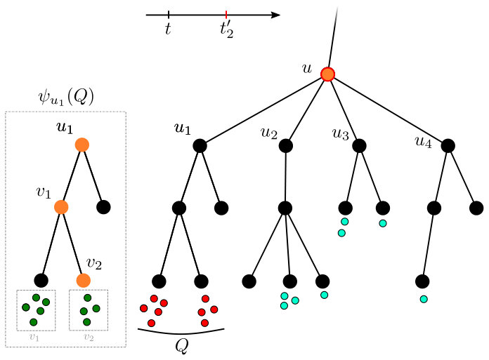 Figure 1
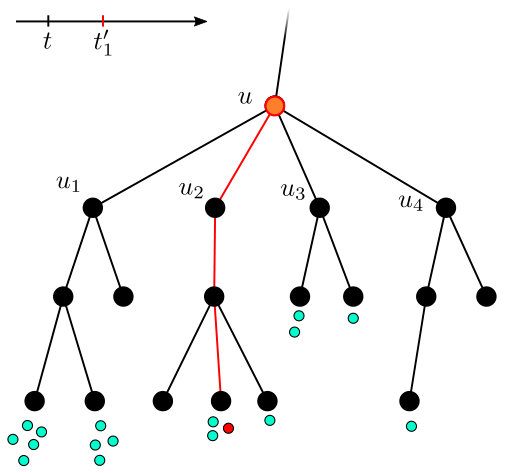 Figure 2
 Figure 3
 Figure 4
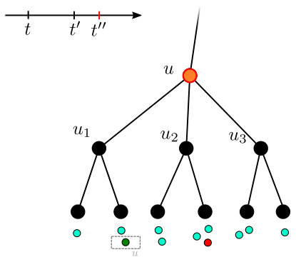 Figure 5
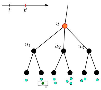 Figure 6
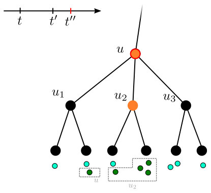 Figure 7
 Figure 8
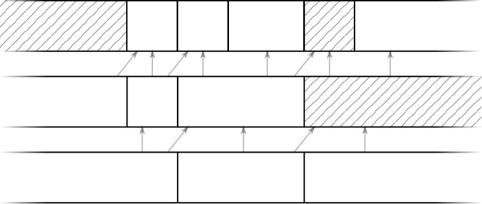 Figure 9
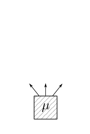 Figure 10
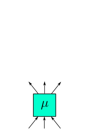 Figure 11
 Figure 12
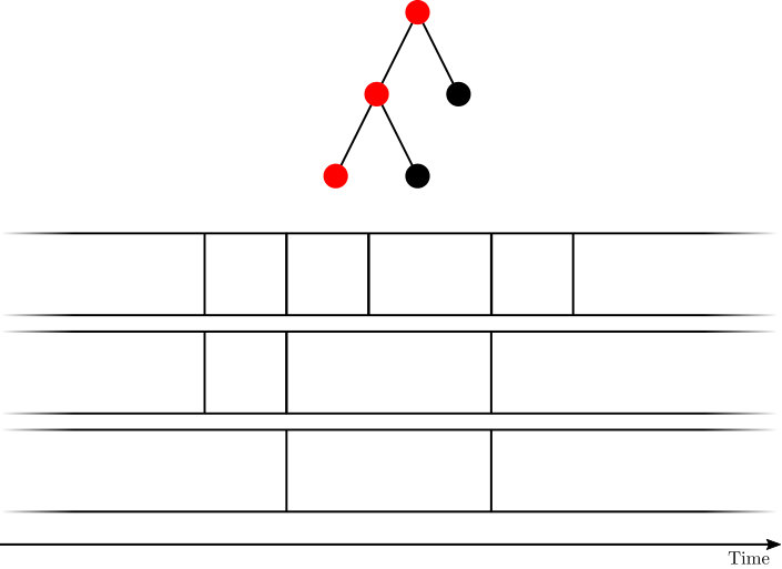 Figure 13
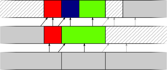 Figure 14
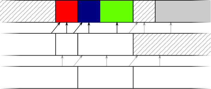 Figure 15
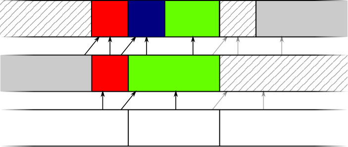 Figure 16
 Figure 17
Peer Reviews
No public reviews on file for this paper yet. If you reviewed it on a platform where reviews are public (OpenReview, ICLR, NeurIPS, ICML), you can paste yours below so the community can read it here.
Videos
No videos yet. Explain this paper in a talk, walkthrough, or lecture? Add one.
General Framework for Metric Optimization Problems with Delay or with
Deadlines
Yossi Azar
Tel Aviv University
Noam Touitou
Tel Aviv University
Abstract
In this paper, we present a framework used to construct and analyze algorithms for online optimization problems with deadlines or with delay over a metric space. Using this framework, we present algorithms for several different problems. We present an -competitive deterministic algorithm for online multilevel aggregation with delay on a tree of depth , an exponential improvement over the -competitive algorithm of Bienkowski et al. (ESA ’16). We also present an -competitive randomized algorithm for online service with delay over any general metric space of points, improving upon the -competitive algorithm by Azar et al. (STOC ’17).
In addition, we present the problem of online facility location with deadlines. In this problem, requests arrive over time in a metric space, and need to be served until their deadlines by facilities that are opened momentarily for some cost. We also consider the problem of facility location with delay, in which the deadlines are replaced with arbitrary delay functions. For those problems, we present -competitive algorithms, with the number of points in the metric space.
The algorithmic framework we present includes techniques for the design of algorithms as well as techniques for their analysis.
1 Introduction
Recently in the field of online algorithms, there has been an increasing interest in online problems involving deadlines or delay. In such problems, requests of some form arrive over time, requiring service. In problems with deadlines, each request is equipped with a deadline, by which the request must be served. In problems with delay, this hard constraint is replaced with a more general constraint. In those problems, each request is equipped with a delay function, such that an algorithm accumulates delay cost while the request remains pending. This provides an incentive for the algorithm to serve the request as soon as possible. Deadlines are a special case of delay, as deadlines can be approximated arbitrarily well by delay functions.
The mechanism of adding delay or deadlines can be used to convert a problem over a sequence into a problem over time. For example, a problem in which an arriving request must immediately be served by the algorithm can be converted into a problem with deadlines, providing more flexibility to a possible solution. This conversion often creates interesting problems over time from problems that are trivial over a sequence, as well as enables much better solutions (i.e. lower cost).
A case of special interest is the case of such problems over a metric space. A notable example, which we consider in this paper, is the online multilevel aggregation problem. In this problem, the requests arrive on the leaves of a tree. At any time, the algorithm may choose to transmit any subtree that includes the root of the tree, at a cost which is the sum of the weights of the subtree’s edges. Pending requests on any leaves contained in the transmitted subtree are served by the transmission. The general delay case of this problem was first considered by Bienkowski et al. [7], who gave a -competitive algorithm for the problem, with the depth of the tree. Buchbinder et al. [13] then showed a -competitive deterministic algorithm for the deadline case. In this paper, we improve the result of [7] for general delay exponentially.
Another notable example is the online service with delay problem, presented in [5]. In this problem, requests arrive on points in a metric space, accumulating delay while pending. There is a single server in the metric space, which can be moved from one point to another at a cost which is the distance between the two points. Moving a server to a point at which there exists a pending request serves that request. In [5], an -competitive randomized algorithm is given for the problem, where is the number of points in the metric space. This algorithm encompasses a random embedding to an hierarchical well-separated tree (HST) of depth , and an -competitive deterministic algorithm for online service with delay on HSTs. In this paper, we also improve this result to competitiveness.
In addition, we also present the problem of online facility location with deadlines. In this problem, requests arrive over time on points of a metric space, each equipped with a deadline. The algorithm can open a facility at any point of the metric space, at some fixed cost. Immediately upon opening a facility, the algorithm may connect any number of pending requests to that facility, serving these requests. Connecting a request to a facility incurs a connection cost which is the distance between the location of the request and the location of the facility. In contrast to previous considerations of online facility location, in our problem the facility is only opened momentarily, disappearing immediately after connecting the requests. We also consider the problem of online facility location with delay, in which the deadlines are replaced with arbitrary delay functions. For those problems we present -competitive algorithms, with the number of points in the metric space.
The problem of facility location is a widely researched classic problem. The modification of ephemeral facilities is highly motivated, as it describes an option of renting facilities instead of buying them. As renting shared resources is a growing trend (e.g. in cloud computing), this problem captures many practical scenarios.
Our paper presents algorithms for online facility location with deadlines, online facility location with delay, online multilevel aggregation with delay and online service with delay. These algorithms all share a common framework that we develop. The framework includes techniques for both the design of the algorithms and their analysis. We believe the flexibility and generality of this framework would enable designing and analyzing algorithms for additional problems with deadlines or with delay.
Our Results
In this paper, we present a framework used to construct and analyze online optimization problems with deadlines or with delay over a metric space. Using this framework, we present the following algorithms.
An -competitive deterministic algorithm for online multilevel aggregation with delay on a tree of depth . This is an exponential improvement over the -competitive algorithm in [7]. 2. 2.
An -competitive randomized algorithm for online service with delay over a metric space with points. This improves upon the -competitive randomized algorithm in [5]. 3. 3.
An -competitive randomized algorithm for online facility location with deadlines over a metric space with points. 4. 4.
An -competitive randomized algorithm for online facility location with delay over a metric space with points.
Our algorithms all share a common framework, which we present. The framework provides general structure to both the algorithm and its analysis.
Such an improvement for the online multilevel aggregation problem is only known for the special case of deadlines, as given in [13].
The algorithms for online facility location with deadlines and with delay can be easily extended to the case in which the cost of opening a facility is different for each point in the metric space. This changes the competitiveness of the algorithms to , where is the aspect ratio of the metric space.
Our Techniques
All of our algorithms are based on corresponding competitive algorithms for HSTs. The randomized algorithms for general metric spaces are obtained through randomized HST embedding. The -competitive deterministic algorithm for online multilevel aggregation with delay on a tree is based on decomposing the tree into a forest of HSTs. This decomposition is similar to that used in [13] for the case of deadlines.
**The framework – algorithm design. **In designing algorithms for the problems over HSTs, we use a certain framework. In an algorithm designed using the framework, there is a counter for every node (in the case of facility location) or every edge (in the case of online multilevel aggregation and service with delay). The sizes of the counters vary between the problems considered. When the counter for a tree element (either node or edge) is full, the algorithm resets the counter and explores the subtree rooted at that element.
The process of exploration serves some of the pending requests at that subtree, while simultaneously charging counters of descendant tree elements. The exploration takes place in a DFS fashion – if at any time during the exploration of an element the counter of a descendant element is full, the algorithm immediately suspends the exploration of the current element in favor of its descendant. The exploration of the original element resumes only when the exploration of the descendant is complete.
The exploration of specific element has a certain budget, used to charge counters of descendants. This budget is equal to the size of the counter of the element being explored. The algorithm adheres to the budget very strictly, spending exactly the amount specified. This is a crucial part of the framework, as exceeding the budget (or falling below budget) by even a constant factor would yield a competitiveness which is exponential in the depth of the tree.
This DFS exploration method is very different from previous algorithms, and enables us to get our improved results. The counter-based structure of our algorithms enables this DFS exploration while controlling the budget. Using the counter-based structure is, in turn, enabled by the techniques that we present in our framework’s analysis.
The framework – analysis. The analysis of the algorithms of this framework require constructing a preflow - a weighted directed graph which is similar to a flow network, but in which we allow nonnegative excesses at nodes (i.e. more incoming than outgoing). We refer to nodes of the preflow as charging nodes. We construct a source charging node, from which the output is proportional to the cost of the optimum, and then use the preflow to propagate this output throughout the preflow graph. Since the excesses are nonnegative, the sum of the excesses of any subset of charging nodes is a lower bound of the total output from the source charging node, and thus also some lower bound on the cost of the optimum. We construct the preflow in a manner that allows us to locate such a subset of high-excess charging nodes, thus providing the required lower bound.
In the preflows we construct, each tree element (node or edge) is converted to multiple charging nodes, each corresponding to an exploration of that tree element. The possible edges between charging nodes in the preflow depend on the structure of the tree and the operation of our algorithm. Of those possible edges, we describe a procedure that chooses the actual edges of the preflow. This procedure depends on the optimal solution. Though the original metric space is a tree, the multiple copies of each tree element cause the resulting preflow to be a general directed graph.
The goal of the preflow creation procedure is to propagate the optimum’s costs to some “top layer” of charging nodes. This top layer usually consists of nodes corresponding to explorations of the root tree element, though in the case of online service with delay the definition is different. The charging nodes of that top layer are then chosen to lower bound the optimum, as described.
The preflow creation procedure involves creating colors at the “top” layer of the charging nodes. These colors are then propagated, through some set of propagation rules, to nodes in lower layers. Each color corresponds to the charging node in which it originated, with the exception of two colors – the empty color, and an additional “special” color. As nodes are colored, the possible edges that contain them become actual edges of the preflow.
We now discuss the techniques used in each of the problems in this paper.
**Online facility location with deadlines. **We use our framework in constructing an algorithm for this problem over an HST. The algorithm maintains a counter on each node (other than the root node), such that each counter is of size , where is the cost of opening a facility. Whenever a counter is full, it resets and triggers an exploration of that node. Whenever the deadline of a pending request expires, the algorithm starts an exploration of the root node.
In the exploration of a node , the algorithm opens a facility at , and considers pending requests in the node’s subtree according to increasing deadline. For each request considered, it raises the counter of the child node on the path to the request by the cost of connecting that request to . If the counter of the child is full, an exploration of that child is called recursively, which would surely serve the considered request. Otherwise, the algorithm connects that request to . As per the framework, the budget of ’s exploration for raising these counters is exactly .
**Online facility location with delay. **The algorithm for this problem is an extension of the deadline case. An exploration of the root node is now triggered upon a set of requests which is critical, i.e. has accumulated large delay.
The significant difference between the delay case and the deadline case is in the exploration itself. In the deadline case, the exploration of a node spends its budget attempting to “push back” the next occurrence of a single event (i.e. the earliest deadline of a pending request in the subtree rooted at ). In the delay case, there are two events to consider. The first event is a single request with a delay large enough to justify connection to . The second event is a “coalition” of many tightly-grouped requests with small individual delay, but large overall delay. This coalition does not justify connection to , but does merit opening a facility near the coalition.
Online multilevel aggregation with delay. In our algorithm for this problem over HSTs, each edge has a counter. The size of the counter is the weight of edge. This is in contrast to our algorithms for the facility location problems, in which all counters were of the same size. We assume, without loss of generality, that there exists a single edge exiting the root node, called the root edge. As in the facility location case, an exploration of the root edge is triggered when the delay of a set of requests becomes high.
In our algorithm, exploring an edge means adding descendant edges to the transmitted subtree. The explored edge again has a budget equal to its weight. The exploration repeatedly chooses the earliest point in time in which the delay of a set of requests exceeds the cost of expanding the transmission to include these requests. It then raises the counter of the descendant edge in the direction of that request set. Note the contrast with the algorithms for facility location – the explored edge is allowed to raise the counters of its descendant edges, and not just of its immediate children.
While the analysis for our facility location problems required constructing a single preflow to get a lower bound on the cost of the optimum, the analysis for online multilevel aggregation with delay requires constructing an additional preflow to get an upper bound on the cost of the algorithm.
**Online service with delay. **Our algorithm for this problem uses the exploration method of the algorithm for online multilevel aggregation with delay. However, the tree to be explored is not the entire tree, but rather some subtree according to the location of the server. The concepts of relative trees and major edges are defined in a similar way to [5]. We also use a potential function based on the distance of the algorithm’s server from the optimum’s server. As the algorithm consists (mainly) of making calls to the multilevel aggregation exploration, the analysis divides these explorations to those for which the optimum can be charged (using similar arguments to the analysis of the multilevel aggregation algorithm), and explorations for which the costs are covered by the potential function.
Related Work
The online multilevel aggregation problem generalizes a range of studied problems, such as the TCP acknowledgment problem [14, 17, 22] and the joint replenishment problem [8, 12, 15]. For both the deadline and delay variants of online multilevel aggregation, the best known lower bounds are only constant [8]. Bienkowski et al. [7] were the first to present an algorithm for the online multilevel aggregation problem with arbitrary delay functions, which is -competitive. Buchbinder et al. [13] presented an -competitive algorithm for the special case of deadlines.
The problem of online service with delay was presented in [5], along with the -competitive randomized algorithm for a general metric space of points. The problem has also been studied over specific metric spaces, such as uniform metric and line metric, in which improved results can be achieved [5, 11].
Another metric optimization problem with delay is the problem of matching with delay [2, 19, 18, 4, 9, 10]. For this problem, arbitrary delay functions are intractable, and thus the main line of work focuses on linear delay functions.
Additional problems with delay exist other than those over a metric space. The set aggregation problem, presented in [16], is a variant of set cover with delay. The problem of bin packing with delay is presented in [3].
The classic online facility location problem, suggested by Meyerson [23], has also been studied [21, 1]. In this problem, requests arrive one after the other, and the algorithm must either connect a request to an existing facility immediately upon the request’s arrival, or open a facility at the request’s location. This problem is different from the problems of facility location with deadlines and facility location with delay presented in this paper. The main difference is that in our problems, a facility is only opened momentarily, which only allows immediate connection of pending requests. In contrast, an opened facility in the online facility location of [23] is permanent, allowing the connection of any future request to that facility.
Paper Organization
Section 2 presents the problem of online facility location with deadlines, and an -competitive randomized algorithm for the problem, as well as its analysis. Section 3 discusses the more general problem of online facility location with delay, and extending the algorithm for the deadline case in section 2 to an -competitive algorithm for the case of delay.
Section 4 presents the -competitive deterministic algorithm for online multilevel aggregation with delay. Section 5 presents the -competitive randomized algorithm for online service with delay, which relies on the algorithm for online multilevel aggregation with delay given in Section 4.
2 Online Facility Location with Deadlines
2.1 Problem and Notation
In the online facility location with deadlines problem, requests arrive on points of a metric space over time. Each request is associated with a deadline, by which it must be served. An algorithm for the problem can choose, in any point in time, to open a facility at any point in the metric space momentarily, at a cost of . Immediately upon opening the facility, the algorithm must choose the subset of pending requests (i.e. requests that have arrived but have not been served) to connect to the facility. The cost of connecting each request to the facility is the distance between the request’s location and the facility’s location. Connecting a request to a facility serves that request. Immediately after connecting the requests, the facility disappears. We allow opening a facility at the same point more than once, at different times.
Formally, we are given a metric space such that . A request is a tuple such that is a point in , the arrival time of the request is and the deadline of the request is . We assume, without loss of generality, that all deadlines are distinct. For any instance of the problem, the algorithm’s solution has two costs. The first is the buying cost (or opening cost) , where is the number of facilities opened by the algorithm. Denoting by the set of requests in the instance, and denoting by the location of the facility to which the algorithm connects request , the second cost of the algorithm is the connection cost . Wherever a single metric space is considered, we write .
The goal of the algorithm is to minimize the total cost, which is
[TABLE]
For the special case in which is a tree , and is the distance between nodes in , we denote the root of by and the weight function on the edges of the tree by . We assume, without loss of generality, that the requests only arrive on leaves of the tree.
The following definitions regarding trees are used throughout the paper.
Definition 2.1**.**
For every tree node , we use the following notations:
- •
For , we denote by the parent of in the tree.
- •
We denote by the subtree rooted at .
- •
For a set of requests , we denote by the subtree spanned by and the leaves of .
- •
We define the height of to be the depth of .
The following definition is similar to the usual definition of a -HST, except that we allow a child edge to be strictly smaller than times its parent edge.
Definition 2.2** (-HST).**
A rooted tree is a -HST if for any two edges such that is a parent edge of , we have that .
When considering the problem over a tree , we assume, without loss of generality, that for any edge . Indeed, if this is not the case, no request would be connected over , effectively yielding two disjoint instances of the problem.
In this section, we prove the following theorem.
Theorem 2.3**.**
There exists an -competitive randomized algorithm for online facility location with deadlines for any metric space of points.
2.2 Algorithm for HSTs
We present an algorithm for facility location with deadlines on a -HST of depth . We denote the root of the tree by .
We make the assumption that the total weight of any path from the root to a leaf is at most . In a -HST, the total weight of such a path is at most twice the weight of the top edge, which is at most . Thus, this assumption only costs us a constant factor of in competitiveness.
Without loss of generality, we allow the algorithm to open facilities on internal nodes of the tree. Indeed, any algorithm that opens facilities on internal nodes can be converted to an algorithm that only opens facilities on leaves in the following manner. Consider a facility opened by the original algorithm on the internal node , and denote by the set of requests connected to that facility. The modified algorithm would open the facility at instead, where , and connect the original requests. Through triangle inequality, the connection cost of the modified algorithm is at most twice larger.
**Algorithm’s description. **The algorithm for facility location with deadlines on a -HST is given in Algorithm 1. The algorithm waits until the deadline of a pending request. It then begins exploring the root node. An exploration of a node consists of considering the pending requests in by order of increasing deadline. The exploration has a budget of exactly to spend on raising counters of child nodes – it maintains that budget in the variable . When considering a request , the algorithm raises the counter of the child node , denoted in the algorithm, for the child node in the request’s direction. The counter is raised by the smallest of , the amount required to fill , and the remaining budget . If this fills the counter of , the exploration of is paused, and a new exploration of is started, in a DFS manner. We claim, in the analysis, that this exploration of connects Otherwise, the request is connected to .
The operation of the algorithm is visualized in Figure 6 of Appendix A.
2.3 Analysis
Fix any instance of online facility location with deadlines on a -HST. Let be any solution to the instance. We denote by the total buying cost of , and by the total connection cost of . Denote by the total cost of the solution of Algorithm 1 for this problem. In this subsection, we prove the following theorem.
Theorem 2.4**.**
.
To prove Theorem 2.4, we show validity of the algorithm, an upper bound for and a lower bound for .
Throughout the analysis, we denote by the number of calls to UponDeadline made by the algorithm. We also denote by the times of these calls, by increasing order.
2.3.1 Validity of the Algorithm
The following proposition and its corollary show that the algorithm is valid.
Proposition 2.5**.**
Let be a request considered in a call to . Then is served when returns.
Proof.
This is guaranteed by the condition check at the end of the main loop in Explore. ∎
Corollary 2.6**.**
Every request is served by its deadline. That is, the algorithm is valid.
Proof.
Observe that upon the deadline of a request , is called, and immediately considers . Proposition 2.5 concludes the proof. ∎
2.3.2 Upper Bounding
We now proceed to bound by proving the following lemma.
Lemma 2.7**.**
.
The proof of Lemma 2.7 is through providing an upper bound for the cumulative amount by which counters are raised in the algorithm, then bounding the cost of the algorithm by that cumulative amount.
Observation 2.8**.**
Observe any node , and consider a call to . Denote by the total amount by which increases the counters of its children nodes through calls to Invest. Then we have that . Moreover, if there exists a pending request in after the return of , then .
From the previous observation, the following observation follows.
Observation 2.9**.**
For any , is called at most once at any time .
Using the last observation, we refer to a call to at time by .
Observe the state of each counter in the algorithm over time. The counter undergoes phases, such that in the start of each phase its value is [math]. The counter increases in value during the phase until it reaches , and is then reset to [math], triggering a service and the end of the phase.
We define a virtual counter which contains the cumulative value of . That is, whenever increases, increases by the same amount, but is never reset when is reset. For the sake of analysis, we also consider a virtual counter , which is raised by whenever is called.
We define \bar{C}_{j}=\sum_{\text{node uj}}\bar{c}_{u}. Observe that .
Proposition 2.10**.**
For every , .
Proof.
Observe that the counters at depth are raised only upon a call to for a node at depth . \texttt{\textnormal{{Explore}}}(u) is only called after is raised by , and every such call raises counters at depth by at most (using Observation 2.8). ∎
Corollary 2.11**.**
.
Proof.
Observe that . Using Proposition 2.10, we have that
[TABLE]
∎
Proposition 2.12**.**
Suppose the function calls when considering request . Then at least one of the following holds:
* returns .* 2. 2.
* after the return of Invest.* 3. 3.
The condition check in Explore of whether is still pending fails.
Proof.
If does not return , and after its return, then it must be that . In this case, calls when checking the condition after the return of Invest. Request is the pending request with earliest deadline under , and thus also under . Hence, is immediately considered by , and is thus served by the end of by Proposition 2.5. ∎
Proposition 2.13**.**
**
Proof.
The costs of the algorithm (both opening and connection) are contained in calls to the function Explore (where we associate the opening costs in Open to the Explore call that invoked it). In each call to \texttt{\textnormal{{Explore}}}(u), the algorithm has a cost of in opening a facility at .
In addition, the algorithm incurs connection costs, as connects any considered request if it is still pending at the end of the loop’s iteration. From Proposition 2.12, if connects a request , then either the preceding returned , or after the return of that call to Invest.
Observe the calls to that return . For those requests, the connection cost of is exactly the return value of Invest. But the return values of Invest sum to at most the initial value of , which is . Thus, connection costs for those requests sum to at most .
As for calls to Invest after which we have that , observe that there is at most one such call, after which the loop in Explore ends. The connection cost for the request considered in this iteration is .
Overall, the connection costs in sum to at most
Thus, in each call to \texttt{\textnormal{{Explore}}}(u), the total cost of the algorithm (buying and connection) is at most . Observing that \texttt{\textnormal{{Explore}}}(u) is called only upon raising by concludes the proof. ∎
Proof of Lemma 2.7.
The lemma results directly from Proposition 2.13 and Corollary 2.11. ∎
2.3.3 Lower Bounding
We now lower bound the cost of .
Charging nodes and incurred costs.
We define a charging node to be a tuple such that , and are two subsequent times in which is called. We allow the charging nodes of the form in which and is the first time in which is called. Similarly, we allow the charging nodes in which is the last time is called, and . We denote by the set of charging nodes.
For a charging node , we define the following.
Let * *be the buying cost incurred by in , defined to be the total cost at which opened facilities in during . 2. 2.
Let be the *connection cost incurred by in , *defined to be , where is the set of requests such that , and connected to a facility outside .
Let be the total cost incurred in .
Lemma 2.14**.**
.
Proof.
We consider each action of and how it affects the incurred cost at various charging nodes.
For a facility that is opened by at node at time to participate in , we must have that . Hence, is on the branch from the root to , and thus is one of at most possible nodes. We also have that . Using Observation 2.9, we have that , and therefore can belong to at most two such intervals, for every choice of . This yields that the cost of each facility opened by is counted in ** **at most times.
As for connection costs, consider a request that connects to a facility at node . Denote by the least common ancestor of and . If incurs connection cost due to in charging node , then and . Therefore, must be on the path from to (including , and not including ). Let be the path from to . As with the buying cost, for every , may incur connection cost due to in at most charging nodes of the form for some . Therefore, denoting the total connection cost of due to connecting by , we have that
[TABLE]
Now observe that since the tree is a -HST, we have that the total weight of any path from a node to a descendant leaf is at most the weight of the node’s ancestor edge. Therefore, for every :
[TABLE]
Therefore, we have that . Hence:
[TABLE]
Since is on the path from to , we have that . Hence is at most times the connection cost of for . This concludes the lemma. ∎
Definition 2.15** (excess).**
Let be a directed multigraph, with a non-negative weight function defined on its edges. We denote by the set of edges entering node , and by the set of edges leaving . We define the *excess at a node *to be .
Note that every edge from to is counted in and with opposite signs. The following observation follows.
Observation 2.16**.**
For any and weights , we have .
Definition 2.17**.**
For a graph and non-negative weights , We say that is a *preflow *if for every node we have that . We call the *source node *of the preflow.
Observation 2.16 yields that for every preflow . We write .
Proposition 2.18**.**
For a directed graph, for weights such that is a preflow, and for every , we have .
Proof.
Observation 2.16 and the definition of a preflow, we get . ∎
We now construct a preflow to lower bound . The graph underlying the preflow has the set of nodes , where is the set of charging nodes and is a source node.
Consider a charging node . We have that corresponds to a phase of the counter , since was empty at and was filled and emptied again until time .
Definition 2.19** (Investing).**
Observe two charging nodes and . We say that *invested in *if the function call increased by , through calls to Invest, during the phase of between and .
Definition 2.20** ( and ).**
For every function call for some and time , we denote by the earliest deadline of a pending request in immediately after the return of (if there are no pending requests in , we write ).
In addition, for a charging node with , we write .
Possible edges.
We describe the set of possible edges in from nodes in to other nodes in , denoted by , and the weight function . The final set of edges added to by Procedure 3 from the nodes of to themselves is a subset of . The set contains an edge from any charging node to any charging node if invested in . We set the weight to be the amount that invested in .
In the analysis of the preflow resulting from this procedure, we refer to the values of the variables used in the procedure in their final state.
Proposition 2.21**.**
For every charging node , we have that .
Proof.
Observe that is a subset of . In , the sum of over edges outgoing from is exactly the amount invested in other charging nodes, which is at most . ∎
Corollary 2.22**.**
For a charging node in which we have .
Proposition 2.23**.**
Let be such that for some charging node . Then did not open a facility in during .
Proof.
Since , we have that did not open a facility in during .
The proof is by induction on the depth of . If , then it must be that , completing the proof. Otherwise, observe the node from which inherited its color. By the induction hypothesis, did not open a facility in during . Since there exists an edge from to , we must have that , which completes the proof. ∎
Lemma 2.24**.**
* is a preflow. That is, for every charging node we have .*
Proof.
We observe the following cases according to the final values of the variables in the graph construction procedure.
Case 1: \texttt{\texttt{Color}}[\mu]=\texttt{Special}. In this case, opened a facility in during , implying that . In the initialization of Procedure 3, an edge from to with is created, and thus Corollary 2.22 implies that .
Case 2: for some charging node . In this case, incoming edges to were added, with a total weight which is the total amount invested by . Since was set by SetColor, we must have that and that . Using Observation 2.8, we have that raised counters by a total of exactly . Corollary 2.22 therefore proves the lemma for this case.
Case 3: . Observe any edge , incoming to some node . It must be that , for some charging node . Note that invested in , and thus . Combining Proposition 2.23 for and the fact that , we have that did not open a facility in during .
We therefore have that for every request such that and , must connect to some facility at a node . If it also holds that , then incurs a connection cost of in on connecting . We proceed to find such requests .
Now observe that invested in . Thus, there exists a set of requests that are considered in such that and for every . Since the requests of are considered in , we have that for every . Since , we have that , and thus .
Observe any . It holds that , since is considered in . Now, observe that even though . Hence, either or . If , then . Otherwise, and . Since , it must be that was not pending immediately after the return of . However, considered when raising toward . Thus, was released after .
Overall, for every we have that and . Thus, incurs a connection cost of at least in the charging node due to , which is at least .
Now, if for every distinct we have that , then the connection cost incurs in is at least . Indeed, observe that and enter two distinct charging nodes and . Lemma 2.9 implies that . It is enough to observe that for , each request is pending before and is served after .
Overall, we have that . In the initialization of Procedure 3, an edge from to with is created, and thus as required. This concludes the proof of the current case, and the lemma. ∎
Lemma 2.25**.**
For each and charging node , we have .
Proof.
Observe that . It remains to see that .
If , it holds that identically to Cases 1 and 2 in Lemma 2.24.
Otherwise, we must have that returned None. Thus, it must be that either or . We claim that either of these cases contradicts . Indeed, observe that is called upon a deadline of a request . If , it holds that . If , it must be that as well. Overall, , and thus must open a facility in that interval, in contradiction. ∎
Lemma 2.26**.**
**
Proof.
Lemma 2.24 yields that is a valid preflow. For , let . Using Lemma 2.25 and Proposition 2.18, we have that
[TABLE]
Now observe that , and that . Using Lemma 2.14, we obtain
[TABLE]
as required. ∎
Proof of Theorem 2.4.
Combining Lemmas 2.7 and 2.26, we have that
[TABLE]
∎
Remark 2.27*.*
Our algorithm and its analysis also work in the case that the cost of opening a facility is different between nodes in the tree, as long as the cost of opening a facility at a node is at least the cost of opening a facility at its parent node. If this is not the case, observe that the analysis of Case 1 of Lemma 2.24 would no longer hold.
2.4 From HST to General Metric Space
In this subsection, we show how the deterministic Algorithm 1 for -HSTs yields a randomized -competitive algorithm for facility location with deadlines on a general metric space with points, thus proving Theorem 2.3. To do this, we consider a standard probabilistic embedding of a metric space to an HST.
Theorem 2.28**.**
For any metric space such that , there exists a distribution over -HSTs of depth such that are the leaves of the HST, such that the expected distortion is . That is, for every we have that
[TABLE]
where is the distance in the tree .
Theorem 2.28 is a direct result of composing the embeddings of Fakcharoenphol et al. [20] and Bansal et al. [6].
We observe the following randomized algorithm for facility location with delay on a general metric space:
Embed the metric space to a -HST according to the distribution in Theorem 2.28. 2. 2.
Run Algorithm 1 on the resulting -HST.
Proof of Theorem 2.3.
We show that the randomized algorithm described above is indeed -competitive. Fix any instance of facility location with deadlines. We denote by the cost of the algorithm on the instance with regard to distances on the chosen -HST . Since , we have that , where is the actual cost incurred by the algorithm on this instance.
From Theorem 2.4, we know that for any solution for the instance on , it holds that , where is the depth of (and thus ).
Now, denote by the optimal solution for the instance over . Observe that for every in the support of , yields a solution by opening facilities at the same locations, at the same times, and connecting the same requests. It holds that , and that .
Combining the above facts, we have that
[TABLE]
proving the theorem. ∎
The reasoning behind the main theorem of this subsection is that the connection cost is distorted upon HST embedding, while the buying cost is not. Thus, the HST algorithm is allowed to lose a larger factor over () compared to the factor it loses over (). This property is used to analyze the other problems considered in this paper in a similar manner.
Remark 2.29*.*
For the case of different costs for opening facilities at different points in the metric space, we obtain a -competitive randomized algorithm, with the aspect ratio of the metric space, in the following manner. We use the embedding of Fakcharoenphol et al. [20] without composing it with the embedidng of [6]. This yields a 2-HST (rather than a -HST), which has a depth of , with the aspect ratio of the original metric space. This tree has an distortion of .
In this -HST, for each node , the distances between and the leaves in are equal. Thus, we can allow the algorithm to open a facility at , at a cost which is the minimal cost of opening a facility at a leaf in , at a loss of a factor of in connection cost. The resulting tree has non-decreasing opening costs from the root to any leaf, and is (in particular) a -HST of depth . Thus, using the algorithm for -HSTs and Remark 2.27, and applying the distortion of to the connection cost as in the proof of Theorem 3.1, we obtain the -competitive algorithm.
3 Facility Location with Delay
3.1 Problem and Notation
We now describe the facility location with delay problem. The problem is an extension of the facility location with deadlines problem, in which the deadline for each request is replaced with an arbitrary delay function associated with that request. Each delay function is required to be continuous and monotonically non-decreasing. This is indeed an extension of the deadline problem, as a deadline can be described as a step function, which goes from [math] to infinity at the time of the deadline. Such a step function can be approximated arbitrarily well by a continuous delay function.
A feasible solution for a facility location with delay instance consists of opening facilities and connecting each request to some facility, as in the deadline case. In addition to the opening costs and connection costs incurred, the solution also pays for each request connected at time . Overall, for an instance of the problem with requests , the algorithm incurs the delay cost , where is the time in which is served by the algorithm. Thus, the algorithm’s goal is to minimize the total cost
[TABLE]
Without loss of generality, we assume that . Indeed, if this is not the case, observe that any solution (including the optimal one) must pay this initial amount of in delay for that request, which only reduces the competitive ratio of any online algorithm.
In this section, we prove the following theorem.
Theorem 3.1**.**
There exists an -competitive randomized algorithm for facility location with delay for a general metric space of size .
3.2 Algorithm for HSTs
In this subsection, we present a deterministic algorithm for facility location with delay on a -HST. This algorithm yields a randomized -competitive algorithm for general metric spaces, in a similar way to the deadline case.
We require the following definitions.
Definition 3.2** (Solution).**
Let be a set of requests. For , and a function we say that is a *solution for *, with a cost . If for some node , we write that is a solution for under .
Definition 3.3** (Ancestor-closed solution).**
Let be a set of requests, and let be a solution for under a node . We say that is an *ancestor-closed solution for under *if for every such that we have that .
If , we simply write that is an ancestor-closed solution for .
Definition 3.4** ( and ).**
We define to be the cost of the minimal-cost ancestor-closed solution for . Similarly, we define to be the cost of the minimal-cost ancestor-closed solution for under .
Definition 3.5** (Critical request set).**
We say that a set of pending requests at time is *critical *if .
**Algorithm’s description. **Our algorithm is given in Algorithm 5. The algorithm calls UponCritical whenever a set of pending requests becomes critical. It uses the Open and Invest functions from Algorithm 1, but redefines the Explore function. The function call now forwards time until the first occurrence of one of two events.
The first event is a pending request in , the delay of which exceeds the cost of connecting it to . Handling this event is similar to handling the event considered in Algorithm 1 – we attempt to raise the counter of the child node in ’s direction by . If this fills the counter of , this triggers an immediate call to . However, in contrast to the deadline case, calling is not guaranteed to connect the request . For this reason, must invest the remainder of (or until ) in ’s counter before connecting to .
The second event is not analogous to the deadline case. In this event, for a child of and a “coalition” of pending requests in , we have that the delay of exceeds . In this case, the algorithm invests in until either it is out of budget () or ’s counter is full ). It is important to note that in contrast to the first event, the fact that considered does not provide any guarantees for connecting the requests of .
Algorithm 5 changes so that time is forwarded until one of two events happens, rather than the single event in Algorithm 1 (i.e. expired deadline). These two events are shown in Figure 4.
3.3 Analysis
Fix any instance of facility location with delay on a -HST.
Theorem 3.6**.**
.
Observe that the connection cost is distorted by the embedding, while the buying and delay costs are not. Thus, using an identical argument to the proof of Theorem 2.3 of the deadline problem, Theorem 3.6 implies Theorem 3.1.
We devote this subsection to prove Theorem 3.6.
3.3.1 Upper Bounding
To upper bound the cost of the algorithm, we show the following Lemma.
Lemma 3.7**.**
**
Proposition 3.8**.**
**
Proof.
The algorithm explicitly maintains that for every set of pending requests at any time we have that . Now, consider that since the delay of a pending request goes to infinity, the algorithm ultimately serves every request. Consider a specific service made by the algorithm, described by a solution to some set of requests , and note that is an ancestor-closed solution to . Thus, its total cost is at least , completing the proof. ∎
Lemma 3.9**.**
.
Proving Lemma 3.9 is very similar to proving Lemma 2.7 of the deadline case. Defining cumulative counters as in the deadline case, we can prove Corollary 2.11 holds in the delay case using an identical proof. It remains to show and prove analogues to Propositions 2.12 and 2.13.
Note that the connection costs in only occur during iterations of the main loop in which the main if condition is entered.
Proposition 3.10** (analogue of Proposition 2.12 ).**
*Suppose the function enters the main **if *condition in an iteration, and let be the pending request under consideration. Then at least one of the following holds:
The sum of return values of calls to Invest in that iteration is . 2. 2.
* at the end of the iteration.* 3. 3.
* is no longer pending after the first call to Invest.*
Proof.
Consider the state after the return of the first call to Invest. Either Invest returned , or , or . In the first two cases, we are done. In the third case, then calls . If is connected during , we are done. Otherwise, enters the nested **if **condition upon observing that is still pending.
Denote by the return value of the first call to Invest, and consider the return value of the second call to Invest made in the nested if. If the return value is , we are done. Otherwise, consider that before the call to Invest, and since it must thus be that after the return of the second call to Invest. This concludes the proof. ∎
Proposition 3.11** (analogue of Proposition 2.13).**
**
Proof.
The costs of the algorithm (both opening and connection) are again contained in calls to Explore, as in the proof of Proposition 2.13. Each call to has an opening cost of .
As for connection costs, note that they only occur in iterations of the main loop in in which the main **if **condition is entered, and not in the else condition. In each iteration in which the main if condition is entered, a request is considered, which may be connected to at cost . Through Proposition 3.10, in each such iteration either the return values of calls to Invest sum to (and thus decreases by ), at the end of the iteration (in which case this is the last iteration), or does not connect .
Since can decrease by at most , the connection cost of the algorithm is bounded by for the last request considered, which is at most .
Noting that the total cost of is at most , and that is raised by before calling yields the proposition. ∎
Proof of Lemma 3.9.
Results directly from Proposition 3.11 and Corollary 2.11 (which holds for the delay case as well). ∎
Proof of Lemma 3.7.
The lemma results directly from Proposition 3.8 and Lemma 3.9. ∎
3.3.2 Lower Bounding
To lower bound the cost of the optimum, we prove the following lemma, which is analogous to Lemma 2.26 of the deadline case.
Lemma 3.12**.**
.
Charging nodes and incurred costs.
We again use charging nodes, defined as in the deadline case. However, the charging nodes for the delay case use half-closed intervals instead of the closed intervals of the deadline case. The reason for this is that we do not have the guarantee that only one call to UponCritical is made at a given time, so that using closed intervals would break the analogue of Lemma 2.14 for our case.
Let be the set of charging nodes. The definitions of (buying costs) and (connection costs) are identical to the definition in the deadline case. For the delay case, we also define incurring *delay *costs,
Definition 3.13** ().**
Let be a charging node. Let be the *delay cost incurred by on *, defined to be the total delay cost incurred by on requests in released in .
We write .
We use Procedure 3 to create the preflow. However, we give a different definition to than in the deadline case. The definition follows.
Definition 3.14** ( and ).**
For every function call for some and time , let be the set of requests pending in immediately after the return of . We define to be the first time in which one of the following conditions occurs:
There is a request such that . 2. 2.
There exists a set of requests such that , for some a child of , and also .
Like in the deadline case, we write where .
Lemma 3.15**.**
.
Proof.
can be charged to and can be charged to as in Lemma 2.14 (since the intervals are not closed, this improves by a factor of ). It remains to charge to . To do so, observe that the delay incurred by on a request can only be counted in charging nodes with intervals containing , and defined by a node which is an ancestor of . There are at most such nodes. ∎
Observation 3.16**.**
Let be a minimal-cost ancestor-closed solution for under . Then it holds for every that the least ancestor of in .
Observation 3.17**.**
Let be a minimal-cost ancestor-closed solution for under . Let be a descendant of . Observing the set , we have that is a minimal-cost ancestor-closed solution for under .
Proposition 3.18** (Decomposition of minimum-cost ancestor-closed solutions).**
Let be a minimum-cost ancestor-closed solution for under , and let be the children of in . Define , and define . Then
[TABLE]
Proof.
For every , Observation 3.16 implies that the requests of only connect to facilities in . The opening costs of , plus the connection costs of , are exactly according to Observation 3.17, for a total of .
In addition, opening the facility at costs . Observation 3.16 implies that the requests of are connected to the facility at , at a total cost of . This finishes the proof of the proposition. ∎
Lemma 3.19**.**
* for every . That is, the preflow defined in Procedure 3 is valid.*
Proof.
We observe the following cases for .
Case 1: . This case is identical to Case 1 in Lemma 2.24.
Case 2: for a charging node . Again, this case is similar to Case 2 in Lemma 2.24.
From now on, assume we are not in the previous two cases, and thus . Every outgoing edge from to some charging node is created from investing in , which means that raised the counter towards .
**Case 3: **For every such , we have that raised towards only through calls to Invest inside the main **if **condition of Explore, and not through the main **else **condition. In this case, we show that , proving the lemma for this case. The proof is almost identical to the proof of Case 3 of Lemma 2.24, in which we showed for the deadline case that . The argument for the deadline case consisted of finding a set of requests which the optimum had to connect, all released in . The difference between our delay case and the deadline case is that might choose not to connect some of those requests, in which case it must incur a delay cost which is at least its connection cost.
**Case 4: **There exists an outgoing edge from to a charging node , such that raised towards through calls to Invest inside the main **else **condition of Explore. Let . Observing that Proposition 2.23 holds for the delay problem as well, and using , we have that did not open a facility in during .
Since raised towards inside the main **else **condition, there was a set of requests pending at such that there exists a time in which . In addition, the main **else **condition is only reached if . Thus, for every request we have that .
Observe that every is pending at , and thus released prior to . Showing that , together with the fact that did not open a server in during , would yield that either:
- •
connected to a facility outside at a cost of at least , which is at least , or
- •
did not connect until time , in which case it paid a delay cost of .
In either case, paid at least in delay and connection costs on . Since we have that , we have that incurred a cost of in due to . It remains to find a set of such requests such that for every , and such that .
**Claim: **there exists a set of requests such that for every , and such that .
Now, since , we have that either or . If , then for every . Since , choosing completes the proof of the claim.
Otherwise, and . Let be the minimal-cost ancestor-closed solution for under . Defining , and for every as in Proposition 3.18, we have that
[TABLE]
Now, denote by the subset of that was pending immediately after . We make the following observations.
For every , we have that . Otherwise, would become critical before . But since , we must have that . Thus, . 2. 2.
Writing , we observe that since , we have that
Overall, we get that
[TABLE]
Thus, we have that
[TABLE]
Observing that for each yields the claim, and thus the lemma. ∎
Lemma 3.20**.**
For every , the charging node has .
Proof.
Observe that . It remains to see that .
If , this holds similarly to Lemma 2.25.
Otherwise, assume that . Since , did not open a facility in . We find a set of requests released in on which incurs at least delay. The argument that follows is similar to that of Case 4 of Lemma 3.19, the structure of which we repeat for clarity.
We must have that either or . Denote by the set of requests that triggered the service at . We have that . Observe that for every . If , then for every , and since the proof is complete.
Otherwise, . Denoting by the minimum-cost ancestor-closed solution for , we define , and for every as in Proposition 3.18. Proposition 3.18 yields
[TABLE]
Define to be the subset of alive immediately after the return of . Using , and choosing , we use an identical argument to Case 4 of Lemma 3.19 to show that
[TABLE]
Choosing completes the proof of lemma, identically to Case 4 of Lemma 3.19. ∎
We can now prove Lemma 3.12.
of Lemma 3.12.
Lemma 3.19 yields that is a valid preflow. For , let . Using Lemma 3.20 and Proposition 2.18, we have that
[TABLE]
Now observe that , and that . Using Lemma 3.15, we obtain
[TABLE]
as required. ∎
Proof of Theorem 3.6.
Using Lemmas 3.7 and 3.12 completes the proof. ∎
4 Online Multilevel Aggregation with Delay
4.1 Problem and Notation
In the online multilevel aggregation with delay problem, requests arrive on the leaves of a rooted tree over time. Each such request accumulates delay until served. At any point in time, an algorithm for this problem may choose to transmit a subtree which contains the root, at a cost which is the weight of that subtree. Any pending requests on a leaf in the transmitted subtree are served by the transmission.
Formally, as in the facility location with delay problem, a request is a tuple where the leaf of the request is , the arrival time of the request is and is the request’s delay function. The function is again required to be non-decreasing and continuous.
We observe online multilevel aggregation with delay on a -HST. We assume, without loss of generality, that only a single edge exits the root node, called the root edge. Otherwise, we operate on each edge that exits the root node separately, as there is no interaction between the subtrees rooted at those edges. We denote the tree by , and its root edge by .
For a request , and a set of edges we write that if the leaf edge on which is released is in . In accordance, we write if for every . For a set of pending requests at time , we denote by the total delay incurred by the requests of until time . We denote by the weight of an edge, and by the total weight of a set of edges.
We assume that each request would gather infinite delay if it remains pending forever.
The following notations are similar to those for facility location, but refer to edges instead of nodes.
Definition 4.1** (Similar to Definition 2.1).**
For every tree edge , we use the following notations:
- •
For , we denote by the parent edge of in the tree.
- •
We denote by the subtree rooted at .
- •
For a set of requests , we denote by the subtree spanned by and the leaves of . We denote .
- •
We define the height of , denoted , to be the depth of .
In this section, we prove the following theorem.
Theorem 4.2**.**
There exists a -competitive deterministic algorithm for online multilevel aggregation with delay on any tree of depth .
4.2 Algorithm for HSTs
We now present an algorithm for the online multilevel aggregation with delay problem over a -HST of depth .
Definition 4.3** (saturation and critical sets).**
For any edge , we say that a set of pending requests *saturates * if . We say that a set of pending requests is critical at time if saturates the root edge .
Upon a set of critical requests, the algorithm starts a service. In every service, the algorithm maintains a tree , which it expands and ultimately transmits.
Definition 4.4** (live cut).**
At any time during the construction of , we define the *live cut under *to be the set of edges .
**Algorithm’s description. **The algorithm is given in Algorithm 6. When a set of requests is critical, a call is made to UponCritical, which resets the tree to transmit , calls to expand , then transmits .
The exploration of an edge adds to . It then considers the live cut underneath , which is the set of potential candidates for expanding . The exploration forwards time until a set of pending requests saturates for an edge in the the live cut. It then invests in raising the counter of , until either the counter is full (which triggers immediately) or is out of budget. The counter of , as well as the budget of , is equal to .
Note that the live cut under can change significantly after every iteration of the loop in , as making a recursive call to can add many additional edges to .
4.3 Analysis
Fix any instance of online multilevel aggregation with delay, and observe the behavior of Algorithm 6 for that instance. We denote by the algorithm’s total cost. We also define to be the algorithm’s buying cost, and to be the algorithm’s delay cost, such that . We similarly define and for the optimal solution for the instance.
In this subsection, we prove the following theorem.
Theorem 4.5**.**
**
In the following analysis, we denote by the number of times that the algorithm transmits a tree. We also denote the times of the transmissions by in increasing order.
4.3.1 Upper Bounding
We upper bound the cost of the algorithm by proving the following lemma.
Lemma 4.6**.**
**
The main technique used in proving Lemma 4.6 is constructing a preflow to provide an upper bound for . Bounding by then yields the lemma.
Observation 4.7**.**
Every call to serves at least one pending request.
Proposition 4.8**.**
Every request is eventually served.
Proof.
Consider a request . As assumed in the model, the delay of goes to infinity as remains pending. But at some point, the delay of would exceed , making critical, and triggering calls to until is served. Each such call serves at least one pending request due to Observation 4.7, and thus will eventually be served. ∎
The following observation follows from the fact that a tree is transmitted whenever a set of requests becomes critical.
Observation 4.9**.**
At any time during the algorithm, and for any set of requests pending at , it holds that .
Lemma 4.10**.**
.
Proof.
Denote by the set of all requests released in the instance. Through Proposition 4.8, we can partition into the sets of requests , for , such that is served in the ’th service. Denote by the tree bought by the algorithm in the ’th service, and denote by the total delay incurred by the algorithm on the requests of . To prove the lemma, it is enough to show that for every .
Now, observe that since all of are served in . Therefore, . Since transmitting serves , we have that . Using Observation 4.9, we have that as required. ∎
It remains to bound .
Let be the set of calls to Explore made by the algorithm. Observe that in the algorithm, whenever an edge is bought, a call to Explore() is made immediately afterwards. Therefore, we have that .
In addition, immediately prior to calling Explore() the counter is zeroed. We say that *invested * in if raised by , such that the next zeroing of triggers .
We now construct a graph and a weight function , such that is a preflow. We construct and in the following way:
For every , and for every root function call , add to an edge from to , and set . 2. 2.
For every function call , and for each function call that invested some amount in , we add to an edge from to , and set .
Lemma 4.11**.**
For every we have that , implying that is a valid preflow.
Proof.
We first claim that . If , this is true since there exists an edge from to such that .
Otherwise, observe that the total amount invested in is exactly , and thus .
Now, observe that invests at most in counters for edges of height at most , and thus . Combining this with the previous claim, we get as required. ∎
We can now prove Lemma 4.6.
of Lemma 4.6.
Observe the preflow . Note that
[TABLE]
Using Lemmas 4.11 and 2.18, we have
[TABLE]
Using Lemma 4.10, we get that as required. ∎
4.3.2 Lower Bounding
The following lemma provides a lower bound on the cost of the optimum.
Lemma 4.12**.**
.
Charging nodes and incurred costs.
We now define charging nodes for the analysis of our algorithm. The charging nodes are tuples of the form , such that and are two subsequent times in which the edge is bought. As in the facility location case, we allow and .
For a charging node we say that:
- •
incurs a *buying cost *of in if bought the edge during . We denote the buying cost that incurs in by .
- •
incurs a *delay cost *in equal to the delay incurred by on the set of requests . We denote the delay cost that incurs in by .
We denote the total cost that incurs in by .
Denote by the set of all charging nodes. To prove Lemma 4.12, we show a preflow on the set of vertices , where is the source node.
The following definition of charging node investment is very similar to the definition for the facility location case.
Definition 4.13** (Investing).**
For two charging nodes and , such that is an ancestor of , we say that *invested in *if raised the counter by , through calls to Invest, during the counter phase of between and .
Definition 4.14** ( and ).**
For every function call for some edge and time , let be the set of requests pending in immediately after the return of . We define to be the first time such that there exists such that .
For a charging node such that , we write .
Possible edges.
We describe the set of possible edges in from nodes in to other nodes in , denoted by , and the weight function . The final set of edges added to by Procedure 8 from the nodes of to themselves is a subset of . The set contains an edge from any charging node to any charging node if invested in . We set the weight to be the amount that invested in .
We can now construct the preflow required for the analysis using Procedure 8. This procedure is very similar to Procedure 3, used for analysis of our algorithms for facility location. It uses the function SetColor as defined in Procedure 3.
The procedure for the construction is given in Procedure 8 very similar to that given in Procedure 3.
Definition 4.15** (Cut).**
We say that a set of edges is a *cut *if no edge in is an ancestor of another edge in .
It is easy to verify that any live cut is a cut.
Proposition 4.16**.**
Let be an edge, and let be a cut in that does not include . Let be a set of pending requests and be a time such that . Then there exists an and a subset such that and .
Proof.
Partition into disjoint sets for every , according to the subtree in which the requests are. Now, observe that . We thus have that
[TABLE]
and thus there exists such that , as required. ∎
Proposition 4.17**.**
Observe the function call , and let be the set of times chosen as in . Then for every we have that .
Proof.
Fix some point during the execution of . Denote by the set of pending requests in , and let be the first time such that there exists for which . Observe the next time chosen as in . Observe that the subtrees rooted in edges of the current live cut contain all of . Thus, using Proposition 4.16, we obtain that .
Since during requests are being served but do not arrive, we have that only increases during . Since the final value of is , for every we have as required. ∎
Proposition 4.18**.**
For every charging node , it holds that .
Proof.
Observe that an outgoing edge from only goes to a node that invested in , and is labeled where is the amount that invested in . These amount sum to at most , since the counter can only reach before it is zeroed and is bought (thus ending the counter phase ). ∎
Corollary 4.19**.**
Every charging node such that has that .
The following observation results from the condition checks in SetColor.
Observation 4.20**.**
For any node such that for some charging node , we have that , and also .
The following Proposition is analogous to Proposition 2.23, and its proof is identical.
Proposition 4.21**.**
Let such that for some charging node . Then did not transmit during .
Lemma 4.22**.**
The preflow defined by Procedure 8 is valid.
Proof.
We need to show that for every .
We consider the following cases:
Case 1: . In this case, we have that . Observe that an edge from to is created with , and thus from Corollary 4.19 we have that .
Case 2: , for some charging node . Using Observation 4.20, observe that and , and thus the call has raised counters by exactly , and thus has invested a total of in other charging nodes. Thus, in . Observe that SetColor added the edges of to , and thus . Using Corollary 4.19, we have that .
Case 3: . If there are no outgoing edges from , then clearly and we are done. Otherwise, there exists an outgoing edge to some node with , for some charging node . Denote , and observe that since invested in , we must have that . Using Proposition 4.21, and the fact that , we have that did not transmit during .
**Claim – **There exists a set of requests such that such that .
Proof of Claim.
Since , it must be that and . Since invested in , we have that at some point during , was in the live cut under , and the algorithm detected a set of pending requests such that for some time . From Proposition 4.17, we have that . Note also that since is pending at , we have that . for every .
Now observe that since , , and there exists an edge from to , we must have that was called. Since , it must be that either or .
If , then for every . Combining this with , we have that for every . We also have that , by ’s definition. Thus choosing proves the claim for this case.
Otherwise, we have that and . We denote by the subset of requests pending immediately after the return of . By the definition of , and since , we have that . Thus,
[TABLE]
Denote . The requests of were not pending immediately during , and therefore for any . As seen before, for every we have that , and thus for any we have . therefore proves the claim. ∎
We now use the claim. As shown before, did not buy during , and has therefore did not serve any request from until time . Therefore, incurs a delay cost of at on the requests of , and thus . Observe that an edge from to is created with , and thus Corollary 4.19 implies that . This concludes the proof of Lemma 4.22. ∎
Lemma 4.23**.**
For every , the charging node has that .
Proof.
We denote . Observe that no other nodes invest in , and thus . It remains to show that .
If , then identically to Cases 1 and 2 of Lemma 4.22, we have that . This completes the proof for these cases.
If , then we have a very similar proof to case 3 of Lemma 4.22. Observe the pending requests that became critical at , triggering the service. Clearly, for every . Observe that was called, yet . Thus, it must be that either or . To complete the proof, we need the following claim.
**Claim – **there exists a set of requests such that for every , and .
Proof of Claim.
Observe the two cases of the claim. If , then for every . Together with the fact that , choosing proves the claim.
Otherwise, and . In this case, denote by the requests of pending immediately after and observe, as in Case 3 of Lemma 4.22, that . Thus, we have that . Observe that for every , and thus for every . Thus choosing yields the claim. ∎
Now, observe that and thus did not transmit during . Using the claim, incurred delay cost of at least on due to . Thus , and thus , completing the proof of the lemma. ∎
Proposition 4.24**.**
**
Proof.
Observe that , and that for every to a node we have that . Therefore, .
Observe that for buying an edge at time , incurs buying cost only at the unique charging node such that .
In addition, when incurs delay for a request released on leaf edge , it incurs delay cost in at most charging nodes, of the form such that and is an ancestor of .
Thus, , proving the proposition. ∎
We can now prove Lemma 4.12.
Proof (of Lemma 4.12).
Observe the set of charging nodes . Using Lemma 4.23, we have that .
We now use Propositions 2.18 and 4.24 to obtain
[TABLE]
proving the lemma. ∎
We now prove the main theorem for this subsection.
Proof of Theorem 4.5.
The theorem results immediately from Lemmas 4.6 and 4.12. ∎
4.4 From HSTs to General Trees
In this subsection, we show how to extend our result for multilevel aggregation on -HSTs to general trees, thus proving Theorem 4.2. To do so, we use a similar method to that used in [13] to form a virtual forest of -HSTs, based on the edges of the original tree.
The decomposition.
Let be the tree, with general weights, rooted at root edge . We create a forest, the edges of which are the edges of .
Definition 4.25** (parenthood in virtual -HST).**
For every edge , we define , the *virtual parent *of , to be the least ancestor of in such that . If there is no such , then is *the root edge *of a virtual tree in the forest.
We define the forest according to the function . Observe that each connected component is indeed a tree, and specifically a -HST. Denote by the virtual trees formed from , and denote by the root edge of
Let be an instance of online multilevel aggregation with delay. We partition the requests of to , such that a request belongs to if the leaf edge .
We denote by the optimal solution for the multilevel aggregation instance in the virtual tree . Using an identical argument to Observation 4.2 in [13], we have the following observation.
Observation 4.26**.**
**
Definition 4.27**.**
Let . We define to be the set of edges in on the path from to (including , not including ). If , then let be all the edges from to , including .
Definition 4.28**.**
Let be some transmittable subtree in for any . We define to be the *concretization *of .
The algorithm.
We now describe the algorithm for online multilevel aggregation with delay on a general tree. The algorithm is:
Run Algorithm 6 for each of separately. 2. 2.
Whenever the instance of Algorithm 6 for transmits the virtual subtree , transmit its concretization .
Observe that any transmission made by the main algorithm indeed serves the same requests as the original, virtual transmission. We denote by the virtual cost of the -HST algorithm for – that is, the delay of the requests of plus the sum of the costs of virtual transmissions triggered by the -HST algorithm for .
We denote by for the number of transmissions caused by the algorithm for . The following lemma is a restatement of Lemma 4.12.
Lemma 4.29**.**
**
It remains to bound the cost of the algorithm.
Proposition 4.30**.**
**
Proof.
Observe that and that . Thus, we have that
[TABLE]
where the second inequality is from Lemma 4.10. ∎
We denote by where is the ’th transmission made by the algorithm. Observe that .
The following lemma bounds the cost of the algorithm, and provides the final component for Theorem 4.2.
Lemma 4.31**.**
For every , we have that .
Fix . We denote by for the ’th virtual transmission made by the -algorithm. For , we denote by the time of ’s transmission.
To prove Lemma 4.31, we construct a preflow, in a similar manner to the proof of Lemma 4.6. However, in this case we also have nodes that correspond to edges that for which Explore is not called.
We now describe the construction of the graph , and the weight function , such that is a preflow. Each vertex in is of the form where . To describe the edge set , we require the following definition.
Definition 4.32** (-route).**
Let , be two edges such that is an ancestor of , and . Denote by the path from to in . We define an -route from to to be the set of the following charging node edges.
An edge from to with . 2. 2.
For each , an edge from to with .
We also define an -route from to in a similar manner. Let the path from the root of to . The edges of this -route are:
An edge from to with . 2. 2.
For each , and edge from to with .
We can now describe . The edges of are constructed in the following way:
For each , add to the edges of a -route from to . 2. 2.
For two charging nodes , such that , is an ancestor of and invested in , add to the edges of an -route from to .
Observation 4.33**.**
For every two edges , such that it holds that .
Lemma 4.34**.**
For every charging node it holds that .
Proof.
Observe that -routes do not
It must be that . Hence, there exists an edge such that . Since , then we are in one of the following cases.
Case 1: , and thus . It can be shown that , and that , similarly to the proof of Lemma 4.11.
Case 2: and . Thus, . Observe that since , adding any -route cannot decrease . Indeed, adding an -route can only create an outgoing edge from when creating an incoming edge with greater . Thus, we locate a set of -routes that increases to at least . From Observation 4.33, we get that , proving the lemma.
If , then a -route is created from to . Since is on the path from to , it must be that the route adds:
- •
An incoming edge to with .
- •
An outgoing edge from with .
showing that .
Otherwise, . Observe that any -route to contains , and increases by at least (using the same argument as the case for ). In this case, observe that a total of has been invested has been invested in to trigger . This completes the proof. ∎
Proof of Lemma 4.31.
We have that .
Observe the preflow as constructed. We have that . From Lemma 4.34, and using Proposition 2.18, we have
[TABLE]
∎
Proof of Theorem 4.2.
From Lemmas 4.29 and 4.31, we have that for every
[TABLE]
From Observation 4.26, we have that
[TABLE]
Using Lemma 4.30, we have that
[TABLE]
as required. ∎
5 Online Service with Delay
5.1 Problem and Notation
In the online service with delay (OSD) problem, a single server exists on a point in a metric space. Requests arrive on points of the metric space over time, and accumulate delay until served, where serving a request requires moving the server to that request. The cost of moving the server from one point to another is the distance between those two points in the metric space. The goal is to minimize the sum of the moving cost and the delay cost.
Formally, a request is a tuple such that is the point on which arrives, the request arrives at time , and is an arbitrary non-decreasing continuous delay function. We also assume that tends infinity as time progresses. For any instance of OSD , denote by the total cost of moving the algorithm’s server. We also denote by , where is the time in which the request is served. Then the algorithm’s goal is to minimize the total cost
[TABLE]
As in the previous problems in this paper, we also consider the special case in which the metric space is the leaves of a -HST. Without loss of generality, we allow an algorithm to move its server to the internal nodes of the tree, even though they are not a part of the original metric space. This is implemented by lazy moving of the server – that is, the server never really moves to those internal nodes, but its virtual location in an internal node is kept in the algorithm’s memory for the sake of calculations.
In this section, we prove the following theorem.
Theorem 5.1**.**
There exists a randomized -competitive algorithm for online service with delay on a general metric space of points.
5.2 Algorithm for HSTs
In this subsection, we present an algorithm for online service with delay on -HSTs. We assume that the weight of each edge is a power of – this can be enforced, at a loss factor of to competitiveness. This algorithm encapsulates our algorithm for online multilevel aggregation with delay, while using similar mechanisms to those in [5].
For an edge , denote , the set of sibling edges of with smaller weight. Note that for every we have , since edge weights are powers of 2. We define the following.
Definition 5.2** (Top and bottom nodes).**
For an edge , we define to be the top node of , and to be the bottom node of .
Definition 5.3** (Relative subtree ).**
For an edge , we define the relative subtree of to be .
The following definition is required for defining exactly what we mean when referring to locations of servers and requests.
Definition 5.4** (Locations of servers and requests).**
Consider the location of a server (either the algorithm’s or the optimum’s).
- •
For , we say that *the server is internal to *if the server is in one of the nodes of other than .
- •
For , we say that *the server is internal to *if the server in one of the nodes of other than .
The same applies for saying that a request is internal to (or ), and writing (or ).
Let be a set of requests, and denote by . Then we define to be
[TABLE]
We sometimes write to make claims that refer to either or .
Definition 5.5** (Saturation).**
We say that a set of requests saturates at time if .
Definition 5.6** (Major edges).**
We say that an edge is *major *at a time if every edge on the path from the algorithm’s server to has that .
Definition 5.7** (Critical set).**
We say that a set of requests is *critical *at time if it saturates at time for an edge which is major at time .
Definition 5.8**.**
Let be an edge, and be either or . We say that the algorithm’s server is *on the other side of than *if:
- •
The server is internal to and .
- •
The server is not internal to and .
The following proposition allows us to assume that whenever a set of requests is critical by saturating for a major edge , we have that the algorithm’s server is on the other side of than .
Proposition 5.9**.**
Suppose there exists a critical set of requests , saturating for a major edge, at some point in time. Then there exists another critical set of requests , saturating for another major edge , such that the algorithm’s server is on the other side of than .
Proof.
If the server is on the other side of than , we are done. Suppose otherwise, and let be the minimal set saturating .
Consider the case that , and the algorithm’s server is internal to . Note that cannot be a leaf edge – otherwise, the server and all requests in must be on , in contradiction to the requests of being pending.
If the server is in , we can thus choose to be any child edge of saturated by (such an edge must exist, otherwise would not have saturated ). 2. 2.
If the server is internal to for some child edge of , then:
- (a)
If there exists a sibling of such that such that is saturated, then is major, and thus is critical. The server is on the other side of than , completing the proof. 2. (b)
If there is no such , by the minimality of we have for any sibling of such that that .
- i.
If does not saturate , then again from minimality of we have . Thus . Since , it holds that saturates , and is thus critical. 2. ii.
Otherwise, saturates , and is thus critical. Since the server is internal to , induction on the height of yields the proof.
The case that and the server is not internal to is very similar. ∎
**Algorithm’s description. **The algorithm for service with delay on a -HST is given in Algorithm 9. The algorithm triggers a service whenever a set of requests becomes critical. We assume that the set of requests considered by the algorithm is always on the other side of the major edge than the server. This assumption uses Proposition 5.9.
Whenever a set of requests becomes critical, saturating for a major edge , the algorithm moves the server to the closer node touching (denoted by ). It then calls the exploration function of the multilevel aggregation algorithm for -HSTs, given in Algorithm 6. To make this well defined, a call to observes the -HST , in which is the root edge. If , then is “promoted” to be the parent edge of its siblings in for the sake of the multilevel aggregation exploration (note that the resulting tree is indeed a -HST). The counters used by the exploration are the same counters of the service with delay algorithm.
The exploration of the multilevel aggregation algorithm yields a tree to transmit . In the case of service with delay, instead of transmitting , we traverse it with the server, in DFS order, returning to the node . Note that the cost of this is exactly twice the weight of . To conclude, the server crosses , ending the service on the other side of than before the service. Observe that while this concludes the call to UponCritical, it may immediately trigger new calls to UponCritical due to new edges becoming major in the server’s new location.
5.3 Analysis
Fix any instance of online service with delay on the tree . Define and to be the total moving cost and the total delay cost of the algorithm on the instance, respectively. Define . Define and similarly for the optimum.
In this subsection, we prove the following theorem.
Theorem 5.10**.**
.
Observe that upon embedding from a general metric space of points to a -HST, the moving cost is distorted but the delay cost is not. Thus, using similar arguments to the proof of Theorem 2.3, we have that Theorem 5.10 implies Theorem 5.1 for general metric spaces.
5.3.1 Upper Bounding
We again denote by the number of services made by the algorithm. That is, is the number of calls to UponCritical. We denote by for the major edge considered in the ’th service. We also denote by the time of the ’th service.
We devote this part of the analysis to proving the following lemma.
Lemma 5.11**.**
**
Observe the operation of the algorithm. Upon a critical set of requests the algorithm calls UponCritical a few times consecutively, until there is no critical set of requests with regard to the server’s current location. The algorithm then enters the waiting state. We call each such instantaneous set of services a *service phase. *We denote by the number of these phases. We also assume that no two sets of requests become critical at the same time, which can easily be enforced by the algorithm by breaking ties arbitrarily.
Proposition 5.12**.**
Consider the service phase which starts from a set of requests becoming critical by saturating , for a major edge . Then during the entire phase, the server only serves requests internal to .
Proof.
The first service in the phase only serves requests internal to , and the server finishes the service in a point internal to . We claim that during the rest of the phase, the server remains internal to , which proves the proposition.
Assume otherwise. Then we must have that at some point during the phase, a set of pending requests is critical (with regards to the server’s location at that point in the phase) by saturating for an edge . Consider the first such point during the phase. Due to our assumption that no two sets of requests become critical at the same time, we have that must not have been a major edge before the start of the phase. But note that all edges in have weight at most , and thus the server only traversed edges of weight at most since the start of the phase. Thus, we must have that . Now, note that the server cannot reach any edge such that and from a position which is internal to without traversing an edge of weight at least . This is a contradiction to being a major edge. ∎
Lemma 5.13**.**
**
Proof.
Let be the set of all requests in the instance. Divide into such that are the requests served by the algorithm in the ’th phase.
Fix the ’th phase, let be the time of the phase and let . Let be the saturated tree triggering the phase, with a major edge. Due to Proposition 5.12, we have that . Since the algorithm’s server is outside , we have that is a lower bound for the cost of moving the server to serve . Since is a major edge immediately before the start of the phase, we have that . Thus the delay incurred by the requests of is bounded by the buying cost incurred by the algorithm in the phase.
Summing this conclusion over all phases yields the lemma. ∎
Proposition 5.14**.**
Moving the server to touch a major edge costs at most .
Proof.
Since we are in a -HST, the path from any node to another node consists of (at most) one upwards path followed by one downwards path. Since is a major edge, each edge on the path from the server to must have weight at most . Thus, the downwards path must be of length [math] – otherwise, it would contain ’s parent edge, which has weight larger than . Consider that the weight of the upwards path is at most . ∎
Lemma 5.15**.**
**
Proof.
Each service triggered by the saturation of a major edge causes a multilevel aggregation service of either or , plus additional server movements required to reach and traverse . The additional movements are of at most (using Proposition 5.14), and thus over all services.
Using a very similar proof to the case for multilevel aggregation, we can show that the sum of the weight of the trees to “transmit” yielded by the calls to the multilevel aggregation algorithm are at most . Since traversing a tree by DFS is twice the cost of transmission, the buying cost incurred by the OSD algorithm for that step is at most .
Overall, the buying cost of the algorithm is at most . ∎
of Lemma 5.11.
The lemma results directly from Lemmas 5.13 and 5.15. ∎
5.3.2 Lower Bounding
Definition 5.16** ().**
We define the indicator variable for to be if the optimum’s server was on the same side of at as the algorithm’s server (before the call to UponCritical), and [math] otherwise.
The following lemma provides a lower bound on the cost of the optimum.
Lemma 5.17**.**
**
Charging nodes and incurred costs.
We first define the charging nodes for the analysis of this algorithm. For every edge , there exist three types of charging nodes:
Standard root charging nodes (SRCN), which are nodes of the form where and are two subsequent times in which is called due to being a major edge and being saturated, triggering service. 2. 2.
Relative root charging nodes (RRCN), which are nodes of the form where and are two subsequent times in which is called due to being a major edge and being saturated, triggering service. 3. 3.
Normal charging nodes (NCN), which are nodes of the form where and are two subsequent times in which is called due to the counter * *reaching .
Nodes of types 1 and 2 correspond to root charging nodes in the multilevel aggregation case, while nodes of type 3 correspond to non-root nodes.
For a charging node we say that:
- •
incurs a *buying cost *of in if traversed the edge during . We denote the buying cost that incurs in by .
- •
If is an SRCN or an NCN, incurs a delay cost in equal to the delay incurred by on the set of requests
- •
If is an RRCN, incurs a* delay cost* in equal to the delay incurred by on the set of requests if ’s server remained internal to during .
We denote the total delay cost incurred by in be . We denote the total cost that incurs in by .
Lemma 5.18**.**
**
Proof.
Observe that any edge traversal by the optimum’s server can be counted in three charging nodes relating to that edge (one SRCN, one RRCN and one NCN).
Any delay cost incurred by the optimum due to a request can be counted in NCNs and SRCNs along the depth of the tree, yielding such charging nodes. In addition, the delay of can be counted in at most RRCNs along the path from the root to the location of the optimum’s server at time .
These observations yield the lemma. ∎
Denote by the set of all charging nodes. To prove Lemma 4.12, we show a preflow on the set of vertices , where is the source node.
The following definition of charging node investment is nearly identical to the definition in the multilevel aggregation case.
Definition 5.19** (Investing).**
For a charging node and an NCN , we say that *invested in *if raised the counter by during the counter phase (not including recursive calls made by ).
Procedure 10 is used to build the preflow. As in the previous analyses, we define to be the set of possible edges between nodes of to themselves. As before, an edge exists in from a charging node to a charging node if invested in , and is set to be the total invested amount.
We use the following definition for ease.
Definition 5.20** ().**
For a charging node , we define to be if is a RRCN. Otherwise, we define to be .
Observation 5.21**.**
If a node invested in a node , then .
Proposition 5.22** (analogue of Proposition 4.21).**
Let such that for some charging node . Then did not enter during .
Proof.
Since , we must have that for the RCN we have that . Thus, we have that for such that , and thus the optimum’s server was on the same side of as the algorithm’s server before the service at . Since we only consider critical trees on the other side of the major edge, we have that the optimum’s server was not internal to at time . Since , the optimum’s server did not traverse during , and thus was not internal to during .
What follows is a similar inductive argument to that of Proposition 2.23. For the base case that , we are done. We now prove the proposition by induction on the depth of the propagation of the color to . Observe that the color was propagated to from another charging node . By induction, the optimum’s server was not internal to during . From Observation 5.21, we have that the optimum’s server was not internal to during .
Since , the optimum’s server did not traverse during . Since invested in , we have that , and thus the optimum’s server was not internal to during as required. ∎
Observation 5.23**.**
Corollary 4.19 from the multilevel aggregation case holds in this case as well. That is, if , then .
Lemma 5.24**.**
The preflow defined by Procedure 10 is valid.
Proof.
As in previous versions of this lemma, we need to show that for every . We separate according to cases.
Case 1: . In this case, incurs a buying cost of at , completing the case according to Observation 5.23.
Case 2: for some charging node . In this case, observe that Observation 4.20 applies for OSD as well. Thus, has invested in other nodes a total of exactly , and thus . Observation 5.23 completes the proof for this case.
Case 3: . If there are no outgoing edges from , then clearly and we are done. Otherwise, is an NCN, and there exists an outgoing edge to some node with for some charging node . Observe that since invested in , we must have that . Using Proposition 5.22, and the fact that , we have that was not internal to during . As in Case 3 of Lemma 4.22, we locate a set of requests internal to due to which incurs delay cost of in .
**Claim – **There exists a set of requests such that such that .
Proof of claim.
Identical to the proof for the corresponding claim in the multilevel aggregation analysis. ∎
Using the claim, observe that since the optimum’s server was not internal to during , it has incurred delay due to the requests of . Due to the definition of delay cost on an NCN, we have that . This completes the analysis of the case due to Observation 5.23. ∎
Lemma 5.25**.**
For every root charging node we have that .
Proof.
If , we have that using identical arguments to Cases 1 and 2 of Lemma 5.24.
Otherwise, Observe that , due to Lemma 5.24, which covers the case that . Now, suppose that . We show that incurred a delay cost of at least in .
**Claim – **There exists a set of requests such that such that .
Proof of Claim.
We denote by the set of requests that became critical at , triggering the service. Observe that , and that for every . Since , we must have that either or .
If , then and choosing yields the claim. Otherwise, , and . In this case, we choose to be the set of pending requests immediately after the service at . Since , . Thus, we have that . Observe that for every , and thus for every . Thus choosing yields the claim. ∎
We now use this claim. Observe that the optimum’s server was not internal to at (due to ), and since , the optimum’s server was not internal to during . Thus, the optimum incurs a delay cost of due to . Now observe that:
- •
If is an SRCN, then .
- •
If is an RRCN, then the algorithm’s server was internal to at time . Since , the optimum’s server was internal to as well at . Since , the optimum’s server stayed internal to during . Thus, .
In both cases, , completing the proof of the case and lemma. ∎
of Lemma 5.17.
The proof of the lemma results from observing the subset of all root charging nodes. Lemma 5.25 implies that .
We now use Proposition 2.18 and Lemma 5.18 to obtain
[TABLE]
proving the lemma. ∎
5.3.3 Proof of Main Theorem
In this part of the analysis, we prove Theorem 5.10.
From Lemma 5.11, we have that for some constant .
Definition 5.26** (Potential function ).**
We define the potential function to be times the distance between the algorithm’s server and the optimum’s server at time .
Observe that .
For every , define the difference in potential , where is time immediately before the ’th service and is time immediately after the ’th service.
We define , and . Observe from Lemmas 5.11 and 5.17 that and .
Lemma 5.27**.**
For every , we have that .
Proof.
If , then . Using Proposition 5.14, we have that . Thus
[TABLE]
as required.
Otherwise, . Then, . Since the optimum’s server is on the other side of the edge than the algorithm’s server before the ’th service, and the algorithm finishes the service on that other side of , it must be that . Thus,
[TABLE]
finishing the proof of the lemma. ∎
Proposition 5.28**.**
Denote the final value of by . Then
[TABLE]
Proof.
Consider that can be constructed by summing the changes to the potential function caused by moves of the algorithm’s server (which are the ) and changes caused by moves of the optimum’s server. Note that moving the optimum’s server by can increase by at most . Thus,
[TABLE]
yielding the proposition. ∎
Corollary 5.29**.**
**
of Theorem 5.10.
Due to Lemma 5.27, we have that
[TABLE]
Since , and using Corollary 5.29, we have that
[TABLE]
proving the theorem. ∎
Appendix A Additional Figures
The reference list from the paper itself. Each links out to its DOI / PubMed record.
- 1[1] Aris Anagnostopoulos, Russell Bent, Eli Upfal, and Pascal Van Hentenryck. A simple and deterministic competitive algorithm for online facility location. Inf. Comput. , 194(2):175–202, 2004.
- 2[2] Itai Ashlagi, Yossi Azar, Moses Charikar, Ashish Chiplunkar, Ofir Geri, Haim Kaplan, Rahul M. Makhijani, Yuyi Wang, and Roger Wattenhofer. Min-cost bipartite perfect matching with delays. In Approximation, Randomization, and Combinatorial Optimization. Algorithms and Techniques, APPROX/RANDOM 2017, August 16-18, 2017, Berkeley, CA, USA , pages 1:1–1:20, 2017.
- 3[3] Yossi Azar, Yuval Emek, Rob van Stee, and Danny Vainstein. The price of clustering in bin-packing with applications to bin-packing with delays. In The 31st ACM Symposium on Parallelism in Algorithms and Architectures, SPAA 2019 , 2019. To appear.
- 4[4] Yossi Azar and Amit Jacob Fanani. Deterministic min-cost matching with delays. In Approximation and Online Algorithms - 16th International Workshop, WAOA 2018, Helsinki, Finland, August 23-24, 2018, Revised Selected Papers , pages 21–35, 2018.
- 5[5] Yossi Azar, Arun Ganesh, Rong Ge, and Debmalya Panigrahi. Online service with delay. In Proceedings of the 49th Annual ACM SIGACT Symposium on Theory of Computing, STOC 2017, Montreal, QC, Canada, June 19-23, 2017 , pages 551–563, 2017.
- 6[6] Nikhil Bansal, Niv Buchbinder, Aleksander Madry, and Joseph Naor. A polylogarithmic-competitive algorithm for the k -server problem. J. ACM , 62(5):40:1–40:49, 2015.
- 7[7] Marcin Bienkowski, Martin Böhm, Jaroslaw Byrka, Marek Chrobak, Christoph Dürr, Lukáš Folwarczný, Lukasz Jez, Jiri Sgall, Nguyen Kim Thang, and Pavel Veselý. Online algorithms for multi-level aggregation. In 24th Annual European Symposium on Algorithms, ESA 2016, August 22-24, 2016, Aarhus, Denmark , pages 12:1–12:17, 2016.
- 8[8] Marcin Bienkowski, Jaroslaw Byrka, Marek Chrobak, Lukasz Jez, Dorian Nogneng, and Jirí Sgall. Better approximation bounds for the joint replenishment problem. In Proceedings of the Twenty-Fifth Annual ACM-SIAM Symposium on Discrete Algorithms, SODA 2014, Portland, Oregon, USA, January 5-7, 2014 , pages 42–54, 2014.