External optimal control of fractional parabolic PDEs
Harbir Antil, Deepanshu Verma, Mahamadi Warma

TL;DR
This paper introduces a novel optimal control concept for fractional parabolic PDEs, allowing control placement outside the domain, and demonstrates theoretical analysis and numerical benefits over classical local models.
Contribution
It develops a new framework for external control in fractional parabolic PDEs, extending classical models and providing convergence analysis and numerical validation.
Findings
External control placement is feasible and advantageous in fractional PDEs.
The approach includes convergence rates for approximating Dirichlet solutions.
Numerical examples confirm theoretical benefits of nonlocal models.
Abstract
In this paper we introduce a new notion of optimal control, or source identification in inverse, problems with fractional parabolic PDEs as constraints. This new notion allows a source/control placement outside the domain where the PDE is fulfilled. We tackle the Dirichlet, the Neumann and the Robin cases. For the fractional elliptic PDEs this has been recently investigated by the authors in \cite{HAntil_RKhatri_MWarma_2018a}. The need for these novel optimal control concepts stems from the fact that the classical PDE models only allow placing the source/control either on the boundary or in the interior where the PDE is satisfied. However, the nonlocal behavior of the fractional operator now allows placing the control in the exterior. We introduce the notions of weak and very-weak solutions to the parabolic Dirichlet problem. We present an approach on how to approximate the parabolic…
Click any figure to enlarge with its caption.
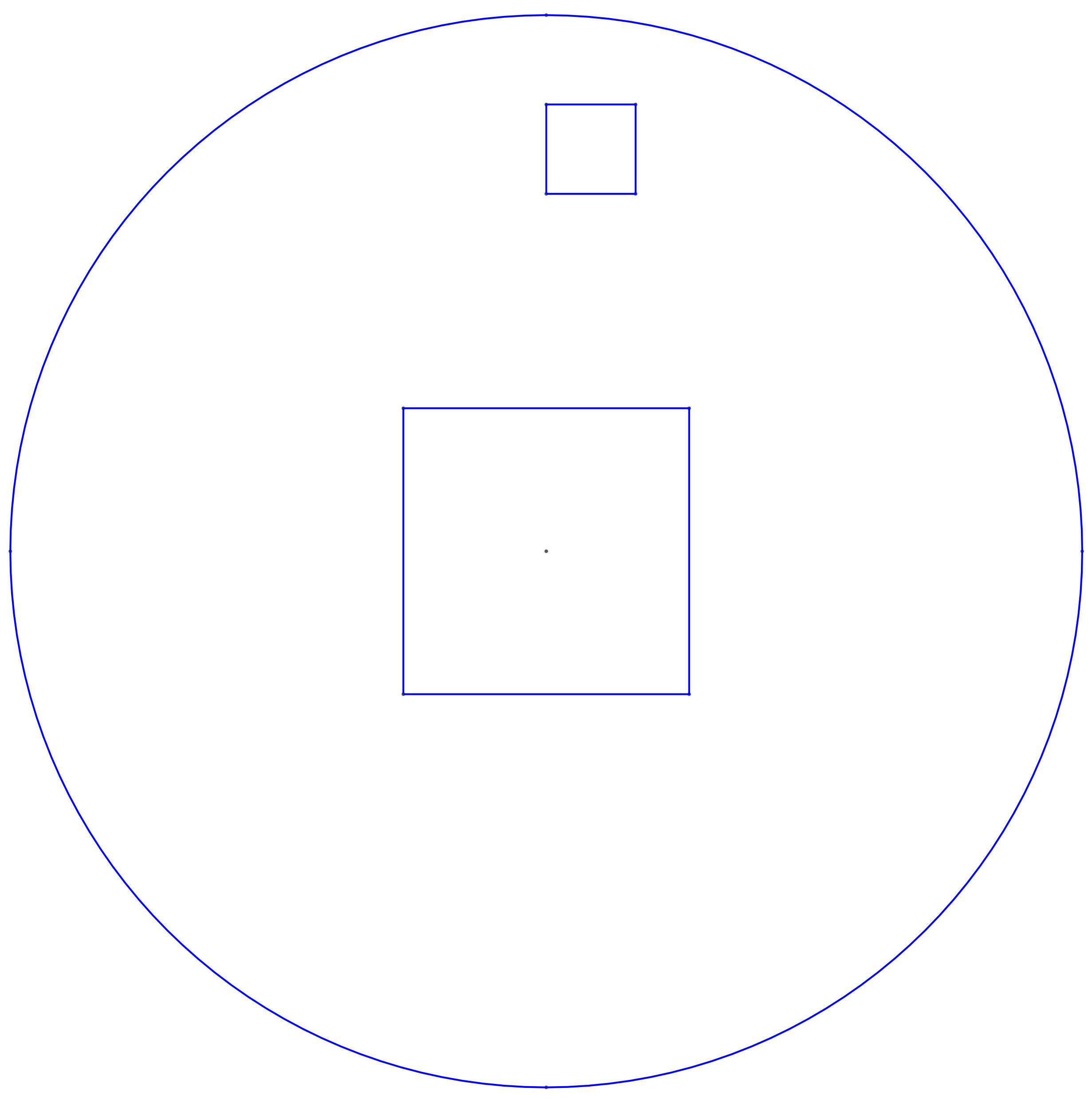 Figure 1
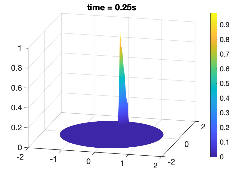 Figure 2
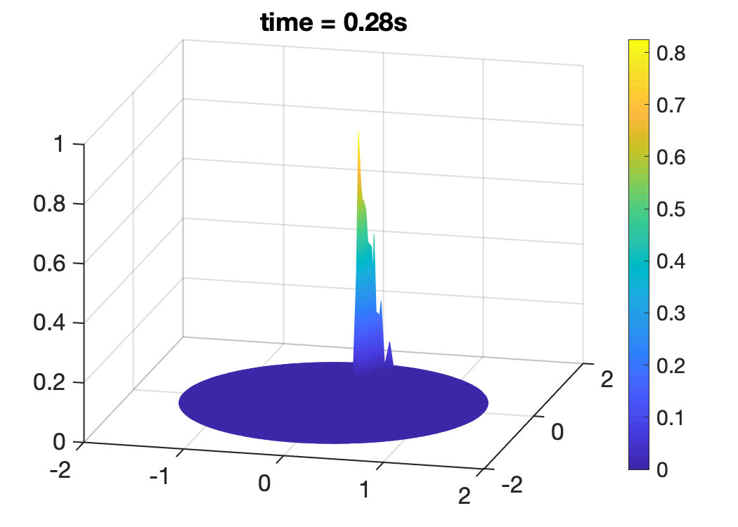 Figure 3
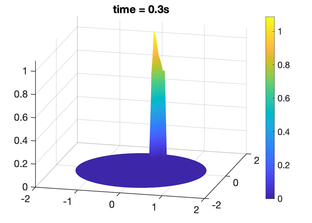 Figure 4
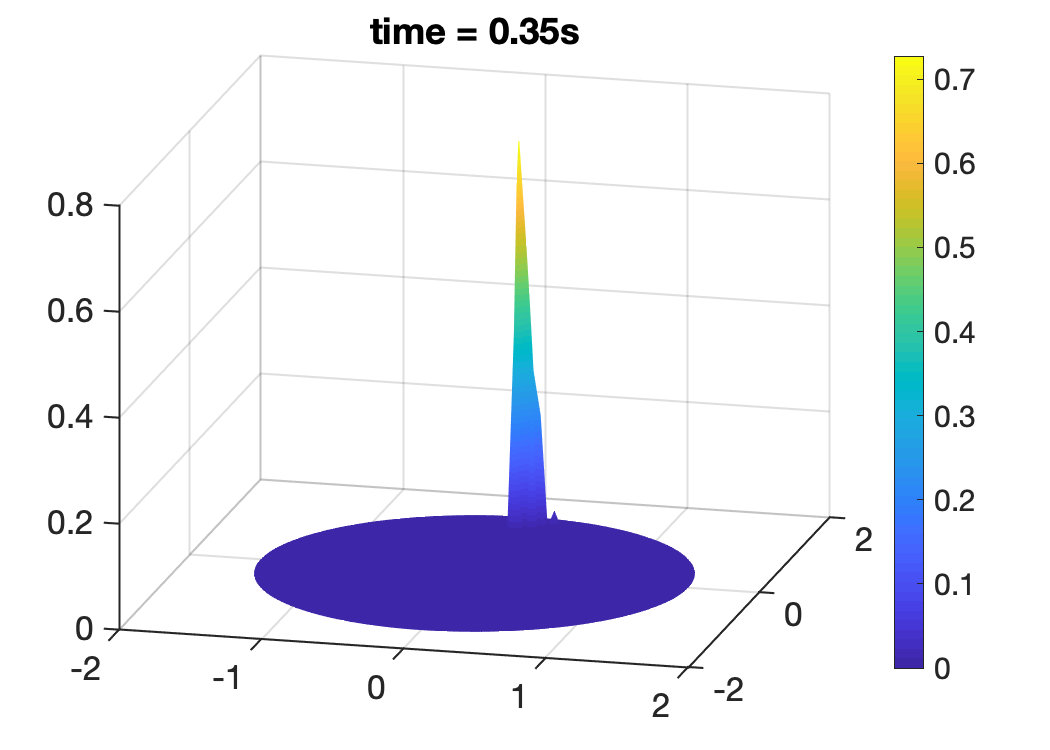 Figure 5
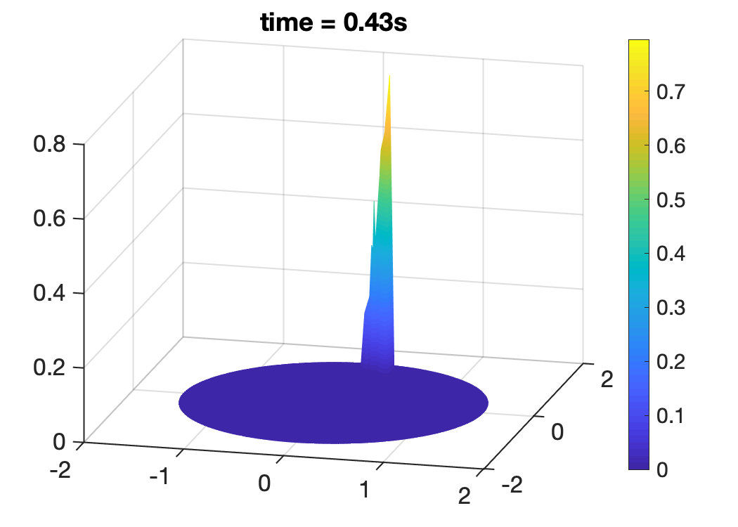 Figure 6
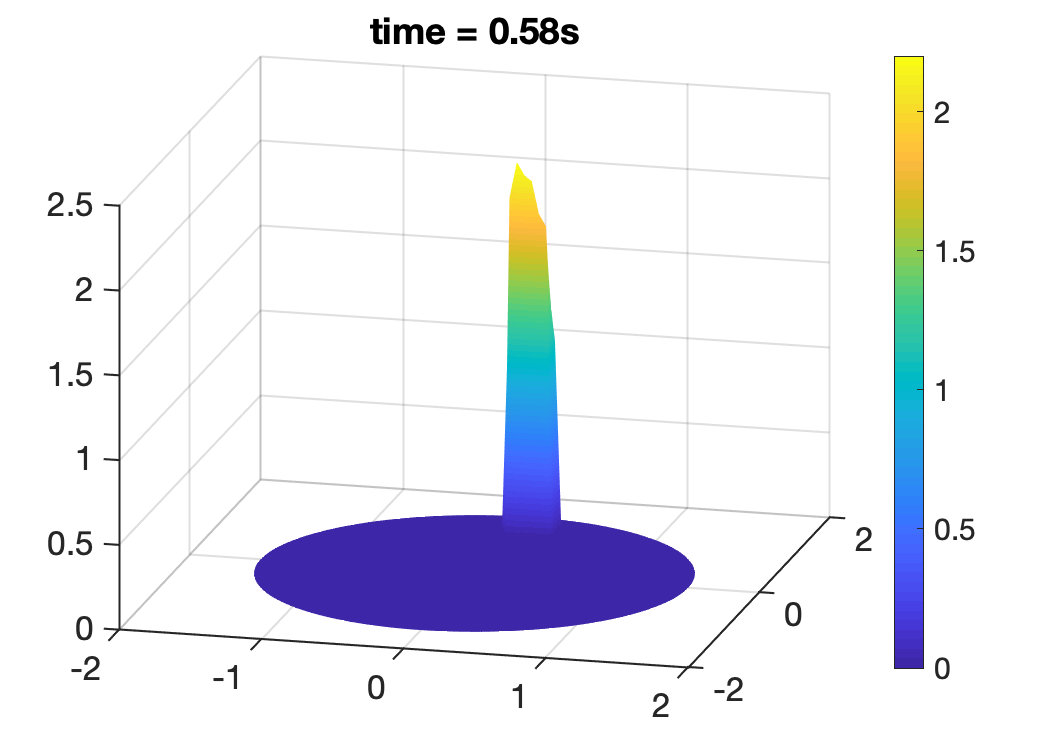 Figure 7
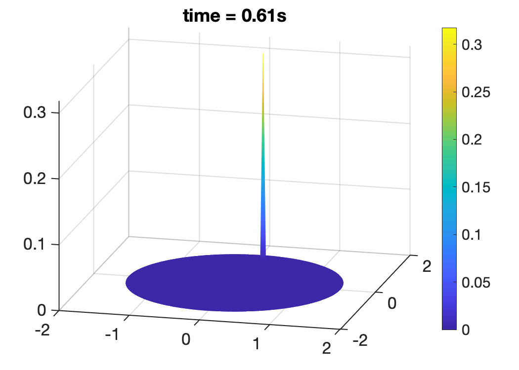 Figure 8
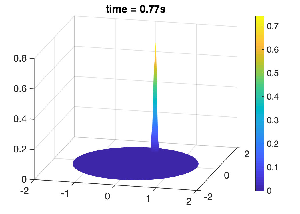 Figure 9
 Figure 10
 Figure 11
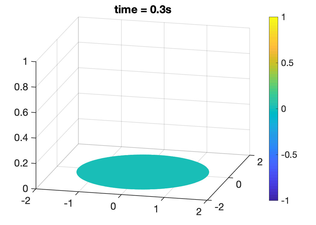 Figure 12
 Figure 13
 Figure 14
 Figure 15
 Figure 16
 Figure 17
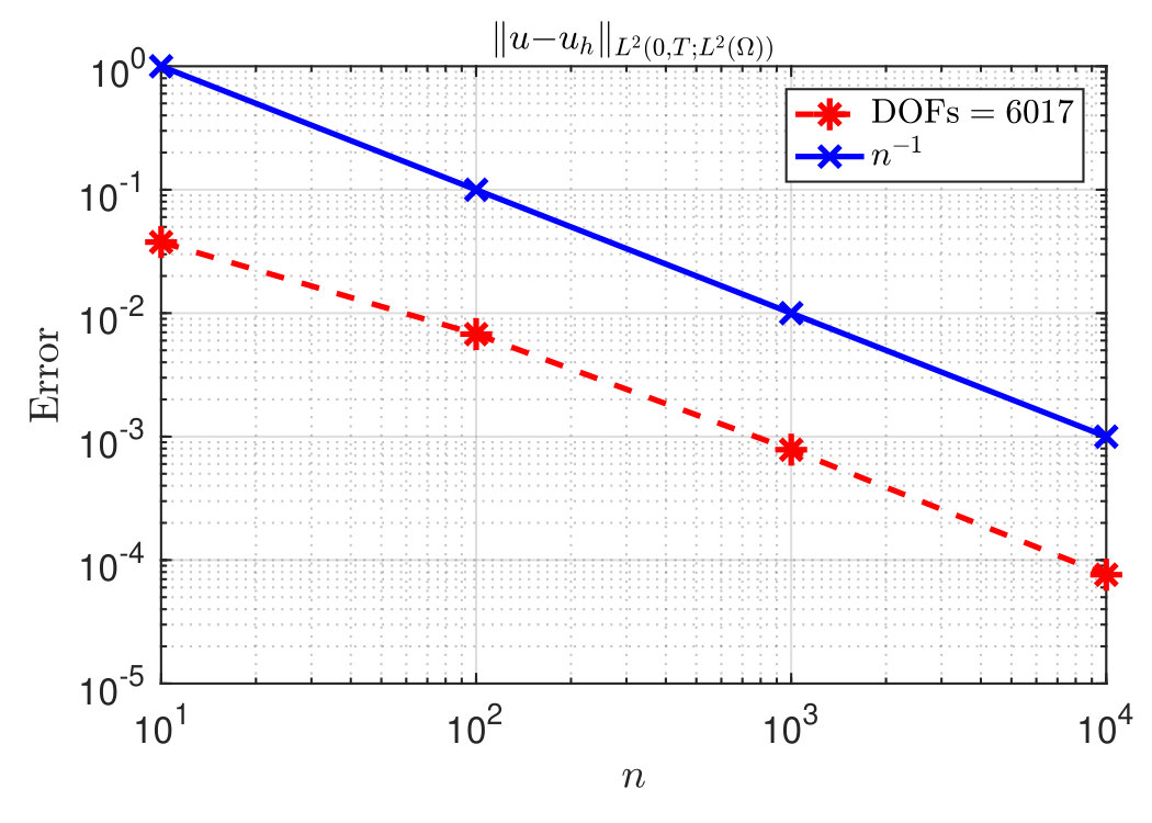 Figure 18
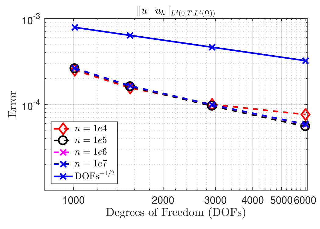 Figure 19
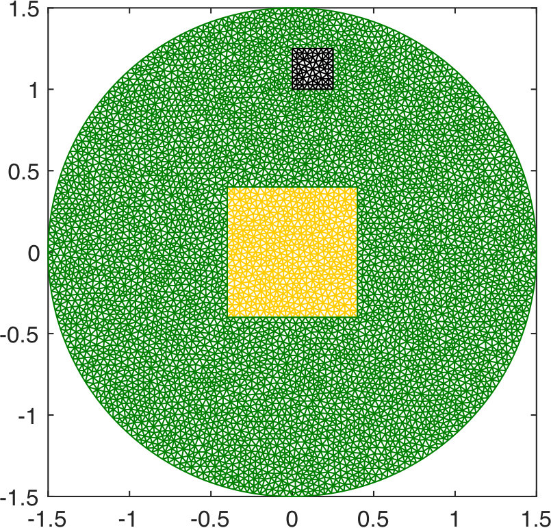 Figure 20
Peer Reviews
No public reviews on file for this paper yet. If you reviewed it on a platform where reviews are public (OpenReview, ICLR, NeurIPS, ICML), you can paste yours below so the community can read it here.
Videos
No videos yet. Explain this paper in a talk, walkthrough, or lecture? Add one.
External optimal control of fractional parabolic PDEs
Harbir Antil
Department of Mathematical Sciences, George Mason University, Fairfax, VA 22030, USA.
,
Deepanshu Verma
Department of Mathematical Sciences, George Mason University, Fairfax, VA 22030, USA.
and
Mahamadi Warma
University of Puerto Rico (Rio Piedras Campus), College of Natural Sciences, Department of Mathematics, PO Box 70377 San Juan PR 00936-8377 (USA).
[email protected], [email protected]
Abstract.
In this paper we introduce a new notion of optimal control, or source identification in inverse, problems with fractional parabolic PDEs as constraints. This new notion allows a source/control placement outside the domain where the PDE is fulfilled. We tackle the Dirichlet, the Neumann and the Robin cases. For the fractional elliptic PDEs this has been recently investigated by the authors in [5]. The need for these novel optimal control concepts stems from the fact that the classical PDE models only allow placing the source/control either on the boundary or in the interior where the PDE is satisfied. However, the nonlocal behavior of the fractional operator now allows placing the control in the exterior. We introduce the notions of weak and very-weak solutions to the parabolic Dirichlet problem. We present an approach on how to approximate the parabolic Dirichlet solutions by the parabolic Robin solutions (with convergence rates). A complete analysis for the Dirichlet and Robin optimal control problems has been discussed. The numerical examples confirm our theoretical findings and further illustrate the potential benefits of nonlocal models over the local ones.
Key words and phrases:
Parabolic PDEs, Fractional Laplacian, weak and very-weak solutions, Dirichlet, Neumann, and Robin external control problems.
2010 Mathematics Subject Classification:
49J20, 49K20, 35S15, 65R20, 65N30
The first and second authors are partially supported by NSF grants DMS-1521590, DMS-1818772 and the Air Force Office of Scientific Research under Award NO: FA9550-19-1-0036. The third author is partially supported by the Air Force Office of Scientific Research under Award NO: FA9550-18-1-0242
1. Introduction
Let , , be a bounded open set with boundary . Consider the Banach spaces and , where the subscripts and denote Dirichlet and Robin. The goal of this paper is to study the following parabolic external optimal control (or source identification) problems:
- •
Fractional parabolic Dirichlet exterior control (source identification) problem: Given a constant penalty parameter we consider the minimization problem:
[TABLE]
with being a closed and convex subset.
- •
Fractional parabolic Robin exterior control (source identification) problem: Given a constant penalty parameter we consider the minimization problem
[TABLE]
with being a closed and convex subset. In (1.2b), denotes the interaction operator and is given in (2.5) below, and is non-negative. We notice that the latter assumption is not a restriction since otherwise we can replace throughout by .
Notice that (1.2b) is a generalized exterior value problem and all the details (with minor modifications) transfer to the case when instead of we consider , where denotes the control/source. The resulting optimal control problem is the parabolic Neumann exterior control problem. We mention that, we can also deal with the following more general system:
[TABLE]
In fact, one has to decompose the solution of the above system as , where satisfies (1.2b) and solves the system
[TABLE]
and use some semigroups method (since in that case is given by a semigroup).
The classical parabolic models, such as diffusion equation, are too restrictive. They only allow a source/control placement either inside the domain or on the boundary of the domain . Notice that in both (1.1b) and (1.2b) the source/control is placed in the exterior domain , disjoint from . This is not possible using the classical models. The authors in [5] have recently introduced the notion of exterior optimal control with elliptic fractional PDEs as constraints. The current paper develops a complete theoretical framework for the parabolic case. The paper [5] has been inspired by the work of M. Warma [46] where the author has shown that the classical notion of controllability (for fractional PDEs) from the boundary does not make sense and therefore it must be replaced by a control that is localized outside the open set where the PDE is solved. For completeness, we would like to mention that the authors have recently considered the case where the source/control is located in the interior [12], see also [11, 13] for the case when the source/control is the diffusion coefficient. We also mention the works on the interior control in case of the so-called spectral fractional Laplacian [9, 12] and for boundary control see [8]. We also mention some interesting but (not directly related) works on fractional Calderón type inverse problems [28, 34, 41]. Notice that fractional operators further provide flexibility to approximate arbitrary functions [23, 26, 31, 33].
The key difficulties and novelties of this paper are as follows:
- (i)
Nonlocal diffusion operator and exterior conditions. The fractional Laplacian is a nonlocal operator and its evaluation at a point requires information over the entire . In addition, may be nonsmooth even if is smooth (see e.g. [40, Remark 7.2]). Moreover, we do not have the notion of boundary conditions, but the exterior conditions on . 2. (ii)
Nonlocal normal derivative. is the nonlocal normal derivative of . This can be thought of as a restricted fractional Laplacian in . It is a very difficult object to handle both at the continuous and at the discrete levels. Indeed, the best known regularity result for is given in Lemma 2.2 which says that globally for . Higher regularity results are currently unknown. 3. (iii)
Approximation of Dirichlet problem by Robin. In case of the parabolic Dirichlet problem (1.1), it is imperative to deal with . Indeed, we need to approximate the very-weak solution to the parabolic Dirichlet problem (1.1b) which requires computing of the test functions (see (3.13)). Moreover, the optimality system for the parabolic Dirichlet control problem (1.1) requires an approximation of the of the adjoint variable (see (4.4)). We circumvent the first difficulty by approximating the parabolic Dirichlet problem (1.1b) by a parabolic Robin problem. We also prove a rate of convergence for this approximation. Under this new setup, the first order optimality conditions do not require an approximation of the of the adjoint variable. 4. (iv)
Weak and very-weak solutions. We study the notion of weak-solutions to the parabolic Dirichlet problem (1.1b) which require a higher regularity on the datum . Since for the control problem (1.1) we only assume that , therefore we also develop an even weaker notion of solutions to (1.1b). We call it very-weak solutions. We also develop the notion of weak-solutions to the Robin problem (1.2b) and prove their existence and uniqueness. 5. (v)
Optimal control problems. We establish the well-posedness of solutions to both parabolic Dirichlet and the parabolic Robin control problems.
Models with fractional derivatives are becoming increasing popular which can be attributed to their role in many applications. These models appear in (but not limited to) image denoising, image segmentation and phase field modeling [2, 3, 10]; data analysis and fractional diffusion maps [4]; magnetotellurics (geophysics) [47].
In many realistic applications, the source/control is placed outside the domain where a PDE is fulfilled. Some examples of problems where this may be of relevance are: (a) Magnetic drug delivery: the drug with ferromagnetic particles is injected in the body and external magnetic field is used to steer it to a desired location [6, 7, 38]; (b) Acoustic testing: the aerospace structures are subjected to sound from the loudspeakers [35].
The rest of the paper is organized as follows. We begin with Section 2 which introduces the notations and some preliminary results. The content of this section is well-known. Our main work starts from Section 3 where we first study the notion of weak and very weak solutions to the parabolic Dirichlet problem in Section 3.1. This is followed by the notion of weak solution to the Robin problem in Section 3.2. The emphasis of Section 4 is on the parabolic Dirichlet and the parabolic Robin optimal control problems. In Section 5, we discuss the approximation of the parabolic Dirichlet problem and parabolic Dirichlet control problem by the parabolic Robin ones. Finally, in Section 6 we discuss the numerical approximations of all the problems. The numerical experiments confirm our theoretical estimates. The experiments on the control/source identification problem illustrate the strength of nonlocal approach over the local ones.
2. Notation and Preliminaries
The purpose of this section is to introduce the notations and some preliminary results. The results of this section are well-known. We follow the notation from [5, 46]. Unless otherwise stated, () is a bounded open set and . Let
[TABLE]
and we endow it with the norm defined by
[TABLE]
In order to study the Dirichlet problem (1.1b) we also need to define
[TABLE]
In this case
[TABLE]
defines an equivalent norm on .
The dual spaces of and are denoted by and , respectively. Moreover, shall denote their duality pairing whenever it is clear from the context.
The local fractional order Sobolev space is defined as
[TABLE]
If , then we shall denote by .
Finally, we are ready to introduce the fractional Laplace operator. We set
[TABLE]
and for and , we let
[TABLE]
where the normalized constant is given by
[TABLE]
and is the usual Euler Gamma function (see, e.g. [18, 20, 21, 22, 24, 44, 45]). Then the fractional Laplacian is defined for by the formula
[TABLE]
provided that the limit exists. We remark that it has been shown in [19, Proposition 2.2] that for , we have that
[TABLE]
This is where the constant plays a crucial role.
Now, we define the operator in as follows.
[TABLE]
Then is the realization in of the fractional Laplace operator with the Dirichlet exterior condition in . The following result is well-known (see e.g. [17, 42]).
Proposition 2.1**.**
The operator has compact resolvent and generates a strongly continuous semigroup on .
Next, for we define the nonlocal normal derivative as follows:
[TABLE]
We shall call the interaction operator. Notice that the origin of the term “interaction” goes back to [27]. Clearly is a nonlocal operator and it is well defined on as we discuss next.
Lemma 2.2**.**
The interaction operator maps continuously into . As a result, if , then .
Despite the fact that is defined on , it is still known as the “normal” derivative. This is due to its similarity with the classical normal derivative [5, Proposition 2.2]. We conclude this section by stating the integration by parts formula for the fractional Laplacian (see e.g. [25]).
Proposition 2.3** **(The integration by parts formula for ).
Let be such that . Then for every we have that
[TABLE]
where .
3. The parabolic state equations
Before analyzing the optimal control problems (1.1) and (1.2), for a given function , we shall focus on the Dirichlet (1.1b) and Robin (1.2b) exterior value problems. We shall assume that is a bounded domain with a Lipschitz continuous boundary.
3.1. The parabolic Dirichlet problem for the fractional Laplacian
Let us consider the following auxiliary problem at first
[TABLE]
i.e., a fractional parabolic equation with nonzero right-hand-side but zero exterior condition. Notice that (3.1) can be rewritten as the following Cauchy problem:
[TABLE]
We next state the notion of a weak solution to (3.1):
Definition 3.1** **(Weak solution: homogeneous Dirichlet case).
Let . A is said to be a weak solution to (3.1) if
[TABLE]
for every and almost every .
Remark 3.2**.**
A weak solution to (3.1) belongs to (see [36, Remark 9] for details). **
The existence and uniqueness of solution to (3.1) was shown in [36, Theorem 26].
Proposition 3.3** **(Weak solution to (3.1)).
Let . Then there exists a unique weak solution to (3.1) in the sense of Definition 3.1 given by
[TABLE]
where is the semigroup mentioned in Proposition 2.1. In addition there is a constant such that
[TABLE]
We next introduce the notion of weak solution to our nonhomogeneous problem (1.1b). Notice the higher regularity requirement on the datum .
Definition 3.4** **(Weak solution: nonhomogenous Dirichlet case).
*Let the function
and be such that . Then a is said to be a weak solution to (1.1b) if and*
[TABLE]
for every and almost every .
Towards this end, we show the well-posedness of (1.1b).
Theorem 3.5** **(Weak solution to (1.1b)).
Let be given. Then there exists a unique weak solution to (1.1b) in the sense of Definition 3.4. In addition there is a constant such that
[TABLE]
Proof*.*
Before we proceed with the proof, we need some preparation. Let us first assume that only depends on the spatial variable and consider the -Harmonic extension of that solves the Dirichlet problem
[TABLE]
in a weak sense, i.e., given there exists a unique , such that , solves (3.5) in the sense that
[TABLE]
and there is a constant such that
[TABLE]
The existence of a weak solution to (3.5) and the continuous dependence on data have been shown in [32], see also [29, 43]. When is a function of then it follows from the above arguments that if then . On the other hand, if then .
Now we show the existence of a unique solution to (1.1b) using a lifting argument. We define . Then . Moreover, a simple calculation shows that fulfills
[TABLE]
Since we have assumed that , therefore from the above discussion we have that . Hence, using Proposition 3.1, we get that there exists a unique solving (3.7). Thus the unique solution is given by . It remains to show the estimate (3.4). Firstly, since in , it follows from (3.4) that there is a constant such that
[TABLE]
Secondly, it follows from (3.6) that there is a constant such that
[TABLE]
Thirdly, using (3.8) and (3.9) we get that there is a constant such that
[TABLE]
Since , then using (3.6), we get that
[TABLE]
Note that is a solution of the Dirichlet problem (3.5) with replaced with . This shows that . Hence, using (3.6) again, we obtain that
[TABLE]
Combining (3.1) and (3.1), we get from (3.1) that
[TABLE]
We have shown (3.4) and the proof is finished. ∎
Remark 3.6**.**
Let be the orthonormal basis of eigenfunctions of associated with the eigenvalues . If in Theorem 3.5, one assumes that with , then it has been shown in [46, Theorem 18] that the unique weak solution of (1.1b) is given by
[TABLE]
Our next goal is to reduce the regularity requirements on the datum in both space and time. We shall call the resulting solution as very-weak solution.
Definition 3.7** **(Very-weak solution: nonhomogenous Dirichlet case).
Let the function . A is said to be a very-weak solution to (1.1b) if the identity
[TABLE]
holds for every with , where .
The following result shows the existence and uniqueness of a very-weak solution to (1.1b) in the sense of Definition 3.7. We will prove this result by using a duality argument (see e.g. [30] for the classical case ).
Theorem 3.8**.**
Let . Then there exists a unique very-weak solution to (1.1b) according to Definition 3.7 that fulfills
[TABLE]
for a constant . In addition, if , then the following assertions hold.
- (a)
Every weak solution of (1.1b) is also a very-weak solution. 2. (b)
Every very-weak solution of (1.1b) that belongs to is also a weak solution.
Proof*.*
For a given , we begin by considering the following “dual” problem
[TABLE]
Using semigroup theory as in Proposition 3.3, one can easily deduce that the problem (3.15) has a unique weak solution .
Since , owing to Lemma 2.2, we have that . Towards, this end we define the mapping
[TABLE]
We notice that is linear and continuous because
[TABLE]
Let , then we have
[TABLE]
We have constructed a unique that solves (3.13). Finally, we notice that
[TABLE]
Dividing both sides by and taking the supremum over we obtain (3.14).
Next we prove the last two assertions of the theorem. Assume that .
(a) Let be a weak solution to (1.1b). It follows from the definition that on and
[TABLE]
for every and almost every . Since in , we have that
[TABLE]
Using (3.16), (3.1), the integration by parts formula (2.6) together with the fact that in , we get that
[TABLE]
Thus is a very-weak solution of (1.1b).
(b) Let be a very-weak solution to (1.1b) and assume that . We have that in . Moreover, and if is such that , then clearly . Since is a very-weak solution to (1.1b), then by Definition 3.7, for every with , we have that
[TABLE]
Since , on , using the integration by parts formula (2.6) we get that
[TABLE]
It then follows form (3.18) and (3.1) that for every with we have the identity
[TABLE]
Since is dense in and is dense in , it follows that (3.20) remains true for with . Notice that for every we have that . As a result, we have that the following pointwise formulation
[TABLE]
holds for every which is independent on . We have shown that is the unique weak solution to (1.1b) according to Definition 3.4 and the proof is complete. ∎
3.2. The parabolic Robin problem for the fractional Laplacian
In this section, we shall consider the Robin problem (1.2b). We begin by specifying the Sobolev space as introduced in [25]. Here we follow the notation from [5]. For fixed, we let
[TABLE]
where
[TABLE]
Let be the measure on given by . With this setting, the norm in (3.22) can be rewritten as
[TABLE]
If , we shall let . The following result has been proved in [25, Proposition 3.1].
Proposition 3.9**.**
Let . Then is a Hilbert space.
Throughout the remainder of the paper, the measure is defined with replaced by . That is, (recall that is assumed to be non-negative). We next state our notion of weak solution.
Definition 3.10**.**
Let . A is said to be a weak solution of (1.2b) if the identity
[TABLE]
holds for every and almost every .
Throughout the following, for we shall denote
[TABLE]
Next we show the existence result.
Theorem 3.11**.**
Let . Then for every , there exists a unique weak solution of (1.2b).
Proof*.*
We prove the result in several steps.
Step 1. Define the operator in as follows:
[TABLE]
Let . We claim that with if and only if
[TABLE]
for all . Indeed, we have that with if and only if is a weak solution of the elliptic problem
[TABLE]
It has been shown in [5] (see also [37]) that solves (3.26) if and only if (3.25) holds and the claim is proved.
Step 2. Firstly, let be a real number. We show that the operator is invertible. It is clear that for every there is a constant such that
[TABLE]
for all . Hence by Lax-Milgram Theorem, for every there exists a unique such that
[TABLE]
for all . By Step 1, this means that there is a unique with and
[TABLE]
We have shown that is a bijection for every .
Secondly, assume now that a.e. in and -a.e. in . Let the function and set . It follows from [45] that . Let . Since
[TABLE]
we have that . Hence,
[TABLE]
Then by (3.28), we have that
[TABLE]
By (3.27) this implies that , that is, almost everywhere. We have shown that the resolvent is a positive operator. Since every positive linear operator is continuous (see e.g., [15]), we can deduce that is in fact invertible.
Thirdly, we have in particular shown that the operator is closed since is the operator associated with the closed form . Hence endowed with the graph norm is a Banach space and by definition of , we have that . Since both of these spaces are continuously embedded into , we can deduce from the closed graph theorem that is continuously embedded into .
Step 3. Now since is a Banach lattice with order continuous norm and by Step 2 the operator is resolvent positive, it follows from [14, Theorem 3.11.7] that generates a once integrated semigroup on . Hence using the theory of integrated semigroups and abstract Cauchy problems studied in [14, Section 3.11] and proceeding as in [39, Section 2], we can deduce that for every , the problem (1.2b) has a unique weak solution. The proof is finished. ∎
We conclude this section by showing that if is more regular in the time variable, then the existence of weak solutions can be easily proved without using the theory of integrated semigroups as in the proof of Theorem 3.11.
Proposition 3.12**.**
Let . Then for every , there exists a unique weak solution of (1.2b).
Proof*.*
We proceed as in the proof of Theorem 3.5. First, assume that does not depend on time and . Let be the solution of the elliptic Robin problem
[TABLE]
in the sense that and
[TABLE]
for every . Under our assumptions, it has been shown in [5] that (3.29) has a solution .
Next, assume that . Since in this case will be a solution of (3.29) with replaced by , then we can deduce that (3.29) has a unique solution .
Consider the following parabolic problem
[TABLE]
Let be the realization of with the zero Robin exterior condition in . Then the parabolic problem (3.31) can be rewritten as the following Cauchy problem
[TABLE]
It has been shown in [37] that the operator generates a strongly continuous semigroup in . Hence, using semigroup theory, we can deduce that (3.31) has a unique weak solution that belongs to and is given by
[TABLE]
It is clear that is the unique weak solution of (1.2b). The proof is finished. ∎
4. Exterior Optimal Control Problems
The purpose of this section is study the Dirichlet and the Robin optimal control problems (1.1) and (1.2), respectively. These are the subjects of Sections 4.1 and 4.2, respectively.
4.1. Fractional Dirichlet Exterior Control Problem
We begin by defining the function spaces and . We let
[TABLE]
Due to Theorem 3.8, the control-to-state (solution) map
[TABLE]
is well-defined, linear and continuous. Furthermore, for , we have that . Thus we can write the so-called reduced Dirichlet exterior parabolic optimal control problem as follows:
[TABLE]
Next, we state the well-posedness result for (1.1) and equivalently (4.1).
Theorem 4.1**.**
Let be a closed and convex subset of . Let either or be bounded and let be weakly lower-semicontinuous. Then there exists a solution to (4.1) and equivalently (1.1). If either is convex and or is strictly convex and , then is unique.
Proof*.*
The proof is based on the so-called direct method or the Weierstrass theorem [16, Theorem 3.2.1]. We sketch the proof here for completeness. For the functional , it is possible to construct a minimizing sequence (see [16, Theorem 3.2.1]) such that . If or is bounded, then is a bounded sequence in which is a Hilbert space. As a result, we have that (up to a subsequence if necessary) (weak convergence) in as . Finally since is closed and convex, hence is weakly closed, we have that .
It then remains to show that fullfills the state equation according to Definition 3.7 and is a minimizer to (4.1). In order to show that fulfills the state equation, we need to focus on the identity
[TABLE]
for all with and for a.e. , as . Since in as and in as , we can immediately take the limit and conclude that fulfills the state equation according to Definition 3.7.
Next, that is the minimizer of (4.1) follows from the fact that is weakly lower semicontinuous: is the sum of two weakly lower semicontinuous functions (recall that the norm is continuous and convex therefore weakly lower semicontinuous).
Finally, uniqueness of follows from the stated assumptions on and which leads to strict convexity of . The proof is finished. ∎
In order to derive the first order necessary optimality conditions, we need an expression of the adjoint operator . We discuss this next. We notice that for every measurable set , we have that with equivalent norms.
Lemma 4.2**.**
The adjoint operator for the state equation (1.1b) is given by
[TABLE]
where and is the weak solution to the problem
[TABLE]
Proof*.*
First of all, since is linear and bounded, it follows that is well-defined. Now for every and , we have that
[TABLE]
Next, testing the equation (4.3) with which solves the state equation in the very-weak sense (cf. Definition 3.13) we obtain that
[TABLE]
and the proof is complete. ∎
For the remainder of this section, we will assume that .
Theorem 4.3**.**
Let be open such that and let the assumptions of Theorem 4.1 hold. Moreover, let be continuously Fréchet differentiable with . If is a minimizer of (4.1) over , then the first order necessary optimality conditions are given by
[TABLE]
where solves the adjoint equation
[TABLE]
Finally, (4.4) is equivalent to
[TABLE]
where is the projection onto the set . Moreover, if is convex then (4.4) is a sufficient condition.
Proof*.*
The statements are a direct consequence of the differentiability properties of and the chain rule, combined with Lemma 4.2. Indeed, let be given, then the directional derivative of is given by
[TABLE]
where we have used that . Using Lemma 4.2, the proof of the first part is finished. Finally, using Lemma 2.2 we have that . Then (4.6) follows by using [16, Theorem 3.3.5]. The proof is finished. ∎
4.2. Fractional Robin Optimal Control Problem
Next we shall focus on the Robin optimal control problem (1.2). We let
[TABLE]
Recall that with . Due to Theorem 3.11, the following control-to-state (solution) map
[TABLE]
is well-defined. In addition, is linear and continuous. Owing to the continuous embedding we can instead define
[TABLE]
The so-called reduced Robin exterior parabolic optimal control problem is then given by
[TABLE]
The following well-posedness result holds.
Theorem 4.4**.**
Let be a convex and closed subset of and let either or be bounded. In addition, if is weakly lower-semicontinuous then there exists a solution to (4.7) and equivalently (1.2). If either is convex and or is strictly convex and then is unique.
Proof*.*
The proof is similar to the proof of Theorem 4.1. We only discuss the part where is a minimizing sequence such that in as . Let , , be the solution of (1.2b). We need to show that this sequence converges to in as and solves (1.2b) in the weak sense (cf. Definition 3.10). Since solves (1.2b), we have that the identity
[TABLE]
holds for every and a.e. , where is as defined in (3.30). We note that the mapping is bounded due to Theorem 3.11. As a result, after a subsequence, if necessary, we have that in as . Then taking the limit as in (4.8) we obtain that
[TABLE]
i.e., solves (1.2b) in the weak sense (cf. Definition 3.10). The proof is finished. ∎
As in the previous section, before we state the first order optimality conditions, we shall derive the expression of the adjoint operator .
Lemma 4.5**.**
The adjoint operator is given by
[TABLE]
where and is the weak solution to
[TABLE]
Proof*.*
Let and . Since , with the embedding being continuous, we can write
[TABLE]
Furthermore, testing (4.9) with we obtain that
[TABLE]
where have used the integration-by-parts in both space and time and the fact that solves the state equation according to Definition 3.10. The proof is complete. ∎
We conclude this section with the following first order optimality conditions result whose proof is similar to the Dirichlet case and is omitted for brevity. We shall assume that .
Theorem 4.6**.**
Let be open such that and let the assumptions of Theorem 4.4 holds. Let be continuously Fréchet differentiable with . If is a minimizer of (4.7), then the first order necessary optimality conditions are given by
[TABLE]
where solves the adjoint equation
[TABLE]
Moreover, (4.10) is equivalent to
[TABLE]
where is the projection onto the set . If is convex then (4.10) is sufficient.
5. Approximation of Dirichlet Exterior Value and Control Problems
Recall that the Dirichlet control problem requires approximations of the nonlocal normal derivative of the test function (cf. (3.13)) and the nonlocal normal derivative of the adjoint variable (cf. (4.4)). Nonlocal normal derivative is a delicate object to handle both at the continuous level and at the discrete level. Indeed, the best known regularity result for the nonlocal normal derivative is as given in Lemma 2.2. Moreover, numerical approximation of this object is a daunting task. In order to circumvent the approximations of the nonlocal normal derivative both in (3.13) and (4.4), in this section we propose to approximate the parabolic Dirichlet problem by the following regularized parabolic Dirichlet problem (or the parabolic Robin problem). Subsequently, we shall approximate the parabolic Dirichlet control problem by the regularized parabolic Dirichlet control problem.
Let . In this section we are interested in solutions to the regularized parabolic Dirichlet problem
[TABLE]
that belongs to the space . Notice that the space is endowed with the norm
[TABLE]
Moreover, in our application we shall take such that its support has a positive Lebesgue measure. Thus we make the following assumption.
Assumption 5.1**.**
We assume that and satisfies almost everywhere in , where the Lebesgue measure .
It follows from Assumption 5.1 that .
We recall that a solution to (5.1) belongs to by using Proposition 3.12. In order to show that this solution lies in we recall a result from [5, Lemma 6.2].
Lemma 5.2**.**
[5, Lemma 6.2]** Assume that Assumption 5.1 holds. Then
[TABLE]
defines an equivalent norm on .
We are now ready to state the main result of this section whose proof is motivated by the previously considered elliptic case by the authors in [5].
Theorem 5.3** **(Approximation of weak solutions to Dirichlet problem).
Let Assumption 5.1 hold. Then the following assertions are true.
- (a)
Let and be the weak solution of (5.1). Let be the weak solution to the state equation (1.1b). Then there is a constant (independent of ) such that
[TABLE]
In particular converges strongly to in as . 2. (b)
Let and be the weak solution of (5.1). Then there is a subsequence that we still denote by and a such that in as , and satisfies
[TABLE]
for all with .
Proof*.*
(a) We begin by discussing well-posedness of (5.1). We first notice that under our assumption we have that . Now a weak solution to (5.1) fulfills the identity
[TABLE]
for every and almost every . For every , existence of a unique solution to (5.1) follows by using the arguments of Proposition 3.12.
Next we prove the estimate (5.4). For , we shall let
[TABLE]
It is not difficult to see (cf. [5, Eq. (6.17)]) that there is a constant such that
[TABLE]
Next let be the weak solution to the Dirichlet problem (1.1b) according to Definition 3.4 and let . Using the integration by parts formula (2.6) we get that
[TABLE]
Subsequently letting in (5) and using (5.8) we can conclude that there is a constant (independent of ) such that
[TABLE]
Hence,
[TABLE]
where we have replaced the constant by . Since
[TABLE]
we arrive at
[TABLE]
Then
[TABLE]
which implies that
[TABLE]
In order to obtain (5.4), it then remains to have the estimate .
We notice that with equivalent norms and
[TABLE]
For any let solve the dual problem
[TABLE]
It follows from Proposition 3.3 that there is a unique solution to (5.12) that fulfills
[TABLE]
Notice that and using (5) we obtain that
[TABLE]
Using the preceding identity, (5.10) and (5.13), we obtain that
[TABLE]
Using (5.11) and (5) we get that
[TABLE]
Now the estimate (5.4) follows from (5.10) and (5.15) and the proof of Part (a) is complete.
(b) Let . Using our assumption, we immediately notice that . In addition, satisfies (5). Then similarly to (5.8) we deduce that
[TABLE]
for almost every . Since , we obtain that
[TABLE]
In order to show that is uniformly bounded, we can proceed as in (5.15), i.e., by using a duality argument. Let and be the weak solution of (5.12). Then using (5) and , we obtain
[TABLE]
Then using the above identity, (5.16) and (5.13) we obtain that
[TABLE]
Thus
[TABLE]
Combing (5.16) and (5.18) we get that
[TABLE]
Therefore the sequence is bounded in . Thus, after a subsequence, if necessary, we have that converges weakly to some in as .
It then remains to show (5.5). By (5), for every with we have that
[TABLE]
Next, applying the integration by parts formula (2.6) we can deduce that
[TABLE]
for every with . Combining (5.20) and (5) we get the identity
[TABLE]
for every with . Taking the limit as in (5.22) we obtain that
[TABLE]
for every with . We have shown (5.5) and the proof is finished. ∎
We conclude this section with the approximation of the parabolic Dirichlet control problem (1.1) via the following “regularized” (which is nothing but the Robin control problem) optimal control problem: Let and then
[TABLE]
Theorem 5.4** **(Approximation of the parabolic Dirichlet control problem).
The regularized control problem (5.23) admits a minimizer . If and is bounded then for any sequence with , there exists a subsequence still denoted by such that in and in as with solving the parabolic Dirichlet control problem (1.1) with replaced by .
Proof*.*
The proof is similar to the elliptic case [5] with obvious modifications and has been omitted for brevity. ∎
We conclude this section by writing the stationarity system corresponding to (5.23): Find with in such that
[TABLE]
for all . Here is as in (5.7).
6. Numerical Approximations
In this section, we shall introduce the numerical approximation of all the problems we have considered so far. We remark that solving parabolic fractional PDEs is a delicate issue. One has to assemble the integrals with singular kernels and the resulting system matrices are dense. On the top of that, the optimal control problem requires solving the state equation forward in time and adjoint equation backward in time. This can be prohibitively expensive. The purpose of this section is simply to illustrate that the numerical results are in agreement with the theory and to show the benefits of the fractional optimal control problem.
The rest of the section is organized as follows: In subsection 6.1 we first focus on the approximations of the Robin problem which is same as the regularized Dirichlet problem (5.1). With the help of a numerical example, we illustrate the sharpness of Theorem 5.3. This is followed by a source identification problem in subsection 6.2. The numerical example presented in subsection 6.2 clearly indicates the strength and flexibility of nonlocal problems over the local ones.
6.1. Approximation of parabolic Dirichlet problem by parabolic Robin problem
We begin by introducing a discrete scheme for the parabolic Robin problem (5.1) and recall that we can approximate the parabolic Dirichlet problem by the parabolic Robin problem. Let be an open bounded set that contains , the support of , and the support of . We consider a conforming simplicial triangulation of and such that the resulting partition remains admissible. Throughout we will assume that the support of and are contained in . Let (on ) be the finite element space of continuous piecewise linear functions. We use the backward-Euler to carry out the time discretization: Let denote the number of time intervals, we set the time-step to be , then for , the fully discrete approximation of (5.1) with nonzero right-hand-side and initial datum is given by: find such that
[TABLE]
where is as in (5.7). The approximation of the double integral over is carried out using the approach of [1]. The remaining integrals are computed using quadrature which is accurate for polynomials of degree less than and equal to 4. All the implementations are carried in Matlab and we use the direct solver to solve the linear systems.
We next consider an example of a parabolic Dirichlet problem with nonzero exterior conditions. Let and , we aim to find solving
[TABLE]
The exact solution for this problem is given by
[TABLE]
We set and approximate (6.2) by using (6.1). Moreover, we set . We divide the time interval into 1800 subintervals. For a fixed and spatial Degrees of Freedom (DoFs) , we study the error with respect to in Figure 1 (left). We obtain a convergence rate of , as predicted by Theorem 5.3 (a).
In the right panel, in Figure 1, we have shown the error for a fixed , but , as a function of DoFs. We observe that the error remains stable with respect to as we refine the spatial mesh. Moreover, the observed rate of convergence is .
6.2. Parabolic source/control identification problem
After the validation in the previous example, we are now ready to consider a source/control identification problem where the source/control is located outside the domain . The optimality system is as given in (5.24). The spatial discretization of all the optimization variables is carried out using continuous piecewise linear finite elements and time discretization using backward-Euler. We set the objective function to be
[TABLE]
where is the given data (observations). Moreover, we let where is the support set of the control that is contained in . We solve the optimization problem using projected-BFGS method with Armijo line search.
We consider the domain as given in Figure 2. The circle denotes and the larger square denotes the domain . The smaller square, inside , is is where the source/control is supported. The right panel shows a finite element mesh with DoFs = 6103.
We generate the data as follows: for , we solve the state equation (first equation in (5.24)). We then add a normally distributed noise with mean zero and standard deviation 0.005. We call the resulting expression . In addition, we set and .
Next, we identify the source by solving the optimality system (5.24). For -8, our results are shown in Figure 3. In the first two rows, we have plotted for at 4 time instances . The third row shows for at only one of these time instances since is zero at the remaining three time instances. This is not surprising, since as approaches , the fractional Laplacian approaches the standard Laplacian which does not allow a source placement outside the closure of .
The reference list from the paper itself. Each links out to its DOI / PubMed record.
- 1[1] G. Acosta, F.M. Bersetche, and J.P. Borthagaray. A short fe implementation for a 2d homogeneous dirichlet problem of a fractional laplacian. Computers & Mathematics with Applications , 74(4):784–816, 2017.
- 2[2] H. Antil and S. Bartels. Spectral Approximation of Fractional PD Es in Image Processing and Phase Field Modeling. Comput. Methods Appl. Math. , 17(4):661–678, 2017.
- 3[3] H. Antil, S. Bartels, and G. Dogan. A phase field segmentation model with fractional diffusion for improved boundary regularization. Submitted , 2019.
- 4[4] H. Antil, T. Berry, and J. Harlim. Fractional diffusion maps. ar Xiv preprint ar Xiv:1810.03952 , 2018.
- 5[5] H. Antil, R. Khatri, and M. Warma. External optimal control of nonlocal pdes. Inverse Problems, to appear , 2019.
- 6[6] H. Antil, R.H. Nochetto, and P. Venegas. Controlling the Kelvin force: basic strategies and applications to magnetic drug targeting. Optim. Eng. , 19(3):559–589, 2018.
- 7[7] H. Antil, R.H. Nochetto, and P. Venegas. Optimizing the Kelvin force in a moving target subdomain. Math. Models Methods Appl. Sci. , 28(1):95–130, 2018.
- 8[8] H. Antil, J. Pfefferer, and S. Rogovs. Fractional operators with inhomogeneous boundary conditions: Analysis, control, and discretization. Communications in Mathematical Sciences (CMS) , 16(5):1395–1426, 2018.