Accurate modelling of the low-order secondary resonances in the spin-orbit problem
Ioannis Gkolias, Christos Efthymiopoulos, Alessandra Celletti, and Giuseppe Pucacco

TL;DR
This paper develops an analytical method to accurately model low-order secondary resonances in the spin-orbit problem, enhancing understanding of planetary satellite spin states and bifurcations.
Contribution
It extends a perturbative normal form approach to analytically describe phase space topology and bifurcations of key secondary resonances in the gravitational spin-orbit problem.
Findings
Explicit formulas for secondary resonance dynamics
Characterization of phase portraits and bifurcations
Error estimates for the analytical approximation
Abstract
We provide an analytical approximation to the dynamics in each of the three most important low order secondary resonances (1:1, 2:1, and 3:1) bifurcating from the synchronous primary resonance in the gravitational spin-orbit problem. To this end we extend the perturbative approach introduced in Gkolias et. al. (2016), based on normal form series computations. This allows to recover analytically all non-trivial features of the phase space topology and bifurcations associated with these resonances. Applications include the characterization of spin states of irregular planetary satellites or double systems of minor bodies with irregular shapes. The key ingredients of our method are: i) the use of a detuning parameter measuring the distance from the exact resonance, and ii) an efficient scheme to `book-keep' the series terms, which allows to simultaneously treat all small parameters…
Click any figure to enlarge with its caption.
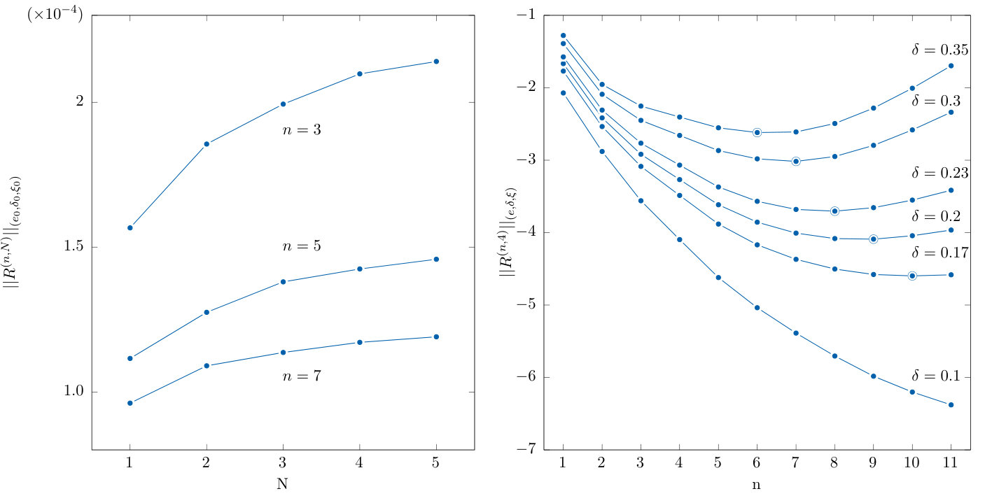 Figure 1
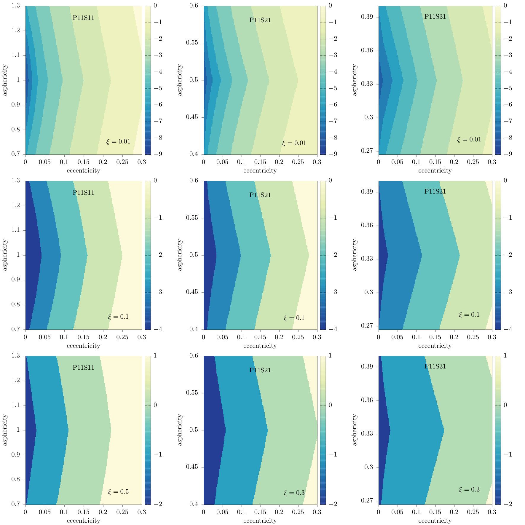 Figure 2
 Figure 3
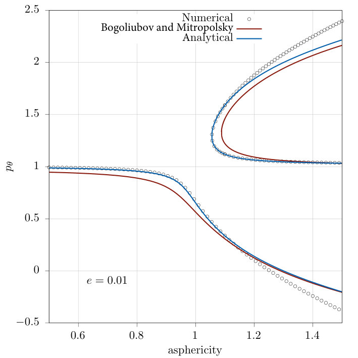 Figure 4
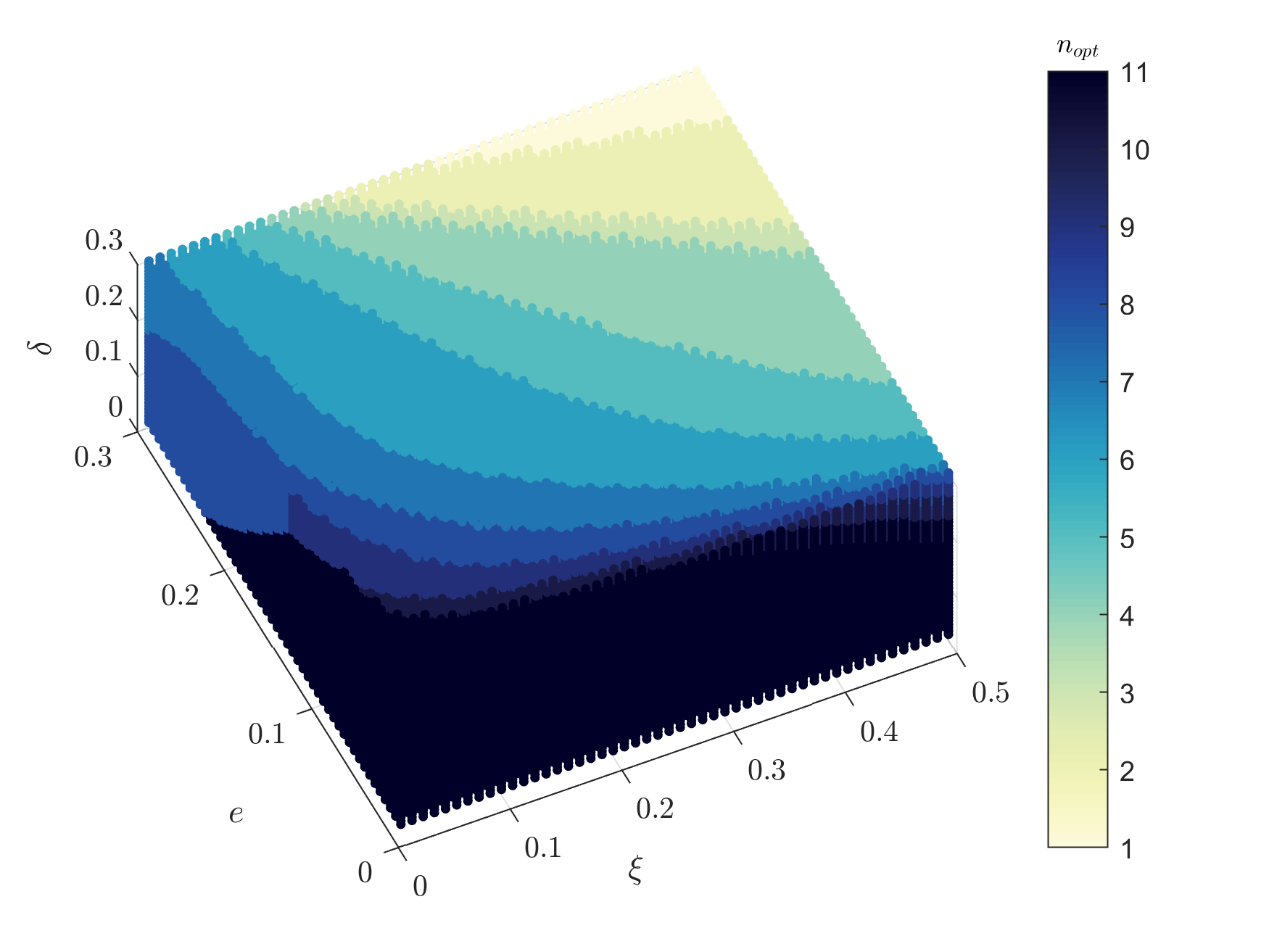 Figure 5
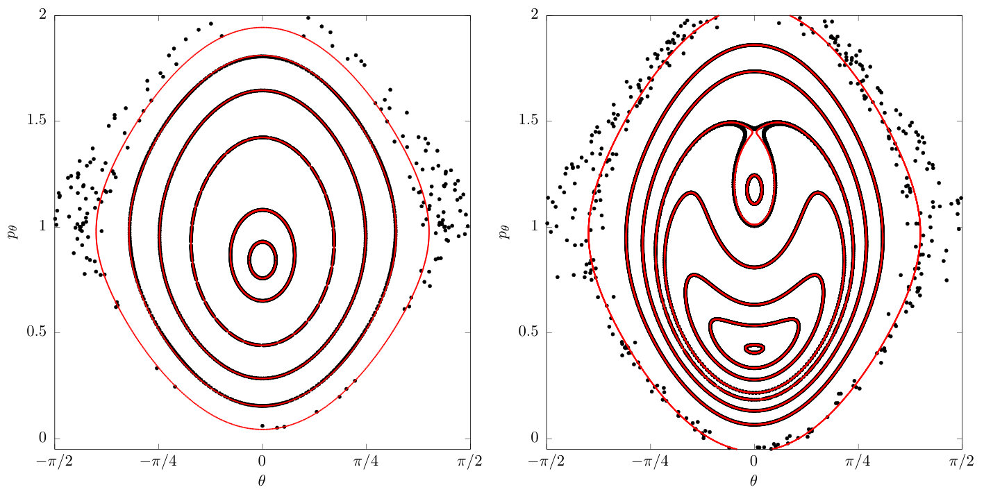 Figure 6
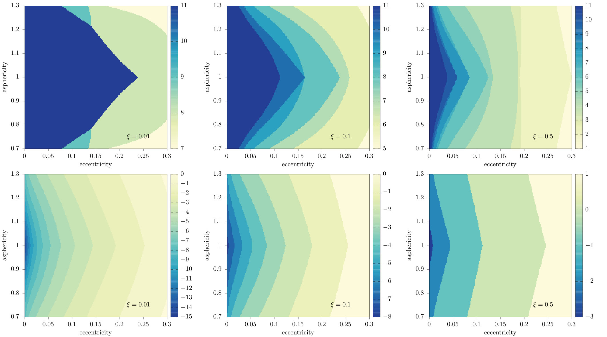 Figure 7
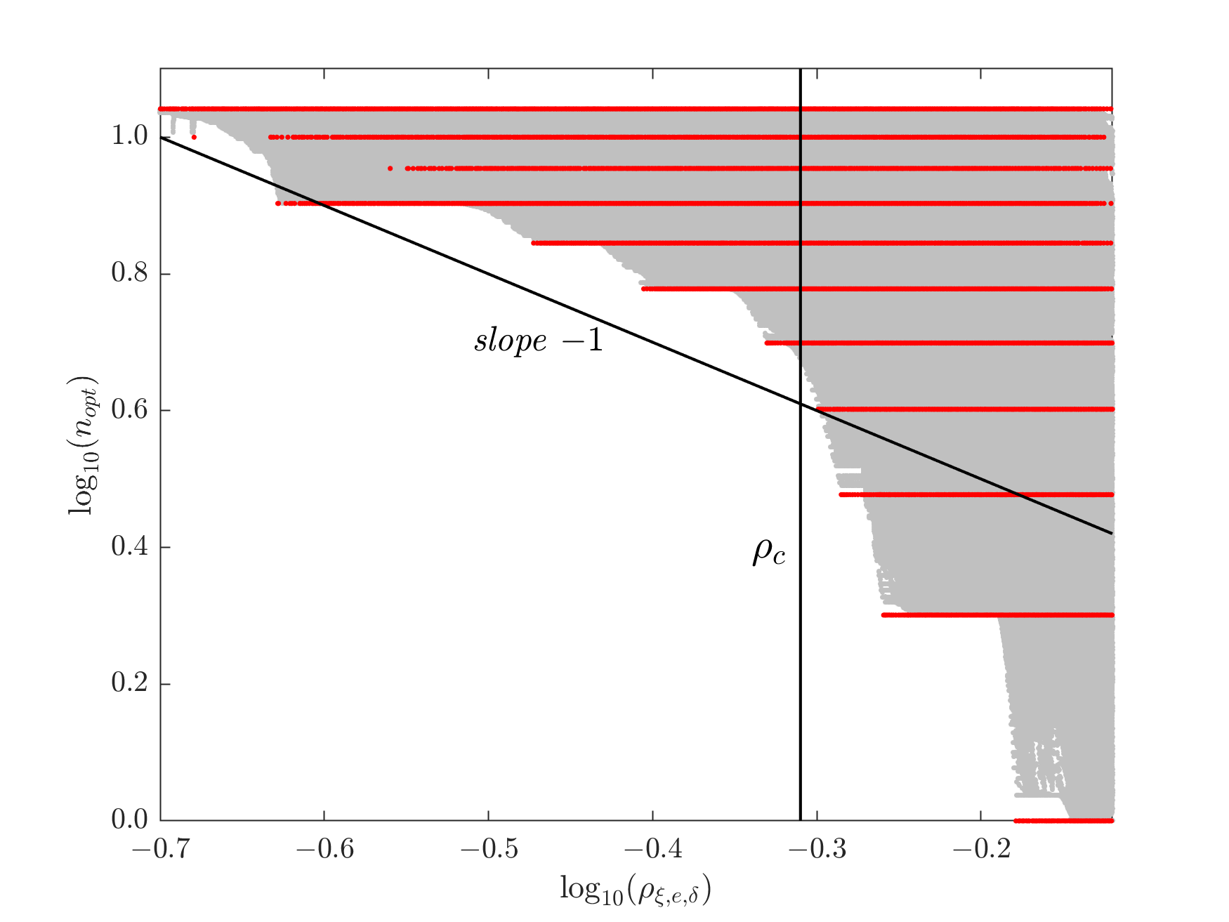 Figure 8
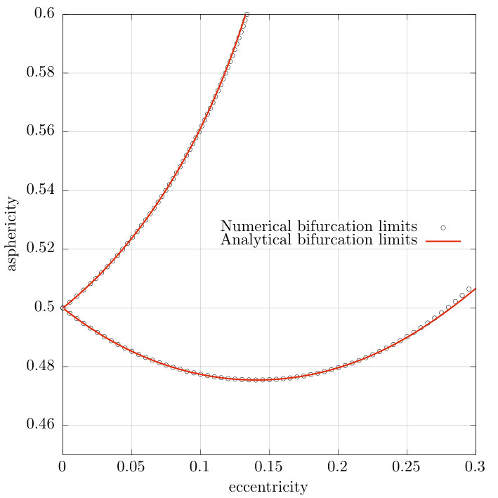 Figure 9
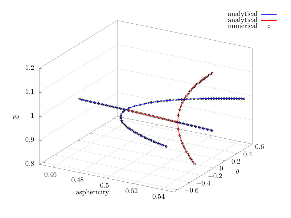 Figure 10
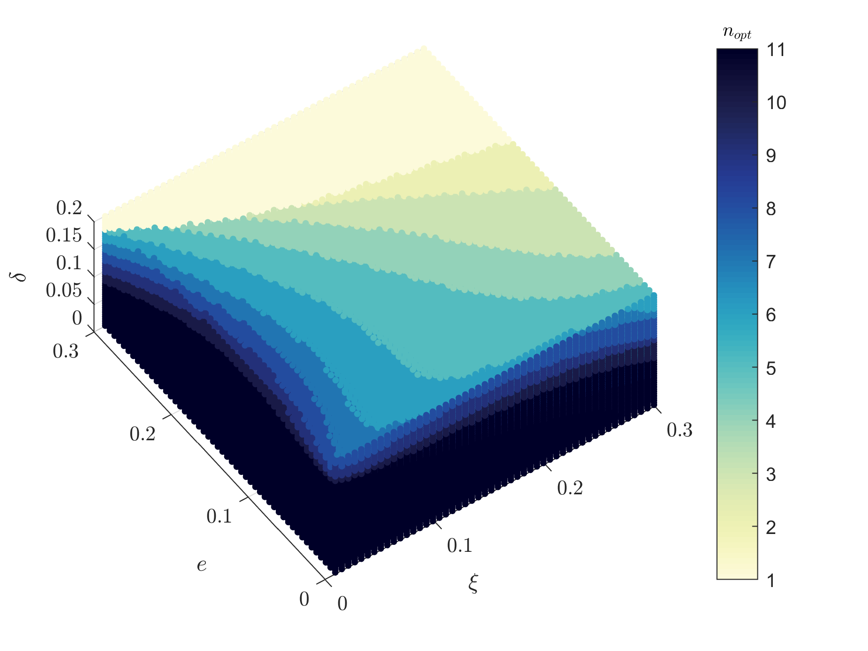 Figure 11
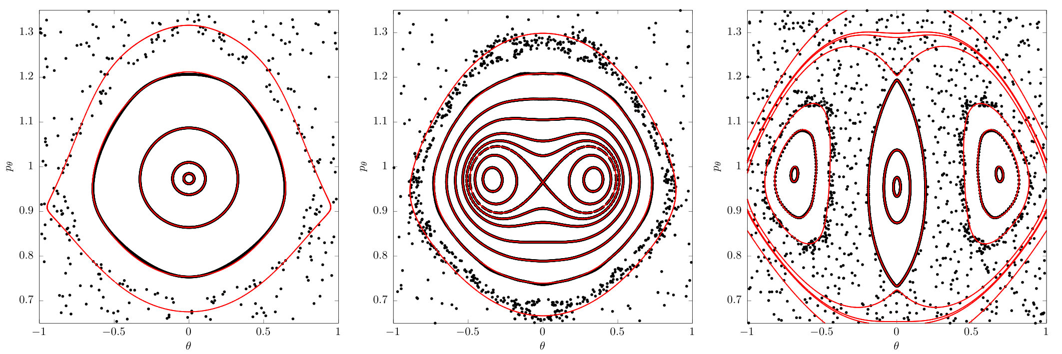 Figure 12
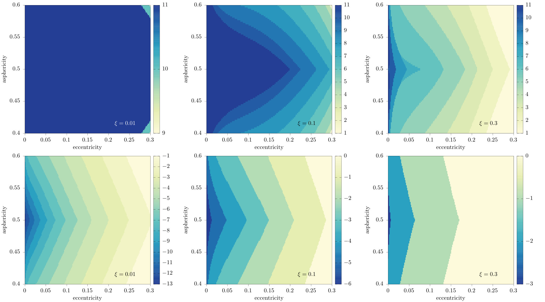 Figure 13
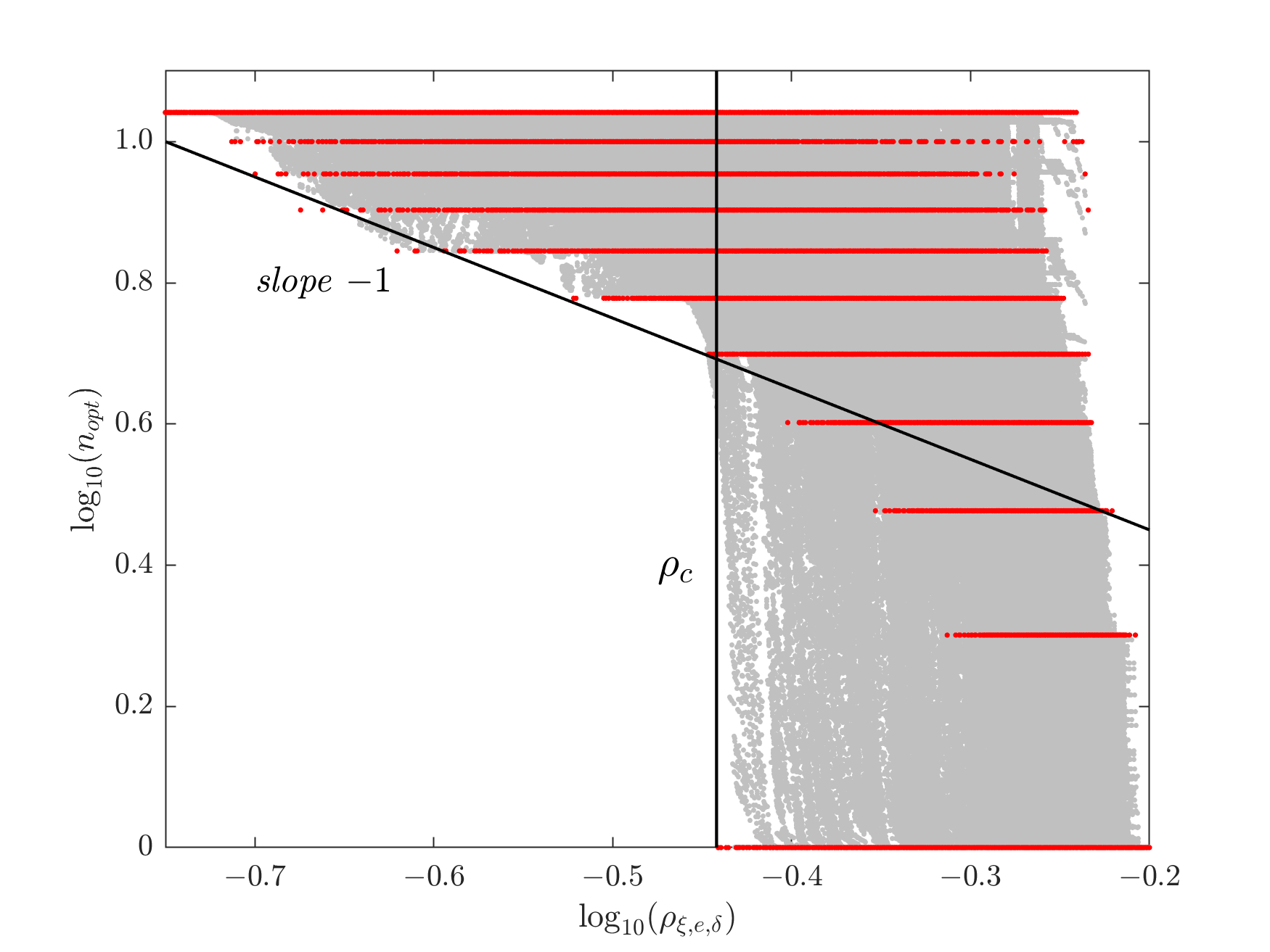 Figure 14
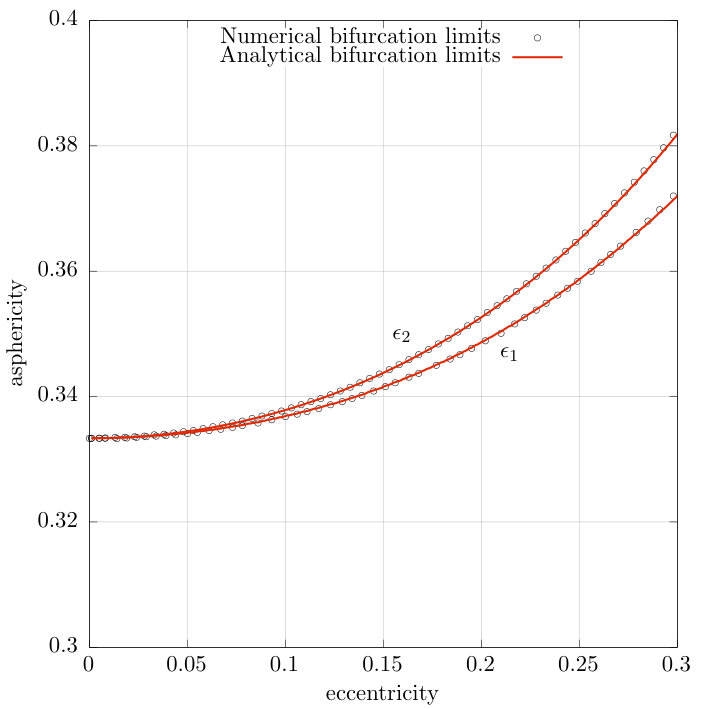 Figure 15
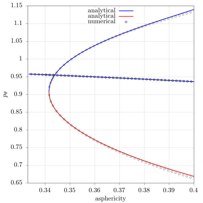 Figure 16
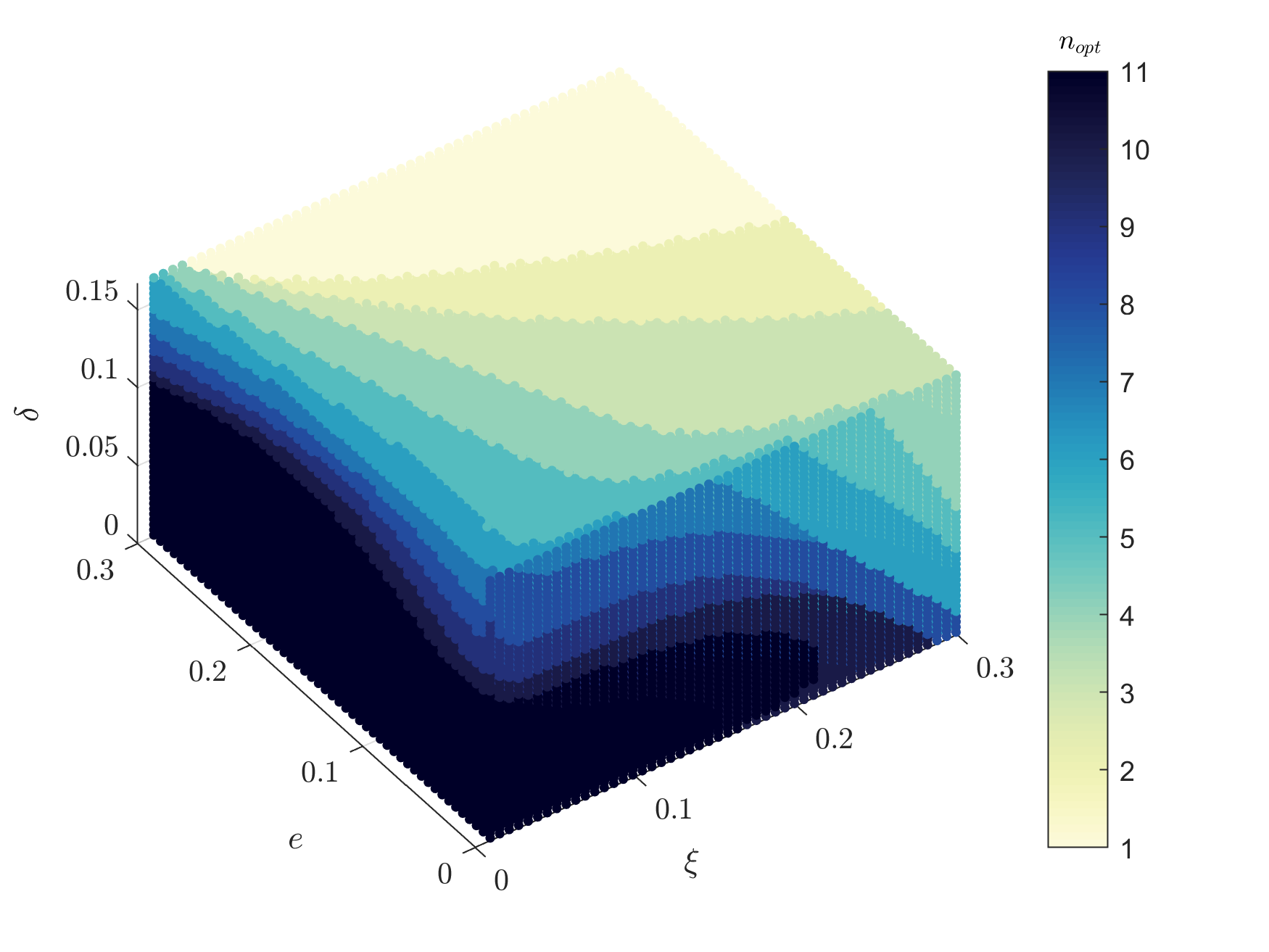 Figure 17
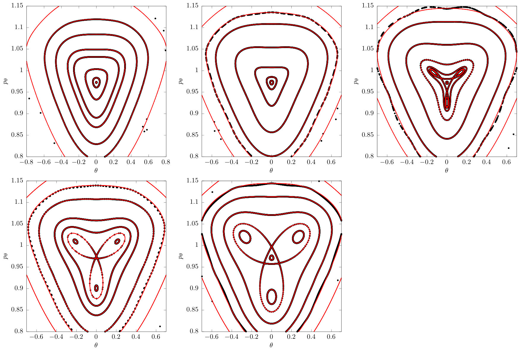 Figure 18
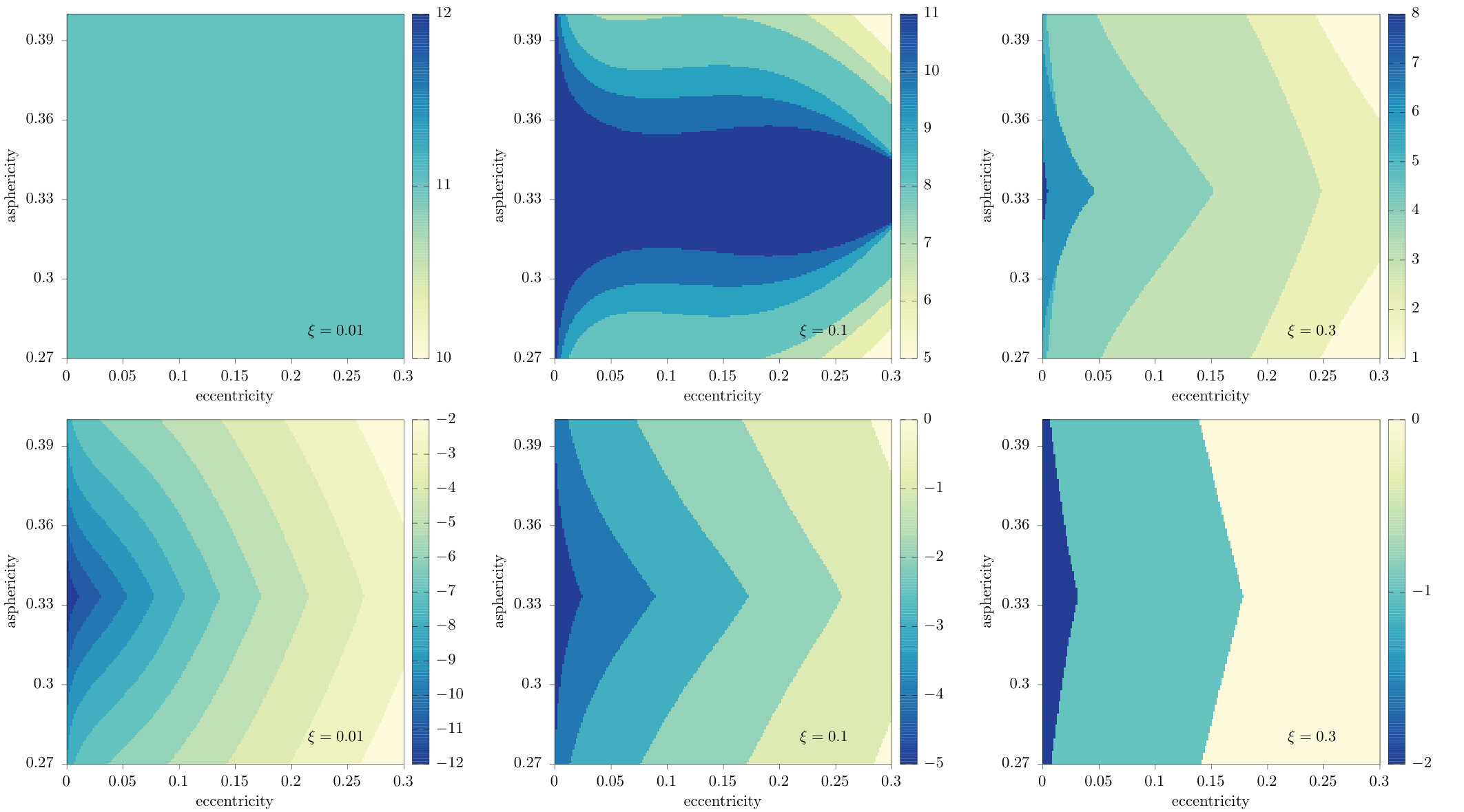 Figure 19
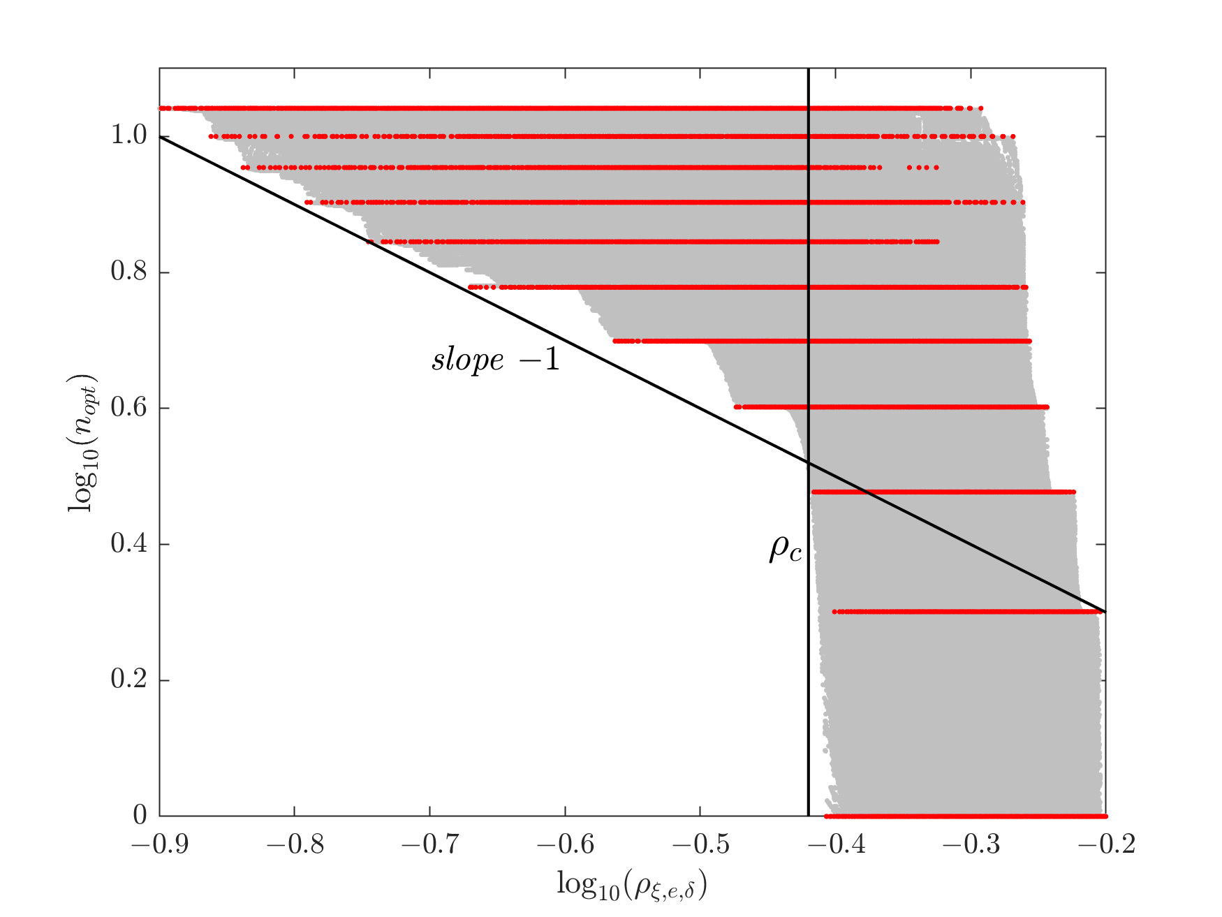 Figure 20
| coeff | |||||
|---|---|---|---|---|---|
| 1 | 0 | 1 | 2 | 0 | 1/2 |
| 1 | 0 | 1 | 2 | 0 | 1/2 |
| 1 | 0 | 1 | 0 | 2 | 1/2 |
| 2 | 2 | 0 | 2 | 0 | -1/2 |
| 2 | 0 | 0 | 4 | 0 | -1/16 |
| 2 | 1 | 0 | 2 | 1 | 1/2 |
| 2 | 2 | 0 | 0 | 2 | -3/2 |
| 2 | 0 | 0 | 2 | 2 | -1/8 |
| 2 | 1 | 0 | 0 | 3 | 1/2 |
| 2 | 0 | 0 | 0 | 4 | -1/16 |
| 3 | 2 | 0 | 2 | 0 | 1/4 |
| 3 | 1 | 0 | 2 | 1 | -1/8 |
| 3 | 2 | 0 | 0 | 2 | 3/4 |
| 3 | 1 | 0 | 0 | 3 | -1/8 |
| 3 | 2 | 1 | 2 | 0 | -1/4 |
| 3 | 1 | 1 | 2 | 1 | 1/4 |
| 3 | 2 | 1 | 0 | 2 | -5/4 |
| 3 | 1 | 1 | 0 | 3 | 1/4 |
| 4 | 2 | 0 | 2 | 0 | -1/32 |
| 4 | 4 | 0 | 2 | 0 | -115/192 |
| 4 | 2 | 0 | 4 | 0 | -9/32 |
| 4 | 0 | 0 | 6 | 0 | -1/128 |
| 4 | 3 | 0 | 2 | 1 | 59/48 |
| 4 | 1 | 0 | 4 | 1 | 3/32 |
| 4 | 2 | 0 | 0 | 2 | -3/32 |
| 4 | 4 | 0 | 0 | 2 | -275/192 |
| 4 | 2 | 0 | 2 | 2 | -3/4 |
| 4 | 0 | 0 | 4 | 2 | -3/128 |
| 4 | 3 | 0 | 0 | 3 | 169/144 |
| 4 | 1 | 0 | 2 | 3 | 3/16 |
| 4 | 2 | 0 | 0 | 4 | -15/32 |
| 4 | 0 | 0 | 2 | 4 | -3/128 |
| 4 | 1 | 0 | 0 | 5 | 3/32 |
| 4 | 0 | 0 | 0 | 6 | -1/128 |
| 4 | 2 | 1 | 2 | 0 | 7/16 |
| 4 | 1 | 1 | 2 | 1 | -5/32 |
| 4 | 2 | 1 | 0 | 2 | 21/16 |
| 4 | 1 | 1 | 0 | 3 | -5/32 |
| 4 | 2 | 2 | 2 | 0 | 25/48 |
| 4 | 1 | 2 | 2 | 1 | -1/16 |
| 4 | 2 | 2 | 0 | 2 | -53/48 |
| 4 | 1 | 2 | 0 | 3 | -1/16 |
| 5 | 4 | 0 | 2 | 0 | 757/384 |
| 5 | 2 | 0 | 4 | 0 | 15/256 |
| 5 | 3 | 0 | 2 | 1 | -673/384 |
| 5 | 1 | 0 | 4 | 1 | -15/512 |
| 5 | 4 | 0 | 0 | 2 | 1607/384 |
| 5 | 2 | 0 | 2 | 2 | 45/128 |
| 5 | 3 | 0 | 0 | 3 | -1757/1152 |
| 5 | 1 | 0 | 2 | 3 | -15/256 |
| 5 | 2 | 0 | 0 | 4 | 75/256 |
| coeff | |||||
|---|---|---|---|---|---|
| 1 | 1 | 0 | 2 | 0 | 3/16 |
| 1 | 1 | 0 | 0 | 2 | -3/16 |
| 1 | 0 | 1 | 2 | 0 | 1/2 |
| 1 | 0 | 1 | 0 | 2 | 1/2 |
| 2 | 2 | 0 | 2 | 0 | -89/256 |
| 2 | 0 | 0 | 4 | 0 | -1/16 |
| 2 | 2 | 0 | 0 | 2 | -89/256 |
| 2 | 0 | 0 | 2 | 2 | -1/8 |
| 2 | 0 | 0 | 0 | 4 | -1/16 |
| 2 | 1 | 1 | 2 | 0 | 3/8 |
| 2 | 1 | 1 | 0 | 2 | -3/8 |
| 3 | 2 | 0 | 2 | 0 | -1/3 |
| 3 | 3 | 0 | 2 | 0 | -365/4096 |
| 3 | 1 | 0 | 4 | 0 | -3/64 |
| 3 | 2 | 0 | 0 | 2 | -1/3 |
| 3 | 3 | 0 | 0 | 2 | 365/4096 |
| 3 | 1 | 0 | 0 | 4 | 3/64 |
| 3 | 2 | 1 | 2 | 0 | -223/256 |
| 3 | 2 | 1 | 0 | 2 | -223/256 |
| 3 | 1 | 2 | 2 | 0 | -3/8 |
| 3 | 1 | 2 | 0 | 2 | 3/8 |
| 4 | 2 | 0 | 2 | 0 | -1/18 |
| 4 | 3 | 0 | 2 | 0 | -31/240 |
| 4 | 4 | 0 | 2 | 0 | 62221/196608 |
| 4 | 2 | 0 | 4 | 0 | 3619/10240 |
| 4 | 0 | 0 | 6 | 0 | -1/64 |
| 4 | 2 | 0 | 0 | 2 | -1/18 |
| 4 | 3 | 0 | 0 | 2 | 31/240 |
| 4 | 4 | 0 | 0 | 2 | 62221/196608 |
| 4 | 2 | 0 | 2 | 2 | -2981/5120 |
| 4 | 0 | 0 | 4 | 2 | -3/64 |
| 4 | 2 | 0 | 0 | 4 | 3619/10240 |
| 4 | 0 | 0 | 2 | 4 | -3/64 |
| 4 | 0 | 0 | 0 | 6 | -1/64 |
| 4 | 2 | 1 | 2 | 0 | -22/9 |
| 4 | 3 | 1 | 2 | 0 | 239/256 |
| 4 | 1 | 1 | 4 | 0 | 15/64 |
| 4 | 2 | 1 | 0 | 2 | -22/9 |
| 4 | 3 | 1 | 0 | 2 | -239/256 |
| 4 | 1 | 1 | 0 | 4 | -15/64 |
| 4 | 2 | 2 | 2 | 0 | -3/256 |
| 4 | 2 | 2 | 0 | 2 | -3/256 |
| 4 | 1 | 3 | 2 | 0 | 13/16 |
| 4 | 1 | 3 | 0 | 2 | -13/16 |
| 5 | 3 | 0 | 2 | 0 | -3/160 |
| 5 | 4 | 0 | 2 | 0 | 186527/115200 |
| 5 | 5 | 0 | 2 | 0 | -458595/1048576 |
| 5 | 2 | 0 | 4 | 0 | 23/120 |
| 5 | 3 | 0 | 4 | 0 | -15443/409600 |
| 5 | 1 | 0 | 6 | 0 | -57/1024 |
| coeff | |||||
|---|---|---|---|---|---|
| 1 | 0 | 1 | 2 | 0 | 1/2 |
| 1 | 0 | 1 | 0 | 2 | 1/2 |
| 2 | 2 | 0 | 2 | 0 | -2/15 |
| 2 | 0 | 0 | 4 | 0 | -1/16 |
| 2 | 1 | 0 | 2 | 1 | 1/(2 ) |
| 2 | 2 | 0 | 0 | 2 | -2/15 |
| 2 | 0 | 0 | 2 | 2 | -1/8 |
| 2 | 1 | 0 | 0 | 3 | -1/(6 ) |
| 2 | 0 | 0 | 0 | 4 | -1/16 |
| 3 | 2 | 0 | 2 | 0 | -1/12 |
| 3 | 1 | 0 | 2 | 1 | 1/(16 ) |
| 3 | 2 | 0 | 0 | 2 | -1/12 |
| 3 | 1 | 0 | 0 | 3 | -1/(48 ) |
| 3 | 2 | 1 | 2 | 0 | 41/100 |
| 3 | 1 | 1 | 2 | 1 | /4 |
| 3 | 2 | 1 | 0 | 2 | 41/100 |
| 3 | 1 | 1 | 0 | 3 | -1/(4 ) |
| 4 | 2 | 0 | 2 | 0 | -1/192 |
| 4 | 4 | 0 | 2 | 0 | -7837/24000 |
| 4 | 2 | 0 | 4 | 0 | -277/1200 |
| 4 | 0 | 0 | 6 | 0 | -3/128 |
| 4 | 3 | 0 | 2 | 1 | -97/(400 ) |
| 4 | 2 | 0 | 0 | 2 | -1/192 |
| 4 | 4 | 0 | 0 | 2 | -7837/24000 |
| 4 | 2 | 0 | 2 | 2 | -277/600 |
| 4 | 0 | 0 | 4 | 2 | -9/128 |
| 4 | 3 | 0 | 0 | 3 | 97/(1200 ) |
| 4 | 2 | 0 | 0 | 4 | -277/1200 |
| 4 | 0 | 0 | 2 | 4 | -9/128 |
| 4 | 0 | 0 | 0 | 6 | -3/128 |
| 4 | 2 | 1 | 2 | 0 | -13/16 |
| 4 | 1 | 1 | 2 | 1 | 11 /64 |
| 4 | 2 | 1 | 0 | 2 | -13/16 |
| 4 | 1 | 1 | 0 | 3 | -11/(64 ) |
| 4 | 2 | 2 | 2 | 0 | 7533/1000 |
| 4 | 1 | 2 | 2 | 1 | -3 /16 |
| 4 | 2 | 2 | 0 | 2 | 7533/1000 |
| 4 | 1 | 2 | 0 | 3 | /16 |
| 5 | 4 | 0 | 2 | 0 | 257/4200 |
| 5 | 2 | 0 | 4 | 0 | 7/384 |
| 5 | 3 | 0 | 2 | 1 | -1201/(11200 ) |
| 5 | 4 | 0 | 0 | 2 | 257/4200 |
| 5 | 2 | 0 | 2 | 2 | 7/192 |
| 5 | 3 | 0 | 0 | 3 | 1201/(33600 ) |
| 5 | 2 | 0 | 0 | 4 | 7/384 |
| 5 | 2 | 1 | 2 | 0 | -11/128 |
| 5 | 4 | 1 | 2 | 0 | -194453/40000 |
| 5 | 2 | 1 | 4 | 0 | -66191/16000 |
| 5 | 0 | 1 | 6 | 0 | 9/128 |
| 5 | 3 | 1 | 2 | 1 | -14981 /16000 |
Peer Reviews
No public reviews on file for this paper yet. If you reviewed it on a platform where reviews are public (OpenReview, ICLR, NeurIPS, ICML), you can paste yours below so the community can read it here.
Videos
No videos yet. Explain this paper in a talk, walkthrough, or lecture? Add one.
Accurate modelling of the low-order secondary resonances
in the spin-orbit problem
Ioannis Gkolias
Department of Aerospace Science and Technology, Politecnico di Milano, Via la Masa 34, 20156 Milan, Italy
,
Christos Efthymiopoulos
Research Center for Astronomy, Academy of Athens, Soranou Efessiou 4, 11527 Athens, Greece
,
Alessandra Celletti
Department of Mathematics, University of Rome Tor Vergata, Via della Ricerca Scientifica 1, 00133 Rome, Italy
and
Giuseppe Pucacco
Department of Physics, University of Rome Tor Vergata, Via della Ricerca Scientifica 1, 00133 Rome, Italy
Abstract.
We provide an analytical approximation to the dynamics in each of the three most important low order secondary resonances (1:1, 2:1, and 3:1) bifurcating from the synchronous primary resonance in the gravitational spin-orbit problem. To this end we extend the perturbative approach introduced in [10], based on normal form series computations. This allows to recover analytically all non-trivial features of the phase space topology and bifurcations associated with these resonances. Applications include the characterization of spin states of irregular planetary satellites or double systems of minor bodies with irregular shapes. The key ingredients of our method are: i) the use of a detuning parameter measuring the distance from the exact resonance, and ii) an efficient scheme to ‘book-keep’ the series terms, which allows to simultaneously treat all small parameters entering the problem. Explicit formulas are provided for each secondary resonance, yielding i) the time evolution of the spin state, ii) the form of phase portraits, iii) initial conditions and stability for periodic solutions, and iv) bifurcation diagrams associated with the periodic orbits. We give also error estimates of the method, based on analyzing the asymptotic behavior of the remainder of the normal form series.
**Keywords. **Normal form – primary and secondary resonances – spin–orbit problem.
1. Introduction
The study of resonant configurations is of primary importance in many astronomical problems. One of the most frequently observed commensurabilities in our Solar system is that between the orbital and the rotational period of natural satellites. Our Moon, for example, is locked in a synchronous (1:1) spin-orbit resonance and this is probably the case also for all large planetary satellites. In a simple spin-orbit coupling model, the dynamics about the synchronous resonance can be described with a pendulum approximation. The phase-space is separated by a separatrix into a rotation and a libration domain. The frequency of the librations is determined to a first-order approximation by the shape of the satellite. For particular values of the asphericity parameter, used to measure the divergence of the real shape from a sphere, this frequency can become resonant with the orbital frequency. This situation, known as a secondary resonance, creates a non-trivial topology in the synchronous resonance librational domain which has to be studied further.
In astronomical literature, examples of the study of secondary resonances around the synchronous primary resonance are motivated by possible connections to the problem of tidal evolution of systems such as a satellite with aspherical shape around a planet, or a double configuration of minor bodies (e.g. asteroids) where one or both bodies have irregular shapes. An example of the former case is Enceladus: it was originally conjectured ([30]) that the asphericity ratio of this satellite would make possible a past temporary trapping into the 3:1 secondary resonance located within the synchronous spin-orbit resonance with Saturn. Such a scenario would justify an amount of tidal heating substantially larger than far from the secondary resonance. The efficiency of this scenario was questioned as Cassini’s observations reduced Enceladus’ estimated asphericity closer to rather than ([25]; see the review by [21]). On the other hand, the overall role that secondary resonances could have played for the tidal evolution of planetary satellites towards their final synchronous state is a largely open problem. As regards minor planetary satellites or double minor bodies (e.g. double asteroids), exploration of the subject is still bounded by the scarcity of observations (see e.g. [26]). A question of central interest regards predicting changes in the stability character of a certain spin ‘mode’ (or periodic orbit) associated with a resonance, as the main parameters of the problem (eccentricity, asphericity) are varied. Varying the parameters leads to bifurcations of new periodic orbits, accompanied by a change of stability of their parent orbits. For secondary resonances of order , such bifurcations are described by a general theory (see, for example, [1]). Instead, for low order resonances () such transitions are case-dependent, and they lead to important changes in the topology of the phase portrait in the neighbourhood of one resonance. Besides theoretical interest in modelling these cases, the determination of stability of the various resonant modes can be useful to the interpretation of observations. An additional motivation stems from the need for precise models of spin-orbit motion in connection with future planned missions to double minor body systems.
With the above applications in mind, in the present paper we discuss the implementation of our method recently introduced in [10] with the aim to provide an analytical modelling allowing to fully reproduce the dynamics of the 3:1, 2:1 and 1:1 secondary resonances around the synchronous primary spin orbit resonance. Besides demonstrating the ability to analytically deal with all peculiarities encountered in the phase space features and bifurcation properties of these secondary resonances, the provision of analytical formulas with high precision is of practical utility, as it can substitute expensive numerical treatments with practically no loss of accuracy. In fact, we make an analysis of the error introduced in our approximation, based on well known methods used in asymptotic analysis of series expansions in classical perturbation theory. More precisely, after computing a Hamiltonian normal form for the secondary resonance, we measure the goodness of the approximation by the estimate of the remainder function, whose size is determined by two principal factors: i) the way we ‘book-keep’ the series terms including the detuning as a small parameter in the series (see section 2 below), and ii) the accumulation of small divisors in the series terms. The typical behavior of the size of the remainder is that it decreases up to a certain order and then it increases. The order at which the size of the remainder attains its minimum is called the optimal order of the normal form. In this work we outline a procedure to estimate the optimal order, and hence obtain explicit estimates of the error of our analytical approximation. In fact, a key result is that our normal form construction, albeit non-standard in the way we ‘book-keep’ the Hamiltonian terms, still exhibits the desired asymptotic behavior of more conventional constructions, as, e.g., multivariate series in powers of more than one small parameters (see for example [27]).
The paper is organized as follows. The general problem is introduced in section 2. The normalization process is discussed in a general setting in section 3, along with a demonstration of how estimates of the errors follow from an asymptotic analysis of the normal form’s remainder. The specific application to the description of secondary resonances in the spin-orbit problem is given in section 4, with concrete applications to the 1:1, 2:1 and 3:1 secondary resonances. Error analysis for each secondary resonance is discussed in section 5. Our results are summarised in section 6. Explicit formulas for use in analytic computations are provided in the Appendix.
2. Hamiltonian of the spin-orbit problem
The Hamiltonian describing the orbital and rotational coupling of a satellite in a Keplerian orbit, rotating about one of its primary axes of inertia, which is assumed perpendicular to the orbital plane, is given by [11, 23, 4]:
[TABLE]
where is the angle formed by the largest physical axis of the satellite and the orbit apsis line, is the orbit’s semi-major axis, is the orbital frequency, the true anomaly, the distance between the two bodies and the asphericity parameter defined as:
[TABLE]
where are the moments of inertia of the satellite ( is the one corresponding to the rotational axis), and we assume (see [16] for a discretized version, [5] for a dissipative version of the spin-orbit equation).
We choose units such that . Both the true anomaly and the orbital radius are known functions of the time and can be expanded in Fourier series. Therefore, making explicit the time dependence, the spin-orbit Hamiltonian takes the form:
[TABLE]
where the coefficients are the classical functions of [15] and they are series in the eccentricity of order ([3]):
[TABLE]
We consider now an extended phase-space by introducing a dummy action , conjugated to the time variable with frequency equal to the orbital frequency (which is equal to 1). The extended Hamiltonian reads as
[TABLE]
Introducing the resonant angle
[TABLE]
through the canonical transformation
[TABLE]
for some , integers, the Hamiltonian takes the form
[TABLE]
The ratio in (4) is chosen according to which primary resonance we are interested in studying. For the angle vanishes from the arguments of the trigonometric terms and the Hamiltonian takes the form:
[TABLE]
We remark that the resonant part of the Hamiltonian (6) is the sum of the dummy action and a pendulum-like Hamiltonian in the resonant angle .
For the synchronous (1:1) resonance the transformation (4) reads as
[TABLE]
and the resonant part of the Hamiltonian is
[TABLE]
where . To describe the librations around the primary resonance, through the Taylor series , we get the Hamiltonian:
[TABLE]
where, is polynomial in .
The integrable part of the Hamiltonian introduces the unperturbed frequencies . Finally, we introduce the action angle variables () through
[TABLE]
which brings our Hamiltonian into the following form:
[TABLE]
The perturbing part is a Fourier series in of the form
[TABLE]
3. General normal form theory
In this section we discuss our proposed canonical normalization procedure and generalise our method for the study of an arbitrary order secondary resonance appearing in the vicinity of a primary resonance that can be described locally by a pendulum approximation. First we assume a Hamiltonian model which has the form (10). Then, we introduce the main ingredients that will be used to compute the normal form: the introduction of a detuning term, measuring the distance from the exact resonance, and the ordering of different terms through a book-keeping parameter. Finally, we discuss how to obtain error estimates based on an optimal normalisation order in our construction.
3.1. The Hamiltonian
Consider a general Hamiltonian system with 2 d.o.f., depending on a set of control parameters , which are associated with the specific nature of the problem. Let denote action-angle variables with , . We consider a Hamiltonian function of the form
[TABLE]
where are real coefficients depending on the control parameters. According to [22], we introduce the following definition.
Definition 1**.**
The Hamiltonian (11) is said to have the D’Alembert character, whenever for , , the following conditions are satisfied:
[TABLE]
As showed in [22], the Hamiltonian (11) is derived from a power series of the form , setting , , if and only if (11) has the D’Alembert character. It is useful to note here that in the derived power series and appear only in positive integer powers, i.e. .
3.2. Detuning
The class of Hamiltonian systems described by (11) includes nearly-integrable systems, provided one identifies an integrable part and assuming that the remaining terms are small in some sense. A typical example which naturally comes out when reducing the system around a given resonance is represented by a Hamiltonian function which is linear in the actions. This means that (11) should admit linear terms independent of the angles, taking the form
[TABLE]
where , , denote the unperturbed frequencies associated with oscillations in the and planes. We will focus on the case in which there exists a near (albeit not necessarily exact) commensurability between the unperturbed frequencies, which can be expressed in the form
[TABLE]
where , and is a small real parameter which we refer to as the detuning (see [28, 17, 18]). It is important to notice that, in this generic case, the resonance is in principle absent from the unperturbed dynamics, but it can appear in the perturbed system, once it is triggered by the non-linear, higher-order coupling terms. Low-order nearly-resonant ratios (namely those with ) deserve particular attention, since they generate several interesting phenomena which will be examined in the following sections.
Having fixed a given (nearly) resonance as in (14), a normalization process can be implemented to transform the original Hamiltonian (11) into a normal form. As detailed in Section 3.4, the standard approach is that in which the normal form is constructed by imposing the conservation of the linear part (13). A resonant normal form is more generically set-up under the hypothesis that the condition (14) is satisfied with , while the small term proportional to the detuning is considered as part of the perturbation.
3.3. Book-keeping
The Hamiltonian (11) is a series expansion whose terms are characterized by three different small parameter scales: they are respectively associated with the action variables (giving the amplitude of the motion), (a subset of) the coupling parameters and the detuning . Powers of each of these quantities appear in the series expansions of the original and transformed Hamiltonians. Since the normalization is not a unique process, as different strategies can be adopted according to various ordering of the terms, it is very useful to use a single parameter, which is able to deal with all sets of small quantities at the same time. According, e.g., to [8], we introduce a book-keeping parameter , which determines the ordering of the various terms in (11) by means of suitable substitution rules. Applying such rules, the decrease in size of each term will be naturally related to increasing powers of .
The rules for assigning the book-keeping parameter to the set of the action coordinates, the small control parameters, and the detuning are implemented as follows:
- Scaling of the action variables is the usual procedure to account for the ordering of terms of different powers in the amplitude of motion. In view of the role played by the linear terms in (13) and the fact that in the expansion there can be altogether smaller action terms with exponents , the natural choice is to perform the following scaling for powers of the actions:
[TABLE]
where denotes the greatest between the relative integer and zero. This choice reflects a natural scaling of the oscillating phase-space variables, which transforms as half-integer powers of .
- Concerning the coupling parameters, we can simplify the discussion by making the assumption that among the , , only one of them is small with respect to the others and we call it . In the example of the Hamiltonian (10), the role of the small parameter is played by the eccentricity . We decide to rescale the small parameter as
[TABLE]
We stress that in case of more small parameters (e.g., the eccentricity and the inclination) the rescaling can be conveniently applied to all small control parameters.
- The detuning parameter introduced in (14) is assumed to be small. Therefore, the natural choice is the substitution
[TABLE]
We recall that in general the parameter may appear not only in the linear part (13), but also within higher-order terms.
Applying the three rules described before to the Hamiltonian (11) and rescaling time according to the book-kept Hamiltonian takes the form
[TABLE]
where , , denote terms of progressively higher order in .
Remark 2**.**
We remark that is a symbol appearing at all orders of the expansions; once the normalization procedure is completed, the value of is set to one, thus losing any quantitative meaning. Nevertheless, powers of allow us to group different terms in all expansions according to their corresponding order of smallness. Moreover, the notation indicates a series of terms of powers or higher in the book-keeping parameter .
3.4. Canonical normalization
The normalisation approach implemented on the Hamiltonian (18) consists of finding a change of variables from to a new set of coordinates, such that the new Hamiltonian is in resonant normal form up to high orders in the book-keeping parameter. The normalization can be achieved through different approaches; here we choose to implement the so-called Hori-Deprit method (see, e.g., [14, 6, 9]), which is based on Lie series transformations.
The method consists in finding a sequence of canonical transformations close to the identity, so that the initial coordinates are successively transformed as
[TABLE]
The sequence of transformations are determined in such a way that the transformed Hamiltonian after normalization steps takes the form
[TABLE]
where denotes the book-keeping parameter. We refer to the normal form part of the Hamiltonian (20) as the function
[TABLE]
which depends just on the actions in the non-resonant case, or on the actions and on suitable combinations of the angles in the resonant case. The functions are determined recursively, together with the generating functions of the Lie canonical transformation by solving suitable homological equations. With reference to (20), we define the remainder function after normalisation steps as the quantity
[TABLE]
The size of gives a measure of the difference between the true dynamics and that provided by the normal form , thus yielding the size of the error of the normal form approach at the order (see subsection 3.8 and Section 5).
Using the Hori-Deprit method, the changes of coordinates (19) are determined using a sequence of Lie generating functions. Normalizing up to the order , we consider the generating functions , , … , , such that
[TABLE]
where denotes the Poisson bracket operator,
[TABLE]
and the exponential is defined as
[TABLE]
In practice, one needs to retain a finite number of terms in (22), with . will be referred to as the truncation order. Upon the transformation of coordinates (3.4), the Hamiltonian becomes
[TABLE]
We remark that this Hamiltonian is composed of the -th order normal form and consecutive terms of the remainder series.
The generating functions , are determined recursively by solving, at the -th step of the normalization procedure, the following homological equation:
[TABLE]
The function is named the kernel of the normalization procedure, while the function is composed of all terms of , whose Poisson bracket with is different from zero. In this way we obtain the function (see [14], [6], [8] for further details).
The functions , can be written as the Fourier sum
[TABLE]
where
[TABLE]
is the resonant module. Thus, the solution of the homological equation can be written as
[TABLE]
By implementing the above procedure, at each step we obtain a new Hamiltonian
[TABLE]
which is normalized up to the order :
[TABLE]
Remark 3**.**
The functions depend on the transformed variables . For simplicity of notation, we hereafter avoid superscripts in the notation of canonical variables, assuming correspondence with the order of normalization which is provided whenever needed.
In the non-resonant case, the function depends only on , while in the resonant case the normal form depends also on the combination of the angles . This leads to introduce in a natural way another set of canonical variables for the resonant Hamiltonian, defined as
[TABLE]
*where the suffix stands for fast *and stands for resonant, so that
[TABLE]
The transformed Hamiltonian normal form becomes:
[TABLE]
The action
[TABLE]
is now a constant of the motion, since its conjugate angle is not present in the Hamiltonian. The problem has finally been reduced to one degree of freedom and it is an integrable approximation of the original non-integrable system (18).
3.5. Orbits and Phase Portraits
Among the different applications of the normal form, we start by quoting that the Hamiltonian (21) (or (27)) provides an integrable approximation of the original system (18), which is more accurate than just retaining the lowest order term. For example, in the resonant case by analyzing the reduced function (27), one can obtain valuable information about the original system. The solutions of the real system are encoded in the level curves of the integral or, equivalently, the constant energy curves of the Hamiltonian (27). In fact, by trivially integrating the orbits of (27) and back-transforming to the original variables via the transformation equations (3.4), one obtains highly precise approximations of the time solutions of the real system, at least in the domain of regular motions.
3.6. Analytical approximation of the periodic orbits
Periodic solutions of the equations of motion play a very important role. Several methods have been developed to compute periodic orbits of Hamiltonian systems. Taking advantage of the simplified dynamics of the resonant normal form (27), an explicit formula for the periodic orbits associated with the main resonance can be easily derived.
Such periodic solutions correspond to the equilibrium points of the reduced normal form (4.2). Let us denote by
[TABLE]
one of these points and by
[TABLE]
the fast frequency. Fixing a level set for and using the same procedure as for any other phase-space function, we back-transform the equilibrium point to a solution in terms of the original variables :
[TABLE]
[TABLE]
[TABLE]
[TABLE]
The equations (29)-(32) provide the variation in time of the periodic orbit.
Moreover, the above equations give a generalised expression for the position of the periodic orbit with respect to the system parameters. Therefore, they could be used to compute the characteristic curves for the families of periodic solutions in the parameter space.
3.7. Bifurcation thresholds
By varying the energy level or some control parameters, it can happen that the equilibrium solutions (28) undergo a transition from stability to instability, or vice-versa. For topological reasons this phenomenon implies the appearance or disappearance of additional critical points with associated bifurcations of new families of periodic orbits. Usually, an analysis of the Hessian determinant in terms of internal and control parameters is straightforward and then it is possible to get explicit bifurcation curves in a relevant parameter space. The computation of the normal form allows one to refine the results and to obtain bifurcation values as close as possible to the curves computed by a numerical approach.
3.8. Error estimates and optimal order
The precision of the normal form is measured by the size of the remainder function. Thus, it makes sense to measure the size of at each order of the normalization procedure. This section is devoted to provide formal norm definitions allowing to estimate the size of the remainder function.
With reference to (22), let be the remainder function, that we write in the form
[TABLE]
where and , with lower and upper bounds depending on the order of the book-keeping . The coefficients are computed via the recursive application of the Lie normalisation scheme ((25) and (26)). For a sufficiently small parameter , the Lie series procedure guarantees that the series is convergent in a set
[TABLE]
The parameter gives a measure of the size of the domain in the actions around the equilibrium position, where the normal form method is applicable, i.e, the associated Lie transformation converges (see Remark 4 below). On the other hand, when computing the normal form explicitly, possibly by means of an algebraic manipulator, we need to truncate the series expansions appearing in (3.8). To this end, let be the order of the truncation, and let be the truncated remainder function defined as
[TABLE]
Given that the function is still defined in the set as in (34), we introduce the following majorant norm, which depends on the control parameters as well as on the detuning :
[TABLE]
Based on (36), concrete analytical estimates of the size of the remainders , at every order , as well as the optimal order, where becomes minimum, can be provided (see Section 5).
Remark 4**.**
* The sequence , for fixed values of , , , and for is convergent provided that , , are sufficiently small (see, e.g., [9]). Its limit as is hereafter denoted .*
* The sequence is asymptotic. Indeed, a typical behavior is that for a normalization order small enough, the size decreases as increases. However, beyond a certain order which we refer to as the optimal order, say , the quantity starts to increase with . This shows that the minimum size of the remainder- corresponding to the best normal form approximation - occurs at the normalization order .*
* According to Nekhoroshev theory (see [24], see also [8]) the optimal order decreases as the small parameters (e.g., , or ) increase.*
4. Application to the Secondary resonances of the synchronous
resonance in the spin-orbit problem
The general method described in the previous section is now applied to the particular cases of the secondary resonances of the 1:1 primary resonance in the spin-orbit problem. More specifically, we study the three lowest order secondary resonances: 1:1, 2:1 and 3:1. For each case we construct a high-order normal form and provide a series of analytical computations. First, we compare the analytical Poincaré surfaces of section with the numerical ones, and confirm that our integrable approximation successfully captures the topological transitions accompanying the bifurcations of periodic orbits for each particular secondary resonance. Moreover, we compute the characteristic curves of the families of periodic orbits involved in the secondary resonances and compare them with those computed numerically by means of a Newton-Raphson method. Finally, the bifurcation curves for each resonance are determined analytically in the parameter space .
4.1. The 1:1 secondary resonance
The 1:1 secondary resonance becomes important for asphericities close to . This corresponds, e.g. to nearly prolate bodies with axial ratios . Historically, the case of the satellite of Saturn Hyperion, which represents the first example of observationally detected chaotic spin rotation in the Solar system [12], belong to this class. Being, instead, interested in finding the various ‘modes’ and parameters for which ordered motion would be possible in the 1:1 secondary resonance, we follow the normalization procedure described in Sec. 3.4 and we consider
[TABLE]
We apply the normalization scheme of Section 3 to the Hamiltonian (18), using a computer-algebraic program up to the normalization order . The first few terms of the normalized Hamiltonian read
[TABLE]
with
[TABLE]
Recall that, according to Remark 3, and above denote the near identity transformation of the action angle variables defined in Eq. 9 after normalization steps.
Next, we introduce another set of canonical variables for the resonant Hamiltonian:
[TABLE]
The transformed Hamiltonian becomes:
[TABLE]
We can further simplify the resonant Hamiltonian by applying a canonical transformation to Poincaré variables
[TABLE]
Since plays now the role of the dummy action , without loss of generality we can set . Dropping the formal dependence on the book-keeping parameter (see Remark 2) the Hamiltonian in polynomial form reads:
[TABLE]
The complete form of the function in Eq. (4.1) up to order is given in the Appendix A. Since the model (4.1) is integrable, this allows to find explicit analytical formulas approximating the time evolution of the spin state in the domain of regular motion.
4.1.1. Poincaré Surfaces of Section
In Fig. 1 we superpose the analytically found invariant curves (red curves) to the numerical phase portrait (black dots) computed as a stroboscopic surface of section for the 1:1 secondary resonance. The red curves correspond to level curves of constant energy of the Hamiltonian back-transformed to the original variables. One sees that, for values of the asphericity there can exist more than one synchronous state. At the point a tangent bifurcation occurs and we have the appearance of a new pair of periodic solutions, one stable and one unstable. The topological changes in the phase space around this critical value are depicted in Fig. 1. For values of the parameters , in the surface of section we observe a typical pendulum-like structure in the synchronous resonant domain. However, as we increase the asphericity to a value , the phase portrait shows that two stable synchronous solutions co-exist. The lower stable solution is called the -mode while the upper one is the -mode [20]. Both the and mode are surrounded by the separatrix stemming from the third unstable solution.
We mention here that such a phase portrait corresponds to the so-called Second Fundamental Model of a resonance [13]. In fact, the resonant normalized Hamiltonian Eq. (4.1) has indeed the form of the Second Fundamental Model, thus, allowing to describe in a straightforward way the bifurcation to the -mode.
4.1.2. Characteristic curves and bifurcation diagram
The normal form construction allows to compute the characteristic curves (coordinates of the fixed point of the and mode as one parameter is varied) for a given value of the eccentricity, and varying , or vice versa. Fig. 2 shows an example, for fixed . The periodic solutions are given as equilibrium points of the equations of motion derived by the resonant normalised Hamiltonian. For fixed one can solve the algebraic equation to find the equilibria and then back-transform them to the original variables. Fig. 2 shows the excellent agreement between the numerical111The numerical method uses the equations of motion derived by Eq. (1) and locates the synchronous periodic orbits via a Newton-Raphson process over the stroboscopic map. and analytical characteristic curves. Note that is valued in the interval , which is about 20% of the asphericity value , corresponding to the central value of the secondary resonance.
As a comparison, another analytical method to estimate the position of the periodic orbits was proposed in [29] using the nonlinear method of Bogoliubov and Mitropolsky [2]. They derived a formula for the position of the synchronous resonance
[TABLE]
where is determined from the equation
[TABLE]
where are the usual Bessel functions. For values of , Eq. (38) has 1 or 3 solutions depending on the eccentricity, allowing us to compute the positions of the and -modes. The solution is also shown in Fig. 2. The purely numerical method has the Newton-Raphson accuracy (black curves). The red and blue curves are computed, respectively, using the analytical formula provided by [29] and using our resonant normal form up to the normalization order . Our analytical estimates give the best agreement with the numerical computations. We note that, the analytical estimate for the position of the -mode and -mode is satisfactory not only very close to the value of the asphericity , but also in a significant interval around it. In fact, the -mode is very well represented from values of from about 0.5 up to about 1.2 where the normal form solution starts diverging. However, it is interesting the fact that although diverging from the numerical solution, the normal form estimate now converges to the other analytical estimate from Wisdom’s formula. Since all these normal form constructions are supposed to work well in local domains (in the actions or the parameters, see section 3), we suspect that the similarity observed in the divergence of the two analytical predictions is related to the overall expected failure of the averaging process (performed either with the nonlinear method of Bogoliubov and Mitropolsky [2, 29] or our proposed normal form method) in a range of parameters outside this domain.
Finally, the right panel of Fig. 2 shows the computation of the complete bifurcation diagram of the tangent bifurcation. As already mentioned, topological transitions in the phase portrait are associated with the appearance of a pair of new periodic solutions that appears along the axis. The periodic solutions of the system correspond to fixed points of the normal form. Moreover, in Poincaré variables the Hamiltonian has a polynomial form and for we can set . Then it suffices to study the number of real roots of the polynomial : the points in the -plane where we pass from 1 to 3 real roots give us the analytical locus of the bifurcation curve. In the same manner, one can do the same computation numerically by finding the set of points in the -plane where we pass from one periodic solution to three. The results show that the analytical predictions fit well with the numerical ones up to , . Again here the limits are connected with the domain of applicability of the normal form approach, and they are further commented in section 5, where a detailed analysis of the error of the method is made.
4.2. The 2:1 secondary resonance
The normal form construction of the 2:1 secondary resonance of the synchronous primary resonance is presented in detail in [10]. We summarize here some basic results, and proceed in a detailed error analysis for this resonance in Section 5. We have
[TABLE]
and the normalized Hamiltonian reads
[TABLE]
with , and . In the resonant variables
[TABLE]
the normal form becomes:
[TABLE]
In the Poincaré variables , and setting as before , one gets the Hamiltonian in a polynomial form:
[TABLE]
The complete form of the function in Eq. (4.2) up to order is given in the Appendix (see also [10]). Similarly to the case of the 1:1 secondary resonance, these explicit formulas can be used to derive analytical approximations for the time evolution of the spin state in the domain of applicability of the normal form.
The transitions in the phase-space of the spin-orbit problem in the case of the 2:1 secondary resonance were studied in [10], while a further example is shown in Fig. 3. Note that even as chaos increases fast as the eccentricity increases ( in Fig. 3), the invariant curves found by the normal form capture precisely the dynamics in places where regular islands still exist. Hence, the normal form reproduces well the bifurcations of periodic orbits around the primary resonance. In particular, the system undergoes two critical transitions. First, the primary resonance becomes unstable and we have the appearance of a pure figure-8 structure (Fig. 3 central panel). A stable family of periodic orbits appears on either side of the central resonance for almost the same value of the action . By further changing the control parameter, we have another topological transition. The central resonance becomes stable again, and two unstable periodic orbits appear for the same value of the angle (Fig. 3 right panel).
The characteristic curves, showing these transitions, are depicted in left panel of Fig. 4. We compute analytically the characteristic curves for the families of periodic orbits involved in the topology of the 2:1 secondary resonance. The stability of each periodic orbit is also computed from the eigenvalues of the linearised matrix for each equilibrium solution. The two families of stable (blue) periodic orbits that appear on the first bifurcation and the two families of unstable (red) periodic orbits are presented, along with the central periodic orbit. Moreover, we can estimate the threshold of the two critical transitions in the topology, both analytically and numerically. The results are presented in the right panel of Fig. 4. For more details on these computations we refer the reader to [10].
4.3. The 3:1 secondary resonance
In the case of the 3:1 secondary resonance we follow the normalization procedure described in Section 3 with
[TABLE]
By applying the above normalization scheme on the Hamiltonian (18), the normalized Hamiltonian reads
[TABLE]
with
[TABLE]
Introducing the resonant canonical variables:
[TABLE]
the transformed Hamiltonian becomes:
[TABLE]
or, in Poincaré variables (with ):
[TABLE]
The complete form of the function in Eq. (4.3) up to order is given in the Appendix.
The topology around the 1:1 primary resonance changes dramatically as we approach the critical value of the asphericity . In Fig. 5 we present a series of Poincaré surfaces of section that try to capture all the possible transitions. These transitions take place as is varied by about . At first, the primary resonance yields the well-known center topology (Fig. 5 top-left panel). As we approach the critical value of for the appearance of the secondary resonance the inner region of the resonance takes a triangle shape pointing downwards (Fig. 5 top-centre panel). Then a chain of islands of period 3 appears on the edges of this triangle (Fig. 5 top-right panel). The central periodic orbit is still surrounded by the separatrix created by the period-3 unstable periodic orbit. The separatrix keeps shrinking until it actually coincides with the central orbit. At this point, the so-called squizing effect happens. Further increasing the value, the separatrix appear again, with the same triangular shape, but this times it looks upwards (Fig. 5 bottom-left panel). Finally the 3:1 secondary resonance moves away from the central one, which takes its regular shape again (Fig. 5 bottom-right panel). This peculiar chain of bifurcations in the 3:1 resonance is well known (see Appendix 7 of [1]).
The left panel of Fig. 6 shows the analytically computed characteristic curves for the families of the periodic orbits involved in the topological transitions of the 3:1 secondary resonance. Both the new appearing stable and unstable families are of multiplicity 3. For clarity, in the left panel Fig. 6 we present only the initial conditions with respect to the action value and .
A determination of bifurcation curves in the parameter space , where the period-3 chain of resonant islands around the primary resonance appears, can be done as follows. Numerically this is detected by looking for period-3 solutions in the vicinity of the primary resonance. We fix one of the parameters and we smoothly change the other until we encounter the period-3 solution for the first time. Analytically the same work can be done, using the normal form for the secondary resonance. Now, we count the number of roots of the multivariable polynomial in Poincaré variables. The results of this calculation are presented in the right panel of Fig. 6, where the above described bifurcation limit is denoted .
However, the topology is much more rich than a single bifurcation. As the value of the asphericity continues to increase, we have the secondary resonance to pass through the primary resonance, which for an instance becomes unstable. This phenomenon can also be studied with our theory and the bifurcation curve is shown in the right panel of Fig. 6 as . We estimate both analytically and numerically this limit by looking at the stability properties of the primary resonance.
5. Series Asymptotic behavior and Error Analysis
In this section we apply the error analysis estimates introduced in subsection (3.8), based on the asymptotic behavior of the remainder function associated with the normal forms computed in the previous sections. The basic quantity of interest is , introduced in Eq.(36). Given particular parameter values , the first step in the analysis is to check that the successive normalizations keep our transformed Hamiltonian convergent within the domain , for a value of selected so as to contain all orbits which we are interested in. Figure 7 (left panel) gives an example of such testing: The quantity is computed in the case of the secondary resonance, for , , and three different normalization orders, and . In all three cases, the truncated remainder norm is computed when the truncation order extends to , with . One sees a rapid convergence of the remainder norm to a limiting value: actually, with a truncation even as low as one obtains a remainder value estimate which is, within a factor smaller than 2, close to the limiting value. We emphasize that this convergence test is crucial: contrary to a widespread belief, for the analytical approach to be valid, all performed normalizations must lead to convergent expressions as regards both the resulting canonical transformations and Hamiltonian normal form series. The celebrated ‘divergence’ of the Birkhoff normal form refers to the divergence of the sequence
[TABLE]
when the normalization order tends to infinity, assuming, for any finite , that the right hand side limit of the above equation exists. Estimating the limit by setting large ( in our numerical examples), we distinguish immediately the asymptotic character of the sequence : one has that is a decreasing function of up to an optimal normalization order , defined by
[TABLE]
Thus, in the left panel of Fig.7. As shown in the right panel in the same figure, our particular book-keeping rule introduced for the detuning parameter is consistent with the expected behavior for asymptotic series: is a decreasing function of . We find the power-law estimate , with , while, as a consequence, increases as increases.
Figures 8, 9, and 10 summarize the information on the optimal normalization order, estimated by , as a function of the three small parameters , for the secondary resonances 1:1, 2:1 and 3:1 respectively. All three figures have a similar structure, which represents the general trend expected for asymptotic series, namely the fact that the optimal order decreases as the value of the small parameter(s) increases. Regarding more precise quantitative estimates, the right panels in Figs. 8, 9 and 10 show the dependence of the computed optimal orders on a unique quantity representing the ‘distance’ from the origin in parameter or phase space, defined as:
[TABLE]
Note that in above expression appears in the first power in the square root, since represents a limit in the action space ( in the norm definition; see Eq. (36)), thus it represents already the square of the distance from the origin in the Poincaré variables . As shown in the right panels of Figs. 8 to 10, for various combinations of the three parameters yielding a fixed below some threshold , one obtains various optimal orders bounded from below according to . The lack of upper limit in the optimal order simply reflects the integrability of the model when (a fact which implies that the series are convergent in this case for appropriate bounds in and ). On the other hand, the lower bound is close to the power law , a relation which is characteristic of resonant normal forms (see [7] for more details). This power-law behavior breaks, however, at . The behavior of the series there is dominated again by its dependence on the eccentricity: we find that, independently of the asphericity value, chaos prevails in phase space when the eccentricity acquires values around . This fact is connected with the resonance overlap between the 1:1 and 3:2 primary resonances. A rough application of Chirikov’s resonance overlap criterion shows that this happens at eccentricities , a value which marks the onset of large chaos and the collapse of the integrable representation of the system by the normal form approach.
These results are verified also in Figs. 11 to 13, which show the dependence of the optimal normalization order, as well as the optimal remainder value (i.e. the error at the optimal order) as a function of the detuning and orbital parameters and , for three different values of , namely , and , with in the case of the 1:1 secondary resonance, while for the 2:1 and 3:1 secondary resonances. The value of represents the extend of the regular domain up to about the separatrix limit of the primary resonance (compare with the phase portraits in Figs. 1, 3 and 5), while the value represents a domain within which most bifurcations take place. The value is intermediate between the two previous cases. Besides observing the general collapse of the normal form approach close to the separatrix limit of the primary resonance, where chaos prevails, one notices also the nearly uniform, in the rest of the parameters, collapse of the normal form approach when the eccentricity exceeds a value , which represents the threshold to large scale chaos due to the resonance overlap between the 1:1 and 3:2 primary resonances. At any rate, far from these limits one obtains a remarkably good behavior of the normal form, with errors around or smaller very close to the origin, where most bifurcation phenomena take place, and still quite low () at intermediate distances from the origin, both in phase space and in parameter space.
6. Conclusions
The normal form theory can be used to study a wide variety of astronomical systems. The study of resonances, primary and secondary, can give us very important results in understanding and exploiting the natural dynamics of the system. In this work, we further generalise the method presented in [10] for the study of secondary resonances. The spin-orbit model still serves as our test problem to apply the proposed techniques and study their efficiency. The result for the 2:1 secondary resonance are here extended and additional secondary resonances are studied (1:1, 3:1), confirming that our method is generally applicable.
The proposed canonical normalisation scheme, when applied to each particular secondary resonance, allows us to compute an integrable approximation that describes accurately the dynamics in the domain of ordered motion. The derived expressions result in polynomial functions in Poincaré variables, which allow us to retrieve useful information for the system in a broad range of the parameter space (). Moreover, back-transforming the propagated 1 D.O.F. dynamics to the original variables, allow us to obtain accurately the time evolution of the satellite’s spin.
The difference with other normalisation methods proposed in the literature, is the exploitation of the detuning and book-keeping techniques to design a normalisation scheme that is efficient, robust and algorithmically convenient. The detailed analysis of the error behavior in our normal form constructions shows that, even with this non-classical choice of term ordering in the Hamiltonian function, the asymptotic behavior of the remainder still remains. Our constructions, not only accurately depict the phase-space in parameter space about the secondary resonances, but also cover with sufficient precision a broad region around them.
From an application point of view, the results presented here could be useful in explaining a series of astronomical observations related to irregularly shaped satellites and moonlets in distant binary systems. The analytically derived expressions could provide parameter dependent formulas for the libration angle of the rotating body. Given such kind of measurements, those formulas can be used to fit the data and provide estimates for the eccentricity of the satellite’s orbits, as well as the size of its equatorial bulge.
The success of the method in this basic setup, motivates us to pursue future applications in any type of secondary resonances in orbital and rotational motion of astronomical objects. In addition, further adaptation of the technique to work with more detailed models of the spin-orbit coupling is feasible. Successful implementations in other cases will solidify the method as a useful tool for the general studies of resonant phenomena.
Acknowledgements. AC was supported by GNFM-INdAM and acknowledges MIUR Excellence Department Project awarded to the Department of Mathematics of the University of Rome Tor Vergata (CUP E83C18000100006). GP was supported by GNFM-INdAM.
Appendix A Appendix
The -th order normal form of Eq. (4.2), expressed in Poincaré variables, has the form
[TABLE]
with exponents , , determined by the book-keeping rules. The entire form of is given in the following tables for all low-order secondary resonances of the 1:1 primary resonance: Table 1 contains the resonant construction for the 1:1 secondary resonance, Table 2 for the 2:1 secondary resonance and Table 3 for the 3:1 secondary resonance.
The reference list from the paper itself. Each links out to its DOI / PubMed record.
- 1[1] V.I. Arnold: 1978, ‘Mathematical Methods of Classical Mechanics’, Springer.
- 2[2] N.N. Bogoliubov, Y.A. Mitropolsky: 1961, ‘Asymptotic Methods in the Theory of Non-Linear Oscillations’, CRC Press.
- 3[3] A. Cayley: 1861, Memories of the Royal Astronomical Society, 29, 191-306
- 4[4] A. Celletti: 1990, Journal of Applied Mathematics and Physics (ZAMP), 41 , 174–204
- 5[5] A. Celletti: 2014, Communications in nonlinear science and numerical simulation, 19 , 9, 3399–3411
- 6[6] A. Deprit: 1969, Celestial Mechanics, 1 , 12–30
- 7[7] C. Efthymiopoulos, A. Giorgilli and G. Contopoulos: 2004, Nonconvergence of formal integrals: II. Improved estimates for the optimal order of truncation, Journal of Physics A, 37 , 10831–10858
- 8[8] C. Efthymiopoulos: 2011, ‘Canonical perturbation theory; stability and diffusion in Hamiltonian systems: applications in dynamical astronomy’, Third La Plata International School on Astronomy and Geophysics’, Edited by P.M. Cincotta, C.M. Giordano, and C. Efthymiopoulos, Asociación Argentina de Astronomia Workshop Series, Vol. 3, 3–146