TL;DR
This paper introduces an optimal polynomial-based method for approximating Brownian motion, leveraging orthogonal polynomials with Gaussian coefficients, leading to improved numerical solutions for stochastic differential equations.
Contribution
It presents a new strong approximation of Brownian motion using orthogonal polynomials with independent Gaussian coefficients, optimizing in a weighted $L^{2}$ sense and enhancing SDE discretization.
Findings
Orthogonal polynomial expansion provides an optimal pathwise approximation.
Piecewise parabola discretization yields higher order numerical methods.
Demonstrated improved simulation of Inhomogeneous Geometric Brownian Motion.
Abstract
In this paper, we will present a strong (or pathwise) approximation of standard Brownian motion by a class of orthogonal polynomials. The coefficients that are obtained from the expansion of Brownian motion in this polynomial basis are independent Gaussian random variables. Therefore it is practical (requires independent Gaussian coefficients) to generate an approximate sample path of Brownian motion that respects integration of polynomials with degree less than . Moreover, since these orthogonal polynomials appear naturally as eigenfunctions of an integral operator defined by the Brownian bridge covariance function, the proposed approximation is optimal in a certain weighted sense. In addition, discretizing Brownian paths as piecewise parabolas gives a locally higher order numerical method for stochastic differential equations (SDEs) when compared to the…
Click any figure to enlarge with its caption.
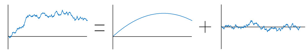 Figure 1
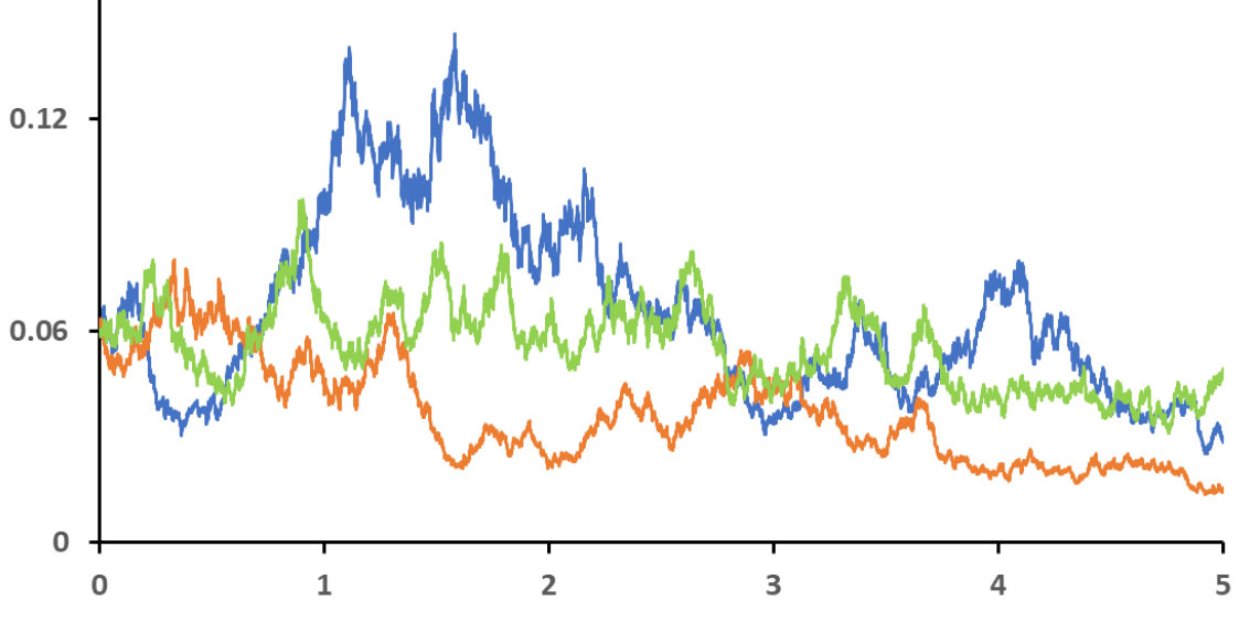 Figure 2
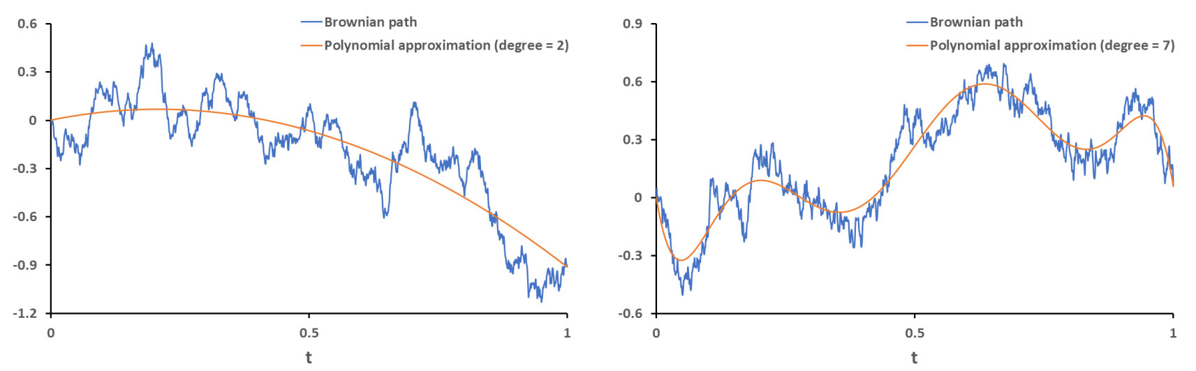 Figure 3
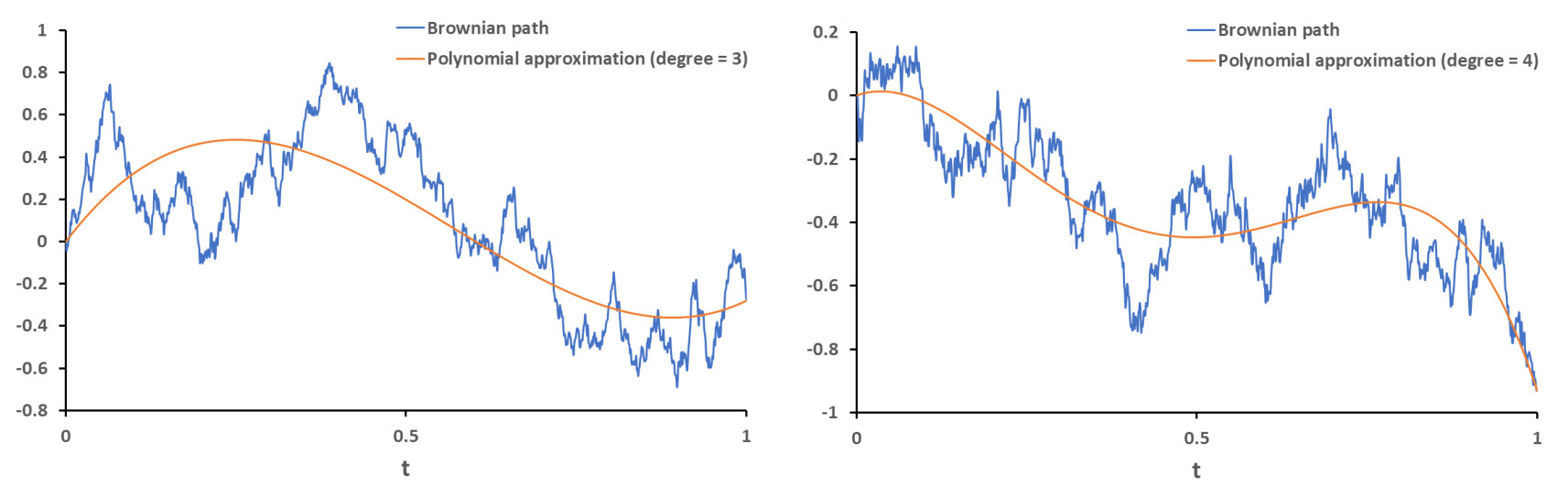 Figure 4
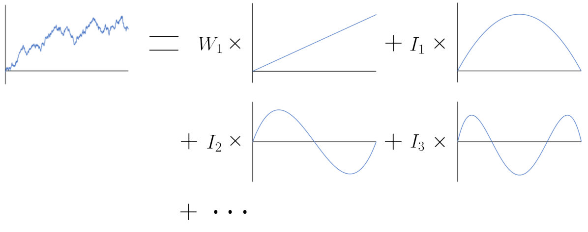 Figure 5
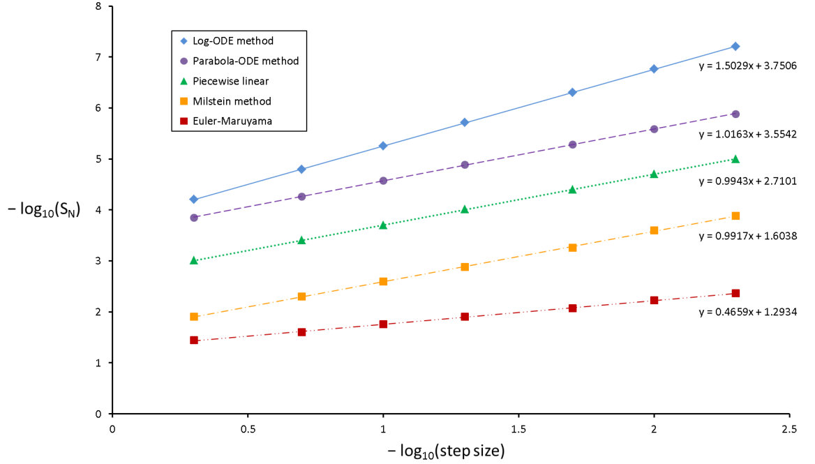 Figure 6
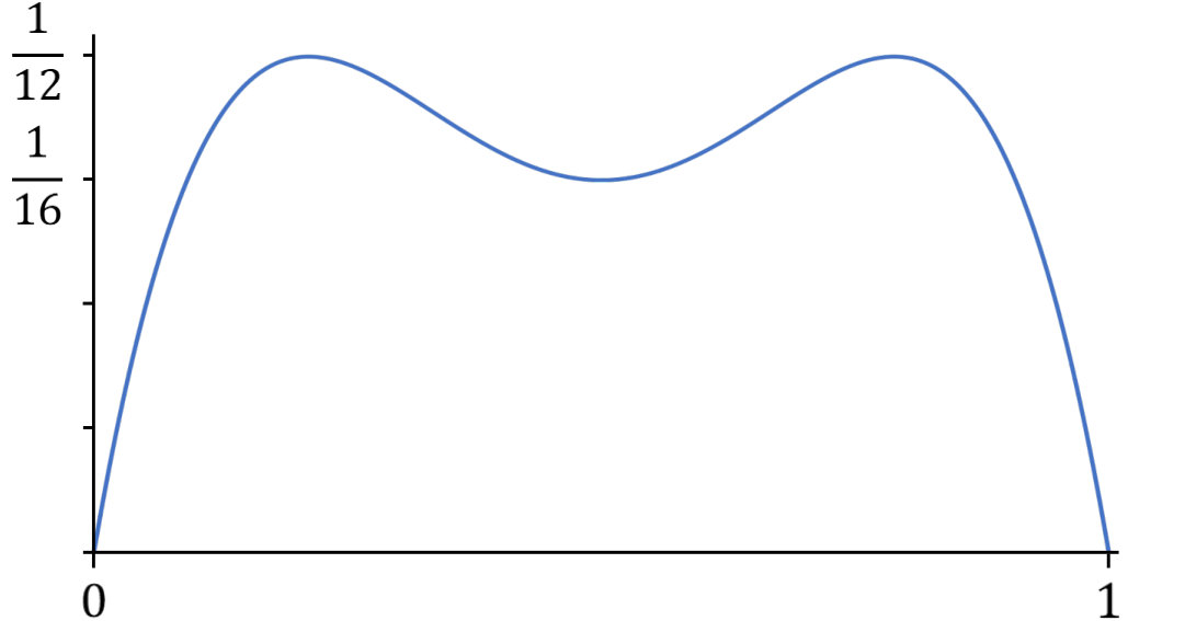 Figure 7
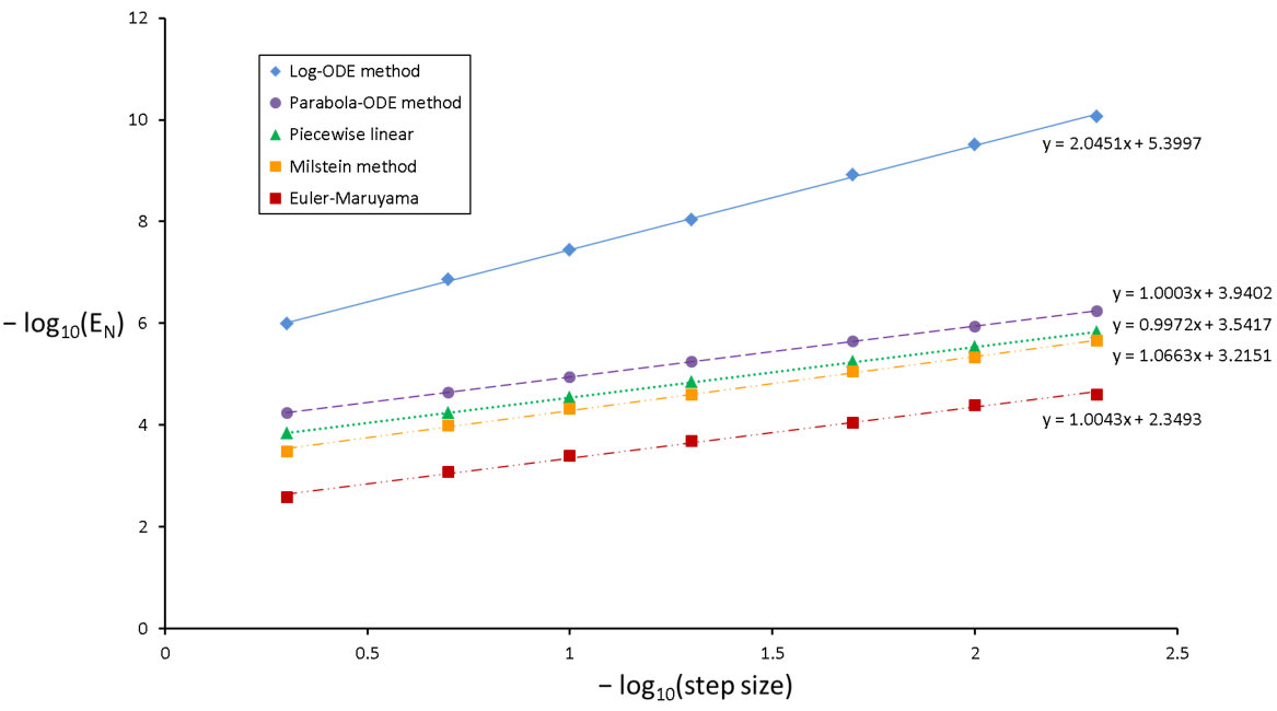 Figure 8
| Symbol | Meaning | Page |
| a standard real-valued Brownian motion. | 2 | |
| a standard real-valued Brownian bridge on . | 5 | |
| a Borel measure on defined by a singular weight function. | 5 | |
| for all open intervals . | ||
| a family of Jacobi-like polynomials with that are orthogonal with respect to weight function | 5 | |
| a time integral of times the polynomial over , | 5 | |
| the covariance function of , that is . | 5 | |
| the -th order -Jacobi polynomial on . | 11 | |
| the -th order Legendre polynomial on , i.e. . | 13 | |
| a solution of the Stratonovich SDE on the finite interval , | 14 | |
| where , and denote smooth vector fields. | ||
| (Itô SDEs will be defined on fixed intervals with the same form) | ||
| a general closed subinterval of , usually considered small. | 14 | |
| the step size that a numerical method uses, typically . | 14 | |
| the increment of Brownian motion over , . | 14 | |
| the Brownian parabola corresponding to over some interval. | 15 | |
| the Brownian arch corresponding to defined as . | 15 | |
| the rescaled space-time Lévy area of Brownian motion on , | 15 | |
| the space-space-time Lévy area of Brownian motion over , | 17 | |
| an approximation for the true solution of a Stratonovich SDE. | 19 | |
| the standard Lie bracket of vector fields, . | 19 |
| Log-ODE | Parabola | Linear | Milstein | Euler | |
|---|---|---|---|---|---|
| Estimated time to achieve | 0.179 | 0.405 | 1.47 | 15.4 | 0.437 |
| an accuracy of | (s) | (s) | (s) | (s) | (days) |
| Estimated time to achieve | 0.827 | 3.90 | 14.9 | 157 | 61.2 |
| an accuracy of | (s) | (s) | (s) | (s) | (days) |
| Log-ODE | Parabola | Linear | Milstein | Euler | |
| Computation time (s) | 2.44 | 2.95 | 1.48 | 1.18 | 1.17 |
| Log-ODE | Parabola | Linear | Milstein | Euler | |
|---|---|---|---|---|---|
| Estimated time to achieve | 0.240 | 1.69 | 2.15 | 2.78 | 25.5 |
| an accuracy of | (s) | (s) | (s) | (s) | (s) |
| Estimated time to achieve | 0.240 | 16.9 | 21.6 | 24.1 | 252 |
| an accuracy of | (s) | (s) | (s) | (s) | (s) |
Peer Reviews
No public reviews on file for this paper yet. If you reviewed it on a platform where reviews are public (OpenReview, ICLR, NeurIPS, ICML), you can paste yours below so the community can read it here.
Code & Models
Videos
No videos yet. Explain this paper in a talk, walkthrough, or lecture? Add one.
An optimal polynomial approximation of
Brownian motion
James Foster††Mathematical Institute, University of Oxford, Woodstock Road, Oxford, OX2 6GG, UK.
[email protected], [email protected], [email protected]. Research supported by the Engineering and Physical Sciences Research Council [EP/N509711/1].
Terry Lyons Supported by the EPSRC grant DATASIG, Alan Turing Institute and Oxford-Man Institute.
Harald Oberhauser††footnotemark:
Abstract
In this paper, we will present a strong (or pathwise) approximation of standard Brownian motion by a class of orthogonal polynomials. The coefficients that are obtained from the expansion of Brownian motion in this polynomial basis are independent Gaussian random variables. Therefore it is practical (requires independent Gaussian coefficients) to generate an approximate sample path of Brownian motion that respects integration of polynomials with degree less than . Moreover, since these orthogonal polynomials appear naturally as eigenfunctions of the Brownian bridge covariance function, the proposed approximation is optimal in a certain weighted sense.
In addition, discretizing Brownian paths as piecewise parabolas gives a locally higher order numerical method for stochastic differential equations (SDEs) when compared to the piecewise linear approach. We shall demonstrate these ideas by simulating Inhomogeneous Geometric Brownian Motion (IGBM). This numerical example will also illustrate the deficiencies of the piecewise parabola approximation when compared to a new version of the asymptotically efficient log-ODE (or Castell-Gaines) method.
keywords:
Brownian motion, polynomial approximation, numerical methods for SDEs
AMS:
41A10, 60J65, 60L90, 65C30
1 Introduction
Brownian motion is a central object for modelling real-world systems that evolve under the influence of random perturbations [1]. In applications where methods discretize Brownian motion, usually only increments of the path are generated [2]. In this setting, the best approximation of Brownian motion that is measurable with respect to these increments is given by the piecewise linear path that agrees on discretization points [3]. This motivates the following natural question: Are there better discrete approximations of Brownian motion than piecewise linear? The next simplest approximant would be a piecewise polynomial, though it is not clear whether this would be advantageous for tackling problems such as SDE simulation. This paper can be viewed as a logical continuation of [4], where a polynomial wavelet representation of Brownian motion was proposed. These wavelets were constructed to capture certain “geometrical features” of the path, namely the integrals of the Brownian motion against monomials. We shall investigate the practical applications of these polynomials and their geometrical features in the numerical analysis of SDEs.
The paper is organised as follows. In Section 2, we shall state and prove the main result of the paper (Theorem 5). This will be a Karhunen-Loève theorem for the Brownian bridge, where the orthogonal functions used in the approximation are polynomials. Furthermore, we shall explicitly show that each basis function is proportional to a shifted -Jacobi polynomial but with the nonstandard exponents . This enables us to construct these orthogonal polynomials using recurrence relations, or as the difference of two shifted Legendre polynomials whose degrees differ by two. The resulting polynomial expansion of Brownian motion was independently discovered by Habermann in [5], where a sharp convergence rate of O\big{(}\frac{1}{\sqrt{n}}\big{)} is established111A Matlab demonstration can be found at chebfun.org/examples/stats/RandomPolynomials.html. In Section 3, we shall investigate some significant consequences of the main theorem.
Theorem 1**.**
Let denote a standard real-valued Brownian motion on . Let be the unique -th degree random polynomial with a root at [math] and satisfying
[TABLE]
Then , where is a centered Gaussian process independent of .
The above theorem has a simple yet striking conclusion, namely that polynomials can be unbiased approximants of Brownian motion. In addition, the first non-trivial case () already has interesting applications within the numerical analysis of SDEs. One reason is that parabolas can capture the “ space-time area” of Brownian motion.
Therefore discretizing Brownian motion using a piecewise parabola gives a locally high order methodology for numerically solving one-dimensional SDEs. However, since certain triple iterated integrals of Brownian motion and time are partially matched by these parabolas, we expect this method to have only an rate of convergence (where denotes the step size used). This gives motivation for the following theorem:
Theorem 2**.**
Let be the (unique) quadratic polynomial with a root at [math] and
[TABLE]
Then the following third order iterated integral of Brownian motion can be estimated:
[TABLE]
The above theorem can be directly incorporated into the stochastic Taylor method as well as the log-ODE or Castell-Gaines method (see [6], [7]). We will show that by estimating this non-trivial iterated integral with its conditional expectation, we can design numerical methods that enjoy high orders of both strong and weak convergence. Specifically, for a general SDE that is driven by a one-dimensional Brownian motion and governed by sufficiently regular vector fields (smooth with bounded derivatives), the numerical methods that correctly utilize the above conditional expectation will have a strong convergence rate of as well as a weak convergence rate of .
These high orders of convergence can also be achieved in the multidimensional setting provided the vector fields governing the SDE satisfy certain commutativity conditions. For example, this estimator has applications for simulating SDEs with additive noise:
[TABLE]
where is a smooth vector field on , is constant and is now -dimensional. By considering Theorem 2, we expect that is well approximated (for small ) by
[TABLE]
where denotes the solution of the below ODE driven by a “ Brownian parabola” ,
[TABLE]
This parabola-driven ODE can then be discretized using a three-stage Runge-Kutta method and the resulting SDE approximation shall be investigated in a future work.
Since these methods are based on the conditional expectation given by Theorem 2, they are designed to minimize the leading error term within local Taylor expansions. This sense of optimality is conceptually similar to that of the asymptotically efficient SDE approximations developed by Clark [8], Newton [9, 10] and Castell & Gaines [6]. The key difference is that we are employing additional integral information about . Hence, this line of research could provide a further insight into the approximation of Itô integrals using linear path information, where there already are a number of results concerning the computational complexity of methods (see [11], [12] and [13]).
Most notably, Tang and Xiao [11] consider the same triple iterated integral as in (2) and present an asymptotically optimal approximation that performs well when a limited number of random variables are used (see Table 2 for these numerical results). Whilst there are other senses of optimality (such as those discussed in [14] and [15]) that could be used when analysing the proposed approximations of Brownian motion and SDE solutions, we shall estimate errors in an sense throughout the paper. In particular, we can apply the main result to quantify the error of the new estimator.
Theorem 3**.**
Using the same notation as before, we have the following variance:
[TABLE]
In Section 4, we demonstrate the applicability of these ideas to SDE simulation through various discretizations of Inhomogeneous Geometric Brownian Motion (IGBM)
[TABLE]
where and are the mean reversion parameters and is the volatility.
In mathematical finance, IGBM is an example of a short rate model that can be both mean-reverting and non-negative. It is therefore suitable for modelling interest rates, stochastic volatilities and default intensities [16]. From a mathematical viewpoint, IGBM is one of the simplest SDEs that has no known method of exact simulation [17]. By incorporating the ideas provided by the main theorem into the log-ODE method, we will produce a state-of-the-art numerical approximation of IGBM. Although the vector fields for IGBM are not bounded, our numerical evidence indicates that the method has a strong convergence rate of and a weak convergence rate of .
1.1 Notation
Below is some of the notation that is used throughout the paper.
2 Main result
It was shown in [4] that Brownian motion can be generated using Alpert-Rokhlin multiwavelets (see [18]). The mother functions that generate this wavelet basis are supported on and are defined using polynomials as follows:
Definition 4** (Alpert-Rokhlin wavelets).**
For , define the functions as piecewise polynomials of degree with pieces on , that satisfy the following conditions for all and
[TABLE]
The Alpert-Rokhlin multiwavelets of order can now be generated by translating and scaling the mother functions .
[TABLE]
for and .
Whilst our results will not be presented in terms of the above wavelets, we shall see that the polynomials of interest are directly related to conditions (3), (4) and (5). The main result of this paper gives an effective method for approximating sample paths of Brownian motion by a class of Jacobi-like polynomials. The proof is based on the interpretation of these polynomials as eigenfunctions of an integral operator defined by the Brownian bridge covariance function222The Brownian bridge is the centered Gaussian process with covariance .. These orthogonal polynomials, which lie at the heart of this paper, will also help us interpret the geometrical features that certain normally distributed iterated integrals encode about the Brownian path.
Theorem 5** (A polynomial Karhunen-Loève theorem for the Brownian bridge).**
Let denote a Brownian bridge on and consider the Borel measure given by
[TABLE]
Then there exists a family of orthogonal polynomials with and
[TABLE]
with denoting the Kronecker delta, such that admits the following representation
[TABLE]
where is the collection of independent centered Gaussian random variables with
[TABLE]
and
[TABLE]
Furthermore, is an optimal orthonormal basis of for approximating by truncated series expansions with respect to the following weighted norm
[TABLE]
where is a square -integrable process.
Proof.
Our argument is that of the Karhunen-Loève theorem in general spaces. Note that is a square -integrable process as
[TABLE]
Let denote the covariance function for the standard Brownian bridge on . Since , it can be shown by direct calculation that satisfies
[TABLE]
Hence, it follows that the integral operator given by
[TABLE]
is well-defined and continuous. In addition, the variance function for is -integrable as
[TABLE]
Therefore, we can apply Mercer’s theorem for kernels on general spaces (see [19]). It then follows from Mercer’s theorem that there exists an orthonormal set of consisting of eigenfunctions of such that the corresponding sequence of eigenvalues is non-negative. Moreover, the eigenfunctions corresponding to non-zero eigenvalues are continuous on and the kernel has the representation
[TABLE]
where the series (8) converges absolutely and uniformly on compact subsets of .
In the next part of the proof, we will see that each is a polynomial of degree . As each is an eigenfunction of , we have
[TABLE]
Since , it follows that and for each . Therefore by using the Leibniz integral rule to twice differentiate both sides of (9) and then multiplying by , we observe that satisfies the differential equation
[TABLE]
Since , we have that . Differentiating the LHS of the ODE (10) produces
[TABLE]
For , we define the function
[TABLE]
Thus satisfies the following differential equation
[TABLE]
Remarkably, this is the Legendre differential equation [20]. It then follows using classical Sturm-Liouville theory that and is proportional to the -th Legendre polynomial. Therefore, the derivative will be a constant multiple of the -th shifted Legendre polynomial and hence each is a polynomial of degree .
We can now define the following integrals for ,
[TABLE]
It follows from Fubini’s theorem that
[TABLE]
Since each is defined by a linear functional on the same Gaussian process , we see from the above that is a collection of uncorrelated (and therefore independent) Gaussian random variables with
[TABLE]
Finally, the convergence we require follows as
[TABLE]
which converges to [math] by Mercer’s theorem (8).
All that remains is to prove optimality for the truncated series expansions of (6). Let denote an orthonormal basis of such that
[TABLE]
For , we consider an error process associated with the above: .
Then the square norm of the -th error process admits the following expansion,
[TABLE]
Integrating the above with respect to and using the orthogonality of gives
[TABLE]
Note that any optimal orthonormal basis of solves the following problem:
[TABLE]
By introducing Lagrange multipliers , we wish to find functions that minimize
[TABLE]
We will now consider the following square integrable functions, defined for :
[TABLE]
Therefore it is enough to find a family of functions in which minimizes
[TABLE]
To find a minimizer, we set the functional derivative of with respect to to zero.
[TABLE]
By using the definitions of and , it is trivial to show the above is equivalent to
[TABLE]
which is satisfied if and only if are eigenfunctions of . ∎
This result can naturally be extended to express Brownian motion using polynomials.
Theorem 6**.**
If is a standard Brownian motion and is the associated bridge process on , then by Theorem 5, we have the below representation of :
[TABLE]
where for , and the random variables are independent of .
In the rest of this section, we shall study the key objects introduced in Theorem 5. Since each orthogonal polynomial lies in , it must have roots at [math] and . Therefore is itself a polynomial but with degree , and one can repeatedly apply the integration by parts formula to the stochastic integrals defined by (7). This enables us to express each in terms of iterated integrals of Brownian motion. Moreover, as has precisely non-zero derivatives, the highest order iterated integral that is required to fully describe is .
So by applying the integration by parts formula as above, we can construct a lower triangular matrix with non-zero diagonal entries that characterizes the relationship between and a set of iterated integrals of Brownian motion.
Hence, for , we can express the independent Gaussian integrals as
[TABLE]
Since is an invertible matrix, it follows that the column vectors appearing in (13) both encode the same information about the Brownian bridge. This enables us to establish a connection between Brownian motion, iterated integrals and polynomials.
Theorem 7**.**
Consider the below conditional expectation of Brownian motion,
[TABLE]
where . Then is the unique polynomial of degree with a root at [math] that matches the increment and iterated time integrals of the path given by:
[TABLE]
Proof.
It is a direct consequence of (13) that . Hence by (12) and independence of the random variables , we have that
[TABLE]
Thus is indeed a polynomial of degree with a root at [math] and that matches the increment of the Brownian path. Without loss of generality we can now assume . All that remains is to argue matches the iterated integrals given in (15). Using the orthogonality of , it follows directly from (16) that for :
[TABLE]
Hence matches the integrals of Brownian motion against polynomials with degree at most . By the same argument used in the derivation of (13), it follows that matches the various iterated time integrals given in the statement of the theorem. The uniqueness of is now a consequence of having different constraints. ∎
2.1 Properties of orthogonal polynomials
Although Theorem 5 and Theorem 6 are interesting results from a theoretical point of view, both lack an explicit construction of the polynomials that could be implemented in practice. On the other hand, it was shown that the defining eigenfunction property of each implies that its derivative is proportional to the -th shifted Legendre polynomial. Hence the family is the (normalized) shifted -Jacobi polynomials but with . Since Jacobi polynomials are typically studied with , it is necessary to show there exists a well-defined limit when the parameters approach .
Definition 8**.**
For , the -th degree -Jacobi polynomial is
[TABLE]
Naturally, for this definition to be unambiguous, we will require the following lemma.
Lemma 9**.**
Let denote the -th degree -Jacobi polynomial on . Then for , there exists a real-valued polynomial such that \big{\|}P_{k}-P_{k}^{(\alpha,\beta)}\big{\|}_{\infty}\rightarrow 0 as .
Proof.
Below is an identity for Jacobi polynomials, with , given in [21].
[TABLE]
Therefore, we shall define the -th degree polynomial over the interval by
[TABLE]
It is straightforward to verify that for . So by induction and the recurrence relation for Jacobi polynomials (see [21]), we have:
[TABLE]
for all . Hence by the dominated convergence theorem with (17) and (18), it follows that will converge pointwise to as for each . Finally, the result follows as and are always polynomials with degree . ∎
Using the above definition for -Jacobi polynomials, we can give an explicit formula for the orthonormal polynomials appearing in Theorems 5 and 6.
Theorem 10**.**
Suppose each has a positive leading coefficient. Then for ,
[TABLE]
Proof.
The following identity for -Jacobi polynomials is stated in [21]:
[TABLE]
for and . Applying the change of variables, , we have
[TABLE]
for and . By definition 8, taking the limit will yield
[TABLE]
Therefore by setting , we have
[TABLE]
Recall that is proportional to the -th shifted Legendre polynomial . Similarly, we saw in the proof of Lemma 9 that the derivative of is . As and are zero at their respective endpoints, we have that each must be proportional to . The result now follows from the above calculations. ∎
Having identified an explicit formula for the eigenfunctions in (19), we shall now describe two methodologies for computing the Jacobi-like polynomials \big{\{}P_{k}^{(\text{-}1,\text{-}1)}\big{\}}.
The first approach is to use the three-term recurrence relation in the theorem below.
Theorem 11** (Recurrence relation for -Jacobi polynomials).**
For ,
[TABLE]
where the initial polynomials are given by
[TABLE]
Proof.
The below recurrence relation for Jacobi polynomials is presented in [21],
[TABLE]
for and . By definition 8, it is possible to take the limit provided that . Therefore, taking this limit and setting produces
[TABLE]
for . Dividing the above by gives the required recurrence relation (20). Finally the below formula, stated in [21], can be used to compute and :
[TABLE]
As before we take in the above to obtain an explicit formula for . ∎
In addition to computing these polynomials via a recurrence relation, it is also possible to represent each as the difference of two (rescaled) Legendre polynomials. Since the Legendre polynomials already have efficient implementations in the majority of high-level programming languages, this second approach is particularly appealing.
Theorem 12** (Relationship between the Jacobi-like and Legendre polynomials).**
For , we have
[TABLE]
where denotes the -th degree Legendre polynomial defined on .
Proof.
Recall that \frac{d}{dx}\big{(}P^{(\text{-}1,\text{-}1)}_{n+1}\hskip 0.7113pt\big{)}=\frac{n}{2}P^{(0,0)}_{n} for , where is the -th degree Legendre polynomial. Therefore differentiating both sides of (20) yields
[TABLE]
Hence by simplifying and rearranging the above, we have that for ,
[TABLE]
We see the last term is zero by a recurrence relation for Legendre polynomials [20]. ∎
In addition to viewing the polynomials as orthogonal with respect to the weight function , we can characterize them via their iterated time integrals. In particular, for , it follows from the integration by parts formula that
[TABLE]
Hence for , is a polynomial with degree that has roots at [math] and as well as trivial iterated integrals against time. By additionally specifying the -th iterated time integral, it is then possible to characterize the -th polynomial .
To conclude this section, we will address the relationship between the orthogonal Jacobi-like polynomials and the Alpert-Rokhlin wavelets given in definition 4. Since each is proportional to the -th shifted Legendre polynomial, the family of polynomials is orthogonal with respect to the standard inner product. This orthogonality is exactly what is needed to satisfy the conditions (4) and (5). Hence for any there exists an Alpert-Rokhlin mother function of order that is a piecewise polynomial where both pieces can be rescaled and translated to give .
3 Applications to SDEs
Consider the Stratonovich SDE on the interval
[TABLE]
where and denote bounded vector fields on with bounded derivatives. It then follows from the standard Picard iteration argument that there exists a unique strong solution to (21). An important tool in the numerical analysis of this solution is the stochastic Taylor expansion (see chapter 5 of [22] for a comprehensive review). For the purposes of this paper, we only require the following specific Taylor expansion.
Theorem 13** (High order Stratonovich-Taylor expansion).**
Let denote the unique strong solution to (21) and let . Then can be expanded as follows:
[TABLE]
where and the remainder term has the following uniform estimate for ,
[TABLE]
where the constant depends only on the vector fields of the differential equation.
From a numerical perspective, the most challenging terms presented in (22) are those that involve non-trivial third order iterated integrals of Brownian motion and time. Moreover, the most significant source of discretization error that high order numerical methods will experience is generally due to approximating these stochastic integrals. By representing Brownian motion as a (random) polynomial plus independent noise, we shall derive a new optimal and unbiased estimator for these third order integrals.
Theorem 14**.**
Let denote a standard real-valued Brownian motion on . Let be the unique -th degree random polynomial with a root at [math] and satisfying
[TABLE]
Then , where is a centered Gaussian process independent of .
Furthermore, has the following covariance function:
[TABLE]
where denotes the standard Brownian bridge covariance function and , are the eigenvalues and eigenfunctions that were defined in the proof of Theorem 5.
Proof.
It follows from the integration by parts formula that matches the increment and iterated time integrals of Brownian motion that appear in (15). Hence is also the polynomial defined in Theorem 7 and where
[TABLE]
Then by Theorem 5, is a centered Gaussian process that is independent of . In addition, the covariance function defining can be directly computed as follows:
[TABLE]
Note that the final line is achieved using the representation of given by (8). ∎
The above theorem has an interesting conclusion, namely that there exist unbiased polynomial approximants of Brownian motion for which the error process can be independently estimated in an sense. In particular, this theorem already has numerical applications in the case when and motivates the following definitions:
Definition 15**.**
The standard Brownian parabola is the unique quadratic polynomial on with a root at [math] and satisfying
[TABLE]
Definition 16**.**
The standard Brownian arch is the process . By Theorem 14, is the centered Gaussian process on with covariance function
[TABLE]
Definition 17**.**
The rescaled space-time Lévy area of Brownian motion over an interval with length encodes the signed area of the associated bridge process,
[TABLE]
Remark 3.18**.**
Since , we have that corresponds to as defined in Theorem 5. Thus, and is independent of .
By applying the natural scaling of Brownian motion, one can define the Brownian parabola and Brownian arch processes over any interval with finite size . Whilst the Brownian arch can be viewed in a similar light to the Brownian bridge, there are clear qualitative and quantitative differences in their covariance functions. In particular, the Brownian arch has less variance at its midpoint compared to most points in \big{(}by which we mean that |\{u\in[s,t]:\operatorname{Var}(Z_{u})\leq\operatorname{Var}(Z_{\frac{1}{2}(s+t)})\}|<\frac{1}{2}h\big{)}. This is in contrast to the Brownian bridge, which has most variance at its midpoint. In fact, the Brownian parabola gives a relatively uniform estimate of the original path.
Using these new definitions, we can study the high order integrals appearing in (22).
Theorem 3.19** (Conditional expectation of a non-trivial Brownian time integral).**
[TABLE]
Proof 3.20**.**
By the natural Brownian scaling it is enough to prove the result on . Recall that where the parabola is completely determined by and is independent of . This leads to a decomposition for the LHS of (24).
[TABLE]
The result now follows by evaluating the above integrals.
The above theorem has practical applications for SDE simulation as and are independent Gaussian random variables and can be easily generated or approximated. That said, we should first discuss how the iterated integrals within (22) are connected.
Definition 3.21**.**
The space-space-time Lévy area of Brownian motion over an interval is defined as
[TABLE]
We can interpret as an area between the processes and . Moreover, rough path theory provides an algebraic structure (called the log-signature) that relates to the iterated integrals of space-time Brownian motion and ultimately to SDE solutions via the log-ODE method (see [23] for an overview). For our purposes, it is enough to give formulae relating these Lévy areas to integrals.
Theorem 3.22**.**
Let and denote the Lévy areas of Brownian motion given by definitions 17 and 3.21 respectively. Then the following integral relationships hold,
[TABLE]
Proof 3.23**.**
The result follows from numerous applications of integration by parts.
We can now present the new unbiased estimator for third order iterated integrals of Brownian motion and time. The proposed estimator is fast to compute and the best approximation of these integrals that is measurable with respect to .
Theorem 3.24** (Conditional moments of Brownian space-space-time Lévy area).**
[TABLE]
Proof 3.25**.**
The expectation (25) is simply a consequence of Theorems 3.19 and 3.22. Without loss of generality, we will consider the above conditional variance on . Since is determined using the increment and space-time Lévy area , we have
[TABLE]
Recall where are independent centered Gaussian random variables.
In particular, this means that and have the same law. Therefore, we have that
[TABLE]
[TABLE]
The remaining two terms were resolved with assistance from Wolfram Mathematica.
[TABLE]
[TABLE]
By Theorem 3.22, the above gives an explicit formula for the conditional variance (26).
[TABLE]
By the natural Brownian scaling, the result on the interval directly follows.
Remark 3.26**.**
The conditional variance (26) allows one to estimate local errors for certain numerical methods and thus may be useful when choosing step sizes.
Therefore in order to propagate a numerical solution of (21) over an interval , one can generate exactly and then approximate using Theorem 3.24. However, there are many numerical methods that could be used to solve a given SDE.
3.1 Examples of ODE methods
We will consider the following two methods:
Definition 3.27** (High order log-ODE method).**
For a fixed number of steps we can construct a numerical solution of (21) by setting and for each , defining to be the solution at of the following ODE:
[TABLE]
where , and denotes the standard Lie bracket of vector fields.
Definition 3.28** (The parabola-ODE method).**
For a fixed number of steps we can construct a numerical solution of (21) by setting and for each , defining to be the solution at of the following ODE:
[TABLE]
where and .
In both numerical methods the true solution at time can be approximated by . Whilst there are different ways of interpolating between the successive approximations and , for this paper we will simply interpolate between such points linearly. To analyse the above methods, we shall first note the key differences between them. The first important distinction between the two methods is a purely practical one. Although both of these methods involve computing a numerical solution of an ODE, the parabola method does not require one to explicitly resolve vector field derivatives. The second significant difference can be seen in the Taylor expansions of the methods.
Theorem 3.29**.**
Let be the one-step approximation defined by the log-ODE method on the interval with initial value . Then for sufficiently small
[TABLE]
Similarly, let denote the one-step approximation given by the parabola-ODE method on the interval with the same initial value. Then for sufficiently small
[TABLE]
Note that denotes terms which can be estimated in an sense as in (23).
Proof 3.30**.**
In order to derive (29), we must compute the Taylor expansion of (27). Let denote the vector field defined in (27) that was constructed from and . Then is smooth, and it follows from the classical Taylor’s theorem for ODEs that
[TABLE]
We shall first consider the remainder term, which can be directly estimated as follows:
[TABLE]
*One can define the degree of each term in the above Taylor expansion by counting the number of times functions from appear. Therefore, after expanding the fifth derivative of we can see that the remainder term has a degree of five. Since the largest component of is , both and its derivatives are . Hence the remainder term in the above Taylor expansion will be as in (23). Moreover, the only terms of degree four that are not are those involving .
It is now enough to analyse just the terms appearing in the first line of the expansion. By substituting the formula for given by (27) into the first line and then rearranging the resulting terms, we can obtain a Taylor expansion for that resembles (22) as*
[TABLE]
[TABLE]
Therefore, by summing the above formulae for (and its derivatives) we can derive an expansion of in terms of and \big{(}h,W_{s,t},H_{s,t}\big{)} that has an O\big{(}h^{\frac{5}{2}}\big{)} remainder. By comparing this with the stochastic Taylor expansion (22), the result (29) follows.
Arguing (30) is fairly straightforward and does not require extensive computations. Using the substitution for , the ODE (28) can be rewritten as
[TABLE]
where denotes the Brownian parabola defined by on the interval .
By emulating the derivation of the Stratonovich-Taylor expansion (22), it is possible to Taylor expand (31) in the same fashion. The only difference is that Stratonovich integrals with respect to are replaced with Riemann-Stieltjes integrals against .
In particular, by the change-of-variable formula for ODEs (exercise 3.17) given in **[24]**, we see that the remainder term of such a Taylor expansion will have the below form:
[TABLE]
where we have identified an additional “ zero” coordinate of with time, , and for each index , the function consists of finitely many compositions of along with their derivatives (and thus is Lipschitz continuous).
Therefore each term in the expansion of (31) can be estimated in by applying the natural Brownian scaling to the corresponding iterated integral of with time. As before, the largest differences are the terms involving third order integrals. Fortunately, iterated integrals of the Brownian parabola can be computed explicitly:
[TABLE]
The result (30) is now a direct consequence of Theorem 3.22 along with the above.
Theorem 3.29 shows that both methods give a one-step approximation error of . This means that the log-ODE and parabola-ODE methods are both locally high order; however there is a significant difference in how these methods propagate local errors. The reason is that the components of the log-ODE local errors give a martingale, whilst the part for each parabola-ODE local error has non-zero expectation. Thus the log-ODE method is globally high order whilst the parabola method is not. However, since the parabola-ODE method is straightforward to implement and locally high order, one could expect it to perform well compared to other low order methods. In the numerical example, we shall see that the parabola method has the same order of convergence as the piecewise linear approach but gives significantly smaller errors. To conclude this section, we will present the orders of convergence for both methods.
Definition 3.31** (Strong convergence).**
A numerical solution for (21) is said to converge in a strong sense with order if there exists a constant such that
[TABLE]
for all sufficiently small step sizes .
Definition 3.32** (Weak convergence).**
A numerical solution for (21) is said to converge in a weak sense with order if for any polynomial there exists such that
[TABLE]
for all sufficiently small step sizes .
Theorem 3.33** (Orders of convergence).**
For a general SDE (21), the log-ODE method converges in a strong sense with order 1.5 and a weak sense with order 2.0. The parabola-ODE method converges in both a strong and weak sense with order 1.0.
Proof 3.34**.**
Note that Theorem 3.29 establishes the Taylor expansions of both methods. The strong convergence can then be shown as in the proof of Theorem 11.5.1 in [22]. Moreover, the proof of Theorem 11.5.1 also provides the orders of strong convergence. Similarly weak convergence follows directly from the Taylor expansions (29) & (30), and the rate of convergence can be shown as in the proof of Theorem 14.5.2 in [22].
4 A numerical example
We shall demonstrate the ideas presented so far using various discretizations of Inhomogeneous Geometric Brownian Motion (IGBM)
[TABLE]
where and are the mean reversion parameters and is the volatility. As the vector fields are smooth, the SDE (32) can be expressed in Stratonovich form:
[TABLE]
where and denote the “adjusted” mean reversion parameters.
IGBM is an example of a one-factor short rate model and has seen recent attention in the mathematical finance literature as an alternative to popular models [16, 17]. IGBM is also one of the simplest SDEs that has no known method of exact simulation. We will investigate the strong and weak convergence rates of the following methods:
Log-ODE method (see definition 3.27)
Since the vector fields of (33) give constant Lie brackets, this method becomes
[TABLE] 2. 2.
Parabola-ODE method (see definition 3.28)
As the SDE (33) is quite analytically tractable, this method is expressible as
[TABLE]
The integral above will be computed by -point Gauss-Legendre quadrature. 3. 3.
Piecewise linear method (see [25] for definition and proof of convergence)
Just as above, this method can be simplified to give a straightforward formula.
[TABLE] 4. 4.
Milstein method (see section 6 of [2] and section 10.3 of [22] for overviews)
For this method, we shall take the positive part to guarantee non-negativity.
[TABLE] 5. 5.
Euler-Maruyama method (see sections 4, 5 of [2] and section 10.2 of [22])
Just as above, we take the positive part of each step to ensure non-negativity.
[TABLE]
Note that the explicit formula for the log-ODE method comes from the Lie brackets:
[TABLE]
and the formula for the parabola-ODE method was derived using a change of variable.
The Euler-Maruyama and Milstein methods are included in the numerical experiment as benchmarks to test how the proposed methods compare to well-known methods. As before, we will be discretizing the SDE over a uniform partition with mesh size .
Below is the definition of the error estimators used to analyse the numerical methods.
Definition 4.35** (Strong and weak error estimators).**
For each , let denote a numerical solution of (32) computed at time using a fixed step size . We can define the following estimators for quantifying strong and weak convergence:
[TABLE]
where the above expectations are approximated by standard Monte-Carlo simulation and is the numerical solution of (32) obtained at time using the log-ODE method with a “ fine” step size of . The fine step size is chosen so that the error between and the true solution is negligible compared to . Note that and are both computed with respect to the same Brownian paths.
In this numerical example, we shall use the same parameter values as in [16], namely , , and . We will also fix the time horizon at .
We will now present our results for the numerical experiment that is described above. (Code for this example can be found at github.com/james-m-foster/igbm-simulation)
From the above graph we see that the log-ODE method is by far the most accurate. This is epitomized by the fact that the numerical error produced by steps of the log-ODE method is comparable to the error of the parabola method with steps. In addition, whilst there are three methods that share the same order of convergence it is evident there are magnitudes of difference between their respective accuracies. For example, the parabola method is seven times more accurate than piecewise linear. As one might expect, the Euler-Maruyama and Milstein schemes both perform poorly.
Nevertheless, in order to truly measure the performance of these numerical methods, we should consider the computational costs required for achieving a specified accuracy.
The above graph demonstrates that the log-ODE method is especially well-suited for weak approximation as it achieves a second order convergence rate in this example. Surprisingly, the middle three methods exhibit almost identical convergence profiles. As before, we can estimate the computational time needed to achieve given accuracies.
We expect the log-ODE and parabola methods to have about twice the computational cost as the other methods because each step requires generating two random variables. Table 3 confirms this and thus sampling may be a bottleneck for these methods. So overall, the numerical evidence supports our claim that the high order log-ODE method is currently a state-of-the-art method for the pathwise discretization of IGBM.
5 Conclusion
There are primarily three new results established in this paper:
An efficient strong polynomial approximation of Brownian motion
The main result allows one to construct a “smoother” Brownian motion as a finite sum of -Jacobi polynomials with independent Gaussian weights. Moreover, it was shown that the approximation is optimal in a weighted sense and the surrounding noise is an independent centered Gaussian process.
Unbiased approximation of third order Brownian iterated integrals
Iterated integrals of Brownian motion and time are important objects in the study of SDEs as they appear naturally within stochastic Taylor expansions. We have derived the -optimal estimator for a class of such integrals that is measurable with respect to the path’s increment and space-time Lévy area.
Simulation of Inhomogeneous Geometric Brownian Motion (IGBM)
IGBM is a mean-reverting short rate model used in mathematical finance and also one of the simplest SDEs that has no known method of exact simulation.
By incorporating the new iterated integral estimator into the log-ODE method we have developed a high order state-of-the-art numerical method for IGBM.
Furthermore, the results of this paper naturally lead to the following open questions:
Which weight functions give “ explicit eigenfunctions” for Brownian motion? (For example, we could try or with )
Is it possible to generalize the main theorem to fractional Brownian motion?
What are the most efficient Runge-Kutta methods for general one-dimensional SDEs that correctly use the new estimator for third order iterated integrals?
Is this polynomial expansion optimal for approximating Lévy area? (see [13])
Which conditional moments can be computed for a given stochastic integral?
How might we construct a piecewise linear path with the below properties?
[TABLE]
Would this method of construction lead to effective cubature paths? (see [26])
Given such a path, we can approximate (21) with a “ piecewise linear” ODE.
[TABLE]
(Along each piece of , we would discretize (36) using an appropriate solver)
How effective is the above piecewise linear ODE method for simulating SDEs?
Can we extend the approximations given in this paper to the SPDE setting?
The reference list from the paper itself. Each links out to its DOI / PubMed record.
- 1[1] R. M. Mazo , Brownian Motion: Fluctuations, Dynamics and Applications , Clarendron Press, Oxford, 2002.
- 2[2] D. J. Higham , An algorithmic introduction to numerical simulation of stochastic differential equations , SIAM Review, Volume 43, 2001.
- 3[3] J. M. C. Clark and R. J. Cameron , The maximum rate of convergence of discrete approximations for stochastic differential equations , Stochastic Differential Systems Filtering and Control, Volume 25 in Lecture Notes in Control and Information Sciences, Springer, 1980.
- 4[4] D. S. Grebenkov, D. Belyaev and P. W. Jones , A multiscale guide to Brownian motion , Journal of Physics A, Volume 49, 2015.
- 5[5] K. Habermann , A semicircle law and decorrelation phenomena for iterated Kolmogorov loops , https://arxiv.org/abs/1904.11484 , 2019.
- 6[6] F. Castell and J. G. Gaines , The ordinary differential equation approach to asymptotically efficient schemes for solution of stochastic differential equations , Annales de l’Institut Henri Poincaré, Volume 32, 1996.
- 7[7] S. J. A. Malham and A. Wiese , Stochastic Lie group integrators , Siam Journal on Scientific Computing, Volume 30, 2008.
- 8[8] J. M. C. Clark , An efficient approximation for a class of stochastic differential equations , Advances in Filtering and Optimal Stochastic Control, Proceedings of the IFIP-WG 7/1 Working Conference. Cocoyoc, Mexico, 1982. Lecture Notes in Control and Information Sciences, Volume 42, Berlin, 1982.
