Chebyshev Hierarchical Equations of Motion for Systems with Arbitrary Spectral Densities and Temperatures
Hasan Rahman, Ulrich Kleinekathoefer

TL;DR
This paper introduces a novel Chebyshev polynomial-based hierarchical equations of motion method for open quantum systems, capable of handling complex spectral densities and low temperatures more efficiently than traditional exponential schemes.
Contribution
It develops an alternative hierarchical equations of motion approach using Chebyshev polynomials and Bessel functions, extending applicability to arbitrary spectral densities and temperatures.
Findings
Effective for complex spectral densities and low temperatures
Comparable accuracy to benchmark calculations for zero-temperature noise
Discusses advantages and limitations of the Chebyshev-based scheme
Abstract
The time evolution in open quantum systems, such as a molecular aggregate in contact with a thermal bath, still poses a complex and challenging problem. The influence of the thermal noise can be treated using a plethora of schemes, several of which decompose the corresponding correlation functions in terms of weighted sums of exponential functions. One such scheme is based on the hierarchical equations of motion (HEOM), which is built using only certain forms of bath correlation functions. In the case where the environment is described by a complex spectral density or is at a very low temperature, approaches utilizing the exponential decomposition become very inefficient. Here we utilize an alternative decomposition scheme for the bath correlation function based on Chebyshev polynomials and Bessel functions to derive a hierarchical equations of motion approach up to an arbitrary order…
Click any figure to enlarge with its caption.
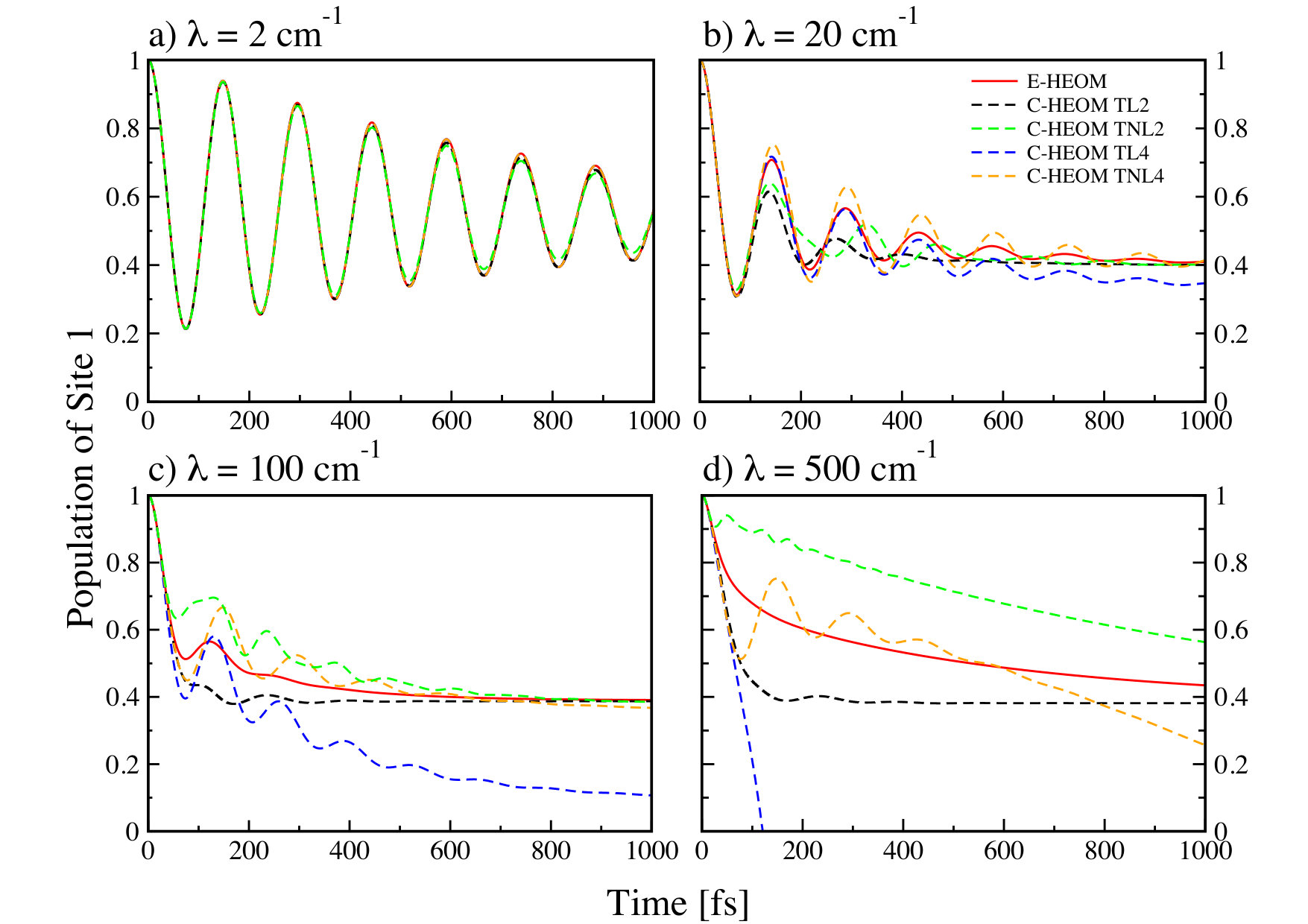 Figure 1
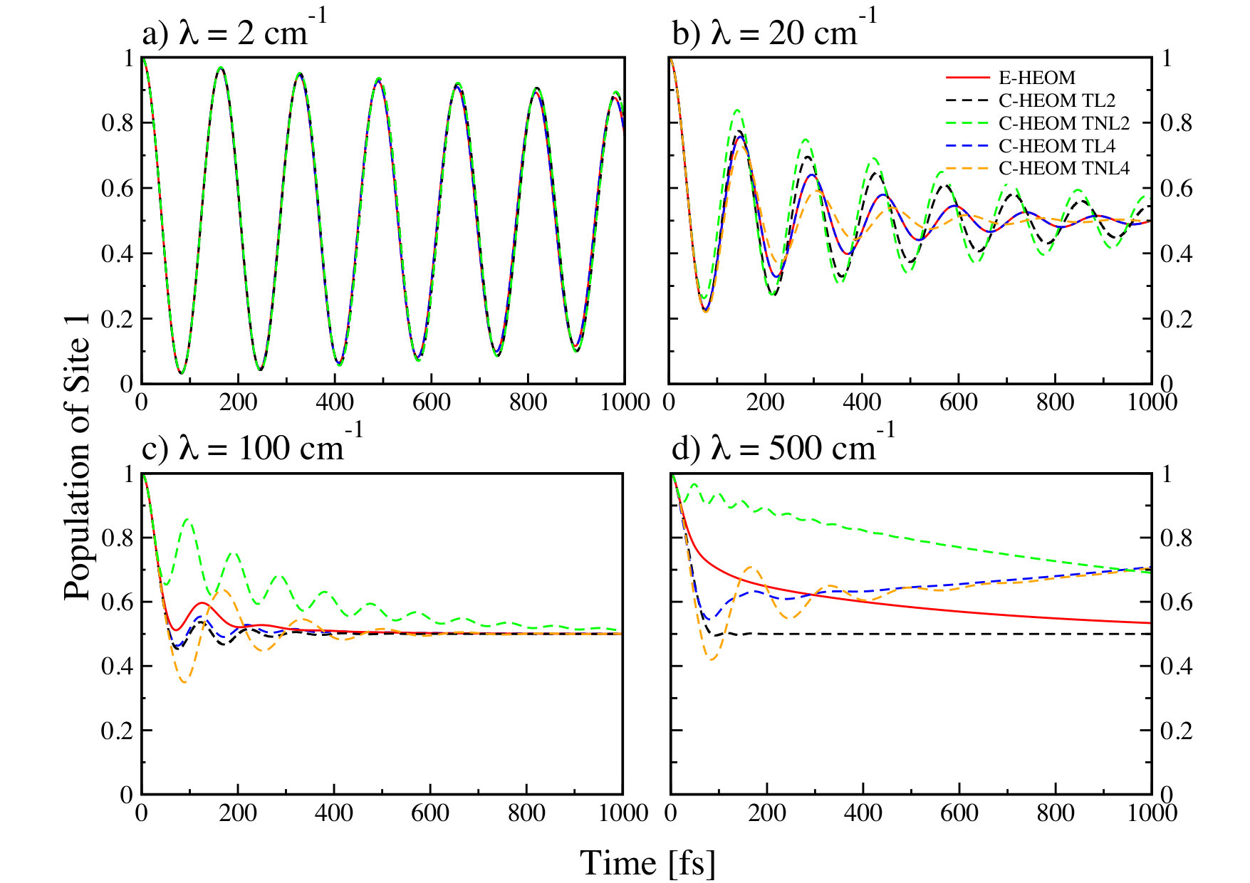 Figure 2
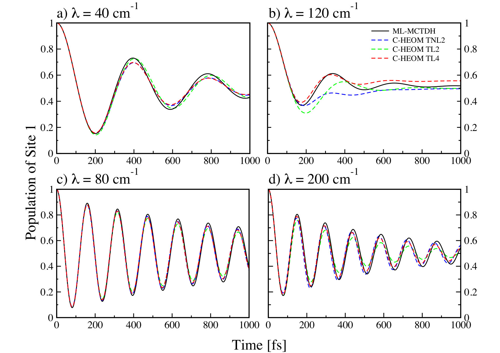 Figure 3
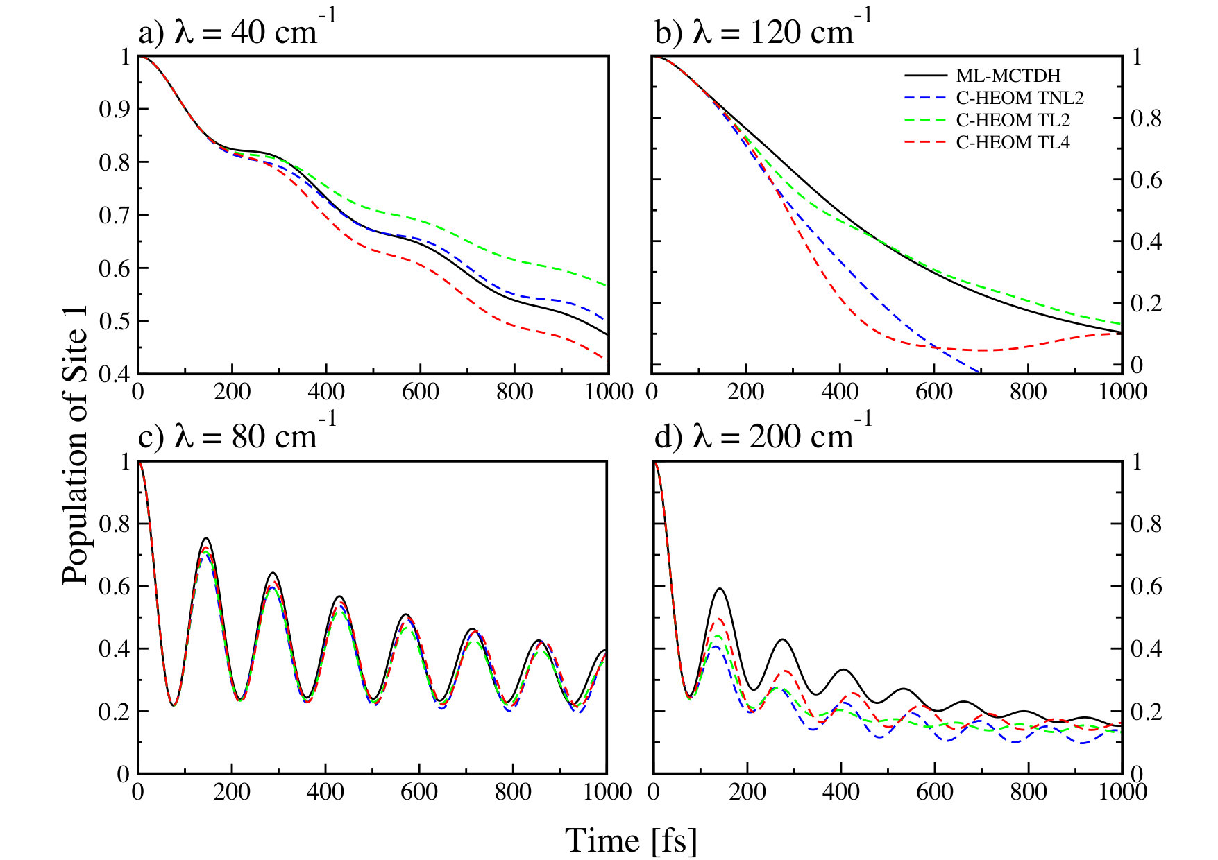 Figure 4
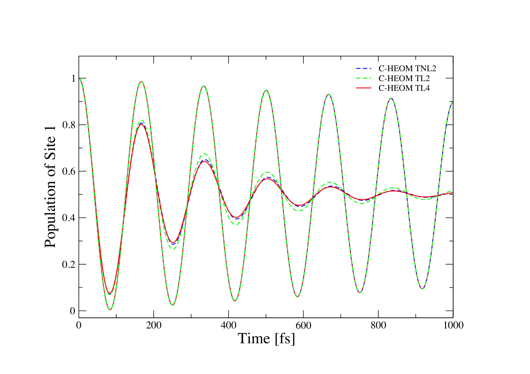 Figure 5
Peer Reviews
No public reviews on file for this paper yet. If you reviewed it on a platform where reviews are public (OpenReview, ICLR, NeurIPS, ICML), you can paste yours below so the community can read it here.
Videos
No videos yet. Explain this paper in a talk, walkthrough, or lecture? Add one.
Chebyshev Hierarchical Equations of Motion for Systems with Arbitrary Spectral Densities and Temperatures
Hasan Rahman
Department of Physics and Earth Sciences, Jacobs University Bremen, Campus Ring 1, 28759 Bremen, Germany
Ulrich Kleinekathöfer
Department of Physics and Earth Sciences, Jacobs University Bremen, Campus Ring 1, 28759 Bremen, Germany
Abstract
The time evolution in open quantum systems, such as a molecular aggregate in contact with a thermal bath, still poses a complex and challenging problem. The influence of the thermal noise can be treated using a plethora of schemes, several of which decompose the corresponding correlation functions in terms of weighted sums of exponential functions. One such scheme is based on the hierarchical equations of motion (HEOM), which is built using only certain forms of bath correlation functions. In the case where the environment is described by a complex spectral density or is at a very low temperature, approaches utilizing the exponential decomposition become very inefficient. Here we utilize an alternative decomposition scheme for the bath correlation function based on Chebyshev polynomials and Bessel functions to derive a hierarchical equations of motion approach up to an arbitrary order in the environmental coupling. These hierarchical equations are similar in structure to the popular exponential HEOM scheme, but are formulated using the derivatives of the Bessel functions. The proposed scheme is tested up to the fourth order in perturbation theory for a two-level system and compared to benchmark calculations for the case of zero-temperature quantum Ohmic and super-Ohmic noise. Furthermore, the benefits and shortcomings of the present Chebyshev-based hierarchical equations are discussed.
I Introduction
An accurate description of quantum dissipation continues to be formidable challenge. While various reduced density matrix (RDM) based schemes Weiss (1999); Breuer and Petruccione (2002); May and Kühn (2011) can account for the external influences, e.g., from a protein environment, on the excitation energy transfer in systems such as pigment-protein complexes, there exist only a few methods that can tackle arbitrary intra-system and system-environment couplings Tanimura and Kubo (1989); Ishizaki and Fleming (2009a); Prior et al. (2010); Nalbach, Braun, and Thorwart (2011); Mühlbacher and Kleinekathöfer (2012); Schröter et al. (2015). One way to determine the RDM dynamics is via quantum master equations (QMEs). The latter methods, however, can usually only account for the lowest orders in the system-bath interaction due to their complex and very tedious extension to higher orders. This limitation is not present in the well-known hierarchical equations of motion (HEOM) approach Tanimura and Kubo (1989); Xu and Yan (2007); Xu et al. (2004); Tanimura (2006); Yan, Yang, and Shao (2004); Shao (2004) first formulated by Tanimura and Kubo Tanimura and Kubo (1989) for bosonic environments. The HEOM scheme employs a possibly infinite hierarchy of auxiliary density operators (ADO) to generate arbitrary orders of system-bath coupling in a systematic and iterative fashion. Thus, in principle the HEOM approach allows for an exact treatment of the system-bath interaction and can be used to obtain exact solutions for the energy transfer in systems such as light-harvesting complexes for arbitrary exciton-phonon coupling strengths. The hierarchy has theoretically an infinite number of terms and may be truncated at a finite level depending on the strength of the system-environment coupling. For the case of low temperatures Ishizaki and Tanimura (2005); Amin et al. (2009), certain approximations can render the HEOM computationally highly efficient Ishizaki and Fleming (2009b). Although the HEOM scheme remains one of the most powerful and well-known approaches, it is computationally expensive for larger systems, and depending on the chosen parameters, may require tens of gigabytes of computer memory and large amounts of computation time. GPU implementations Kreisbeck et al. (2011) of the HEOM provide a considerable improvement in computation time, but due to GPU memory limitations the approach is usually constricted to systems composed of only a few chromophores. HEOM implementations on parallel computers Strümpfer and Schulten (2012a) and/or in a distributed memory fashion might render the scheme applicable to larger systems Kramer et al. (2018). Furthermore, the HEOM may be reformulated in terms of a linear transformation to gain a considerable computational advantage Wilkins and Dattani (2015).
The standard HEOM equations can only be constructed for specific forms of the environment correlation functions. Typically the hierarchical linkages are built using an exponential form of the correlation function, i.e., the correlation functions are represented as weighted sums of exponential functions. This scheme is also termed exponential decomposition approach Tanimura (2006); Strümpfer and Schulten (2012a, b). However, using the exponential decomposition implies that the corresponding spectral densities of the environment are generally constricted to certain specific forms such as the one composed of Lorentzian functions and the Bose-Einstein function is approximated by a series expansion such as the Matsubara series. This fitting procedure of a given spectral density in terms of Lorentzian functions can be complicated in practice Liu et al. (2014) while numerical techniques such as least-squares solver may be employed to minimize the error of the Lorentzian reconstruction. The Ohmic spectral density, for instance, can be decomposed into a sum of Lorentzian functions Meier and Tannor (1999). For realistic spectral densities such as those extracted from atomistic simulations, the spectral density can exhibit a highly nonlinear behavior and cannot be represented accurately using a finite sum Lorentzian functions. To overcome this obstacle, schemes to fit certain classes of functions better suited to mimic super-Ohmic behavior do exist Ritschel and Eisfeld (2014). However, the complications regarding the fitting procedures only escalate especially when reconstructing experimentally or numerically obtained spectral densities, which, at least for certain systems, show sharply varying energy profiles Chandrasekaran et al. (2015); Jang and Mennucci (2018). Nonetheless, a wide variety of spectral densities may be dealt with using the scheme presented in Ref. 28.
As an alternative to the regular exponential decomposition method and the corresponding Lorentzian expansion of the spectral density, an extended version of the HEOM scheme was presented by Tang and co-workers Tang et al. (2015) where a complete set of orthonormal functions is introduced to expand the bath correlation function. The HEOM is then constructed using auxiliary fields composed of these orthonormal functions. This expansion of the correlation function allows the extended HEOM to be usable for the zero-temperature case where the original exponential HEOM version faces an extreme numerical inefficiency. It is also possible, however, as we show in this work, that a hierarchically linked set of equations be built using the Chebyshev decomposition scheme Popescu, Rahman, and Kleinekathöfer (2015, 2016); Rahman and Kleinekathöfer (2018). If the bath correlation function is expanded in terms of Chebyshev polynomials and Bessel functions instead of exponentially decaying functions, the derivatives of Bessel functions allow the construction of a set of hierarchical equations which are similar in structure to the exponential decomposition based HEOM. This Chebyshev decomposed HEOM scheme (C-HEOM) has the clear advantage that no expansion of the spectral density of the environment is necessary and any kind of environmental spectral density can be incorporated into the scheme in an exact manner. Furthermore, all temperatures can be simulated at the exact same numerical cost. The Chebyshev decomposition has been previously applied to the second-tier truncation of the HEOM Tian and Chen (2013) for Fermionic systems to simulate arbitrary temperatures. These equations correspond to the Keldysh nonequilibrium Green’s functions scheme Croy and Saalmann (2009), an approach that is exact for noninteracting particles. The HEOM itself have been applied to a range of Fermionic systems. An extension of the HEOM approach (RSHEOM) Erpenbeck et al. (2018), which uses an analytic re-summation over poles, also shows similar advantages and drawbacks as the scheme presented in this work. In earlier studies Popescu, Rahman, and Kleinekathöfer (2015); Rahman and Kleinekathöfer (2018), we have reported Chebyshev decomposed QMEs as well as a nonequilibrium Green’s function scheme for Fermionic systems, which present the advantage of not being limited to simple forms of spectral densities or being inefficient for low temperatures.
Polynomial expansions such as the Chebyshev expansion employed in the present study have been applied previously in the context of wave packet propagation Kosloff (1994), for inhomogeneous Ndong et al. (2009) as well as for explicitly time-dependent cases Ndong et al. (2010). For open quantum systems polynomial-based schemes such as those based on Chebyshev polynomials Guo and Chen (1999) as well as on Faber and Newton polynomials Huisinga et al. (1999) have been studied. Furthermore, a time-evolving density with orthogonal polynomials algorithm (TEDOPA) has been reported in the literature that is able to treat dissipative systems with arbitrary spectral densities Woods et al. (2014). Ensemble average methods such as the hierarchy of pure states HOPS Suess, Eisfeld, and Strunz (2014) scheme are also able to deal with complex spectral densities at stronger coupling strengths. Another efficient method for the time propagation of the total wave function is the multilayer multiconfiguration time-dependent Hartree (ML-MCTDH) theory Wang and Thoss (2003, 2008). The quantities of the system of interest, e.g., the reduced density matrix (RDM) of the system can be estimated by the partial trace over the bath degrees of freedom. Alternatively using path integral-based methods Feynman and Hibbs (1965), the time evolution of the RDM can then be calculated by, e.g., the quasi-adiabatic propagator path integral (QUAPI) Nalbach, Eckel, and Thorwart (2010) or the stochastic path integral Moix, Zhao, and Cao (2012).
The HEOM formalism may be derived using the path integral approach utilizing the Feynman-Vernon influence functional formalism Tanimura and Kubo (1989); Xu and Yan (2007); Xu et al. (2004); Tanimura (2006), or alternatively, by separating the system and bath degrees of freedom via stochastic fields as shown by Shao et al. Yan, Yang, and Shao (2004); Shao (2004), leading to the same equations of motion in both cases. While the latter approach dissociates the system and bath degrees of freedom using stochastic fields in this work we utilize the former. In the present study the HEOM approach based on the the Chebyshev decomposition is derived from scratch utilizing the path integral formalism and then applied to some test cases. To this end, the article is organized as follows. In the subsequent section the typical tight-binding model for open quantum systems is presented, while in section III the Chebyshev expansion is summarized. In section IV we employ the Chebyshev expansion to derive hierarchically linked equations of motion and present their general formulas. Numerical results for test examples are shown and discussed in section V followed by a final conclusions. More specifically, we apply the newly developed C-HEOM to a two-level model and compare the results with other standard methods such as the exponential HEOM and ML-MCTDH.
II Model Hamiltonian
In the theory of open quantum systems, the Hamiltonian of a composite system is usually considered to be composed of three constituent parts,
[TABLE]
i.e., the total Hamiltonian is split into the relevant system Hamiltonian, , for the molecular aggregate, and the thermal bath Hamiltonian, , while represents the system-reservoir coupling Hamiltonian. The system Hamiltonian is assumed to be of the tight-binding type and, for example, for light-harvesting complexes one usually restricts oneself to the single-exciton manifold. In this case, the basis states of the system mimic potential states of single excitons. The ground state without any excitation, , is usually not considered in these models. In general, the system is assumed to be composed of sites with site energies at site . Sites and interact via electronic couplings, . Each site may thus be coupled to any other site. The Hamiltonian of the -site system in tight-binding description can be written as
[TABLE]
For the case of exciton transfer it is possible to calculate the exciton energies and the electronic couplings using the electronic structure of the system constituents. The resulting information may then be used to parameterize the above mentioned tight-binding model Chandrasekaran et al. (2015); Jang and Mennucci (2018). Each thermal reservoir with chemical potential is described by the Bose-Einstein statistics
[TABLE]
and is given as a sum of displaced harmonic oscillators. The system-reservoir coupling Hamiltonian can be written as a sum of products of system, , and bath operators, . As for the application have excitonic systems in mind, the system operators are assumed to be site diagonal for excitonic systems May and Kühn (2011)
[TABLE]
In the above equation, denotes the displacements of the harmonic bath coordinates and the system-reservoir coupling strengths. The operator , i. e., the projector onto site , described the system part of the system-reservoir coupling. This choice insures that an interaction between the system and the environment at site exists only if the site hosts an excitation. This description is limited to situations in which each site has an independent thermal bath that is uncorrelated to the bath modes from other sites. The Chebyshev approach outlined below can be extended to other types of system-bath interactions in a straightforward manner.
III Chebyshev Decomposition of the Correlation Functions
In this section, we follow the line of reasoning presented in our studies Popescu, Rahman, and Kleinekathöfer (2015, 2016); Rahman and Kleinekathöfer (2018) to expand the bath correlation functions in terms of Chebyshev polynomials. To make use of Chebyshev polynomials, a mapping of the spectral range of the Hamiltonian to their interval of definition, , is required. In a first step, the infinite integration range usually present in correlation functions is restricted to a finite range . Subsequently, by introducing the dimensionless variable , where and , the integral expression for the correlation function can be written as
[TABLE]
with denoting the spectral density of the environment which for the present scheme can assume any form. The correlation functions play a major role inside the auxiliary density operators (ADOs), , which appear inside the definition of the influence functional given in below Eq. 16 below and are defined as Kleinekathöfer (2004)
[TABLE]
where denotes the time-evolution operator of the system. The next step is to expand the exponential term inside the Fourier kernel in Eq. 5 by using the Jacobi-Anger identity Arfken (1985) given by
[TABLE]
where and denote the Chebyshev polynomials and the Bessel functions of the first kind, respectively. Consequently, the correlation functions can be written as
[TABLE]
where denotes the Kronecker delta function. Moreover, in Eq. (8) the time-dependent quantities as well as the time-independent integrals are defined and grouped separately. The time-independent quantities need to be calculated once at the start of a simulation, while the time-dependent part of the correlation functions resides in the expression for . Moreover, it is clear that no assumptions were made regarding the form of spectral densities or on the Bose-Einstein distribution, hence on the involved temperature. Thus, such an expansion is able to embed complex spectral densities and handle low temperatures. The Chebyshev polynomials of higher orders, i. e., larger values of , show a strongly oscillating behavior not amenable to standard techniques of numerical integration. To this end, the use of a property of the Chebyshev polynomials, , renders the integrals, , to the general form , a form that can easily be dealt with using specifically designed integration subroutines from the QUADPACK library de Doncker-Kapenga et al. (1983).
The central idea of the exponential decomposition used in formulating the QME or the HEOM is to decompose the correlation functions into a sum of exponential functions Kleinekathöfer (2004), typically formulated in conjunction with a complex-pole expansion of the Bose-Einstein distribution. This allows for writing the time derivatives of the partial correlation functions in terms of themselves, enabling the formation of closed forms of equations. To achieve the latter goal one can avail an interesting, comparable property Arfken (1985) of the derivatives of the Bessel functions of the first kind that appear inside the time-dependent part of the bath correlation function in Eq. (8):
[TABLE]
Since the derivatives of a certain order of Bessel functions can be written as a sum of Bessel functions of its nearest-order neighbours, the time derivative of can be written as
[TABLE]
where the derivative of can be seen to be related to itself and its nearest-order neighbours. This expression is the key point utilized in the derivation of the C-HEOM.
Using the Chebyshev expansion one can rewrite Eq. (6) as
[TABLE]
Thus, the are dissociated into time-independent and time-dependent parts, and the quantities now carry the time-dependence. Their defining expression, Eq. 11, can be differentiated in a straightforward manner and used together with the relation in Eq. (10) to construct a hierarchically linked set of equations. For practical purposes, the infinite sum over the partial ADOs, , needs to be truncated at a finite order . As detailed in Ref. 30 and similar to the method of Ref. 51, truncating at a certain limits the approach to a simulation time dependent on the truncation order . The uniform Chebyshev decomposition scheme shows an exponential convergence, generating extremely accurate results given the criteria for convergence are fulfilled Kosloff (1994).
IV Chebyshev Expansion Applied to HEOM
In order to derive a HEOM version based on the Chebyshev decomposition, we start, in analogy to the derivation of the exponential HEOM Schröter (2015) with the time evolution of the reduced density matrix, , obtained by applying the time evolution operator to the density matrix at ,
[TABLE]
The Liouville space propagator, , depends on the system part as well as the system-bath interaction part of the total system. To factorize the total system or to separate the system and bath DOFs, the Feynman-Vernon influence functional formalism Feynman and Vernon (1963) needs to be utilized by rewriting in the path integral formalism. The time evolution operator in path integral representation is given by May and Kühn (2011)
[TABLE]
where denotes arbitrary paths in phase space with the respective fixed starting and ending points and . The action functional describes the evolution of the total system but can be decomposed into system, bath, and system-bath interaction parts. The time evolution of the full density matrix in path integral formalism therefore reads Xu and Yan (2007)
[TABLE]
By tracing over the bath DOFs one gets Xu et al. (2004)
[TABLE]
In this expression the Feynman-Vernon influence functional represents the system-bath interaction Feynman and Vernon (1963). We note in passing that it is of course important to maintain the order of the terms in Liouville space as, for instance, the time evolution operator and the density operator do not commute. Employing the Caldeira-Leggett model for the system-bath interaction and using a single system operator , the influence functional can be written as (adopting an arbitrary Liouville space representation )
[TABLE]
In the above, the symbol denotes a commutator, i.e.,
[TABLE]
Taking the time derivative of leads to an equation of motion describing the time evolution of the system in connection with the external bath. Therefore, the derivative of the time evolution operator defined earlier, , needs to be evaluated. This operator basically contains the influence functional and the time derivatives of the action term describing the evolution of the unperturbed system, given by
[TABLE]
while the time derivative of influence functional, containing the influence of the system-bath interaction, is given by
[TABLE]
To evaluate the above expression further, one needs to introduce the so-called auxiliary influence functional (AIF) so that
[TABLE]
A solution in a closed form, i.e., an exact solution can only be obtained by taking the derivatives of up to order. This approach leads to an infinite number of equations of motion for a hierarchical set of auxiliary influence functionals .
The time derivatives of in general may yield terms that are non-hierarchical and thus not all forms of the bath correlation function may be employed to obtain hierarchically linked EOMs. The form of the bath correlation functions such as the one based on the exponential decomposition scheme or the Chebyshev decomposition scheme ensures the hierarchical form of the derivatives of . The leading order of the system-bath coupling of the auxiliary influence functional is . Thus memory effects as well as the influence of higher orders of the system-bath coupling are included in each tiers of the HEOM scheme.
In the present study, the Chebyshev decomposition scheme is utilized to find a closed solution to the above problem by deriving hierarchically linked equations of motion of the auxiliary density matrices. As mentioned earlier, the starting point in the Chebyshev decomposition is the utilization of the Chebyshev polynomials and Bessel functions to express the bath correlation function in terms of a time dependent and independent part: . Feynman showed Feynman and Vernon (1963) that by employing stochastic bath variables that obey Gaussian statistics, the bath averaged influence functional can be written in terms of the bath correlation function, :
[TABLE]
where
[TABLE]
Taking the time derivative of the Influence functional, Eq. 21, one gets
[TABLE]
Finally, using the Chebyshev form of the bath correlation functions, i.e., , results in
[TABLE]
At this point we introduce auxiliary influence functionals , such that
[TABLE]
Using these auxiliaries, the time derivative of the influence functional can be rewritten as
[TABLE]
where
[TABLE]
To be able to proceed, one needs to calculate the derivative of for which the auxiliaries are now written also as decomposed into time-independent and time-dependent parts
[TABLE]
Subsequently, one employs the time derivatives of given by
[TABLE]
Thus, the derivative of can be written as
[TABLE]
To proceed further, one needs the derivatives of the time dependent quantities in Eq. 30, i.e., and . The time derivative of the term is obtained using the time derivatives of the respective Bessel functions. The time derivative of is given in Eq. 26. Plugging it into Eq. IV above, one gets the following expression
[TABLE]
Moving inside the sum and identifying already defined operators in the resulting equations, one gets
[TABLE]
The final form of the first-tier ADM is therefore given by
[TABLE]
Time derivatives of the second-tier AIF which can be found in the above derivative of the first-tier AIF and are defined is as follows
[TABLE]
Using the simplified notation = and noting that the in the superscript denotes the level of the hierarchy while the in the subscript denotes the Chebyshev polynomials, the general form of the AIF is given by
[TABLE]
Here denotes the site index, and is given as
[TABLE]
The time derivative of the general form, or the tier of the AIF, can be calculated to yield
[TABLE]
The obtained infinite hierarchy of influence functionals leads to an infinite hierarchy of auxiliary reduced density matrices
[TABLE]
where the auxiliary time evolution operator is obtained by replacing the influence functional in Eq. 15 by the corresponding auxiliary influence functional . The time evolution of the RDM and the ADMs can thus be expressed in terms of a system of coupled differential equations
[TABLE]
where denotes the Liouville superoperator.
Since the above HEOM has potentially infinite orders, it needs to be truncated at a certain level of hierarchy. Different truncation schemesKleinekathöfer (2004); Xu et al. (2005); Schröder, Schreiber, and Kleinekathöfer (2007); Chen et al. (2009) exist that cut the HEOM at a specific level of hierarchy with the resulting equations corresponding to different orders of perturbative QMEs. Truncating the HEOM equations at a given level results in the perturbation order . If the ADOs whose level is higher than are simply discarded, one obtains the so-called time-nonlocal truncation. For one gets the second-order TNL QME Schröder, Schreiber, and Kleinekathöfer (2007). This truncation scheme has been shown for several test cases to lead to spurious oscillations in the population dynamics. Another scheme developed by Xu and Yan yields the time-local approximation Xu et al. (2005) for the leading tier of the HEOM. With regard to truncating the Chebyshev HEOM, this amounts to approximating the term of the leading tier using the following equation
[TABLE]
where
[TABLE]
Below we will denote the first-tier HEOM which is second order in the system-bath coupling as TL2 and TNL2 for the time-local and the time-nonlocal truncation schemes, respectively. The second-tier variants which are fourth order in system-bath coupling will be denoted as TL4 and TNL4. In an earlier study Popescu, Rahman, and Kleinekathöfer (2016), the C-HEOM TL2 has also been termed CDTL, i.e., Chebyshev decomposition time-local (second-order in system-bath coupling).
V Results and Discussion
In the following we apply the Chebyshev-HEOM to calculate the dynamics of a dissipative two-level model system. This arrangement has been extensively studied as a benchmark system Ishizaki et al. (2010); Ishizaki and Fleming (2011); Aghtar et al. (2012). At higher temperatures, the dephasing in this modeland similar models can even reasonably be described by classical noise Aghtar et al. (2012); Hu, Gu, and Franco (2018). In the following, we show and discuss results for the population dynamics obtained using the first and the second tier of the time-non-local (TNL2 and TNL4) as well as the time-local truncation (TL2 and TL4) of the C-HEOM together with converged results calculated using the exponentially decomposed HEOM as well as the ML-MCTDH Wang and Thoss (2003, 2008) schemes. Some calculations using the Chebyshev decomposition in a 2nd-order scheme that have been presented in a previous study Popescu, Rahman, and Kleinekathöfer (2016) are also included. In the model considered, each of the two sites, with site energies and and coupling elements , is coupled to its own independent phonon bath, each of which is assumed to have the same spectral density. While the C-HEOM can handle any kind of an energy distribution or spectral density of the bath, as a first test case we employ a Drude-Lorentz form of the system-bath coupling so that the scheme can be tested against the exponential HEOM. Thereafter, we employ an Ohmic spectral density and compare C-HEOM results with the ML-MCTDH scheme, followed by a super-Ohmic spectral density that we employ to show the capabilities of the C-HEOM.
V.1 Drude-Lorentz Spectral Density
The Drude-Lorentz form of the spectral density is given by
[TABLE]
with the real parameters and . Since each bath is connected to its own thermal bath, the spectral densities could vary but for simplicity we assume that the system-bath coupling is the same for all sites. The parameter denotes the inverse correlation time and determines the width of the function, while the parameter denotes the reorganization energy and determines the amplitude of the function. For the simulations shown in this section the correlation time is chosen to be fs, the electronic coupling cm*-1* while the temperature is set to 300 K. Two different configurations of the site energies are chosen for the test below. Fig. 1 shows the case where the the site energies are equal, i.e., , while Fig. 2 shows a biased case where the energy of the one site is higher than that of the other one, i.e., cm*-1*. For the above scenarios we show results for four different values of the reorganization energy, which represents the strength of the electronic coupling, ranging from low to high values. Each of the panels for the different values of shows the population dynamics of the first site given by the first element of the density matrix. The converged exponential HEOM results mentioned earlier are obtained from Ref. 59 while the C-HEOM TL2 results have been discussed already in Ref. 31. The population dynamics that are converged in the system-bath coupling are obtained by increasing the number of tiers utilized in the HEOM scheme until no change in the dynamics is visible anymore. The larger the reorganization energy, the higher the number of tiers in the HEOM scheme required to achieve convergence.
For the case of equal site energies, i.e., , one can see that for the lowest reorganization energy, the agreement between all approaches and tiers is good. Since the influence of the bath on the system is very low, even the second-order perturbative treatment of the system-bath coupling can account for the effects of the environment correctly. For cm*-1* the level of damping in the oscillations shown by C-HEOM TL2, TNL2 and TNL4 starts to differ from the converged results that are most closely obtained by TL4 C-HEOM. For the reorganization energy value set to 100 cm*-1*, the TL4 C-HEOM deviates from the converged results and remains close to the TL2 C-HEOM, while the TNL4 and TNL2 C-HEOM results shows higher oscillations which are a characteristic of the TNL approach, where the next tier of HEOM is simply put to zero. Thus, the second-order perturbation theory, i.e., TL2 and TNL2, as well as the fourth-order TNL4 and TL4 C-HEOM find their theoretical limits already in the intermediate coupling regime. For the highest coupling strength of 500 cm*-1*, the TNL4 as well as the TL4 versions of the C-HEOM seem to decay to erroneous values with the TNL version showing higher oscillations. As compared to the converged results, TL2 C-HEOM appears to be overdamped and decays to the thermal equilibrium quickly, while TNL2 C-HEOM predicts a dynamics that decays too slow.
For the case of unequal site energies shown in Fig. 2, the overall picture is somewhat different. Similar to the above case, the fourth and even the second-order perturbative approaches yield an accurate description of the level of damping when the reorganization energy is low, i.e., cm*-1*. Already for intermediate coupling strengths, the TL4 C-HEOM can be seen to deviate from the equilibrium value of the converged results although it follows the dynamics of the converged E-HEOM closely for the initial part, at least for = 20 cm*-1*. At the same time, the TNL4 C-HEOM results reach the equilibrium value of the converged results more closely, albeit showing a lower damping or higher oscillations. The second-order TL scheme is overdamped as compared to converged E-HEOM values, while the TNL version predicts higher oscillation amplitudes. For the highest reorganization energy shown ( cm*-1*), the TL4 as well as TNL4 C-HEOM deviate strongly from the equilibrium populations at longer times, while the TL2 and TNL2 C-HEOM seem to decay to the correct equilibrium values. This indicates that using more tiers of the HEOM does not necessarily provide better results, i.e., results closer to the converged dynamics. As convergence is not achieved by neither the first nor the second-tier approaches, the accuracy of the results is difficult to assess. Before convergence is achieved, different tiers could behave differently, a higher one not necessarily being better than the lower ones, and each may show its own peculiar behavior. Successive tiers of the HEOM may show convergence to a particular converged value for a chosen, specific set of parameters, but might behave completely different in another parameter regime.
Overall one can see that the TL4 or TNL4 C-HEOM, which represent the fourth order in perturbation theory, do perform better only for a small range of system-bath coupling strength. For low to intermediate coupling strengths, the second tier or fourth order can be seen to perform better than the second order schemes, but for higher values of the reorganization energy one needs an enlarged number of tiers of the HEOM in order to achieve convergence. Moreover, the TNL2 as well as TNL4 results are obtained both from the Chebyshev version of the HEOM as well as the exponential scheme and are equal (data not shown). Thus, we can conclude that the presented C-HEOM approach is a valid scheme and provides the same results as the E-HEOM for scenarios in which both of them can be applied without further approximations. In this work we conducted simulations only for the second tier truncation of the C-HEOM, which can in principle be extended to higher tiers. Memory constraints would not allow the extension of the scheme to a high number of tiers and thus the formalism may be inapplicable to strong coupling regimes unless the computational load is somehow reduced by, for example, implementing the C-HEOM scheme on parallel processing units.
V.2 Ohmic Spectral Density
Next we apply the time-local versions TL2 and TL4 as well as the time non-local version TNL2 of the C-HEOM approach to the dissipative dynamics in two level systems at zero temperature. In this case, the system is in contact with a bosonic bath that is described by an Ohmic spectral density given by
[TABLE]
As a benchmark we utilize the ML-MCTDH approach Wang and Thoss (2003, 2008) to provide converged results of quantum dissipative dynamics as reported in Ref. Tang et al. (2015). This test is carried out in order to further demonstrate the capability and reliability of the C-HEOM formalism. Specifically, it should be shown that the numerical cost of the C-HEOM remains constant at all temperatures, including = 0 K, a property that sets the C-HEOM completely apart from the exponential HEOM. With decreasing temperature the exponential HEOM requires more terms from the Matsubara or Pade expansion to achieve convergence and to accurately obtain the dynamics. Thus, at low temperatures the application of the exponential HEOM is severely limited. While the extended HEOM Tang et al. (2015) is expected to be available at an arbitrary temperature under the condition that a proper expansion set is applied, the C-HEOM is available at all temperatures without any accompanying restrictions.
As in the previous section, two different configurations of the site energies have been chosen. Figure 3 shows the equal site energy case, i.e., , while Fig. 4 shows the biased case where the energy of the first site is higher, i.e., cm*-1*. The initial population of site one is again set to one. The calculations have been performed using the C-HEOM approach for different sets of parameters , i.e., the coupling strength between the sites, and , the reorganization energy. The same parameters sets as in Ref. 29 were selected to be able to compare to the converged ML-MCTDH results.
For the cases with the largest inter-site coupling, i.e., = 100cm*-1*, the C-HEOM results improve with the order of the hierarchy and gradually converge to the benchmark result obtained by the ML-MCTDH approach. These cases are depicted in panels c) and d) of Figs. 4 and 5. For = - = 0, = 40 cm*-1*, and = 40 cm*-1* shown in Fig. 4 a, the TL4 findings seem to follow the converged results the best, albeit being slightly overdamped. The TL2 findings, while retaining the correct damping strength, deviate slightly in phase. If one cranks up the reorganization energy , as shown in Fig. 4 b, the TL4 results follow the converged results much better than the TL2 ones. For the biased site energy case shown in Fig. 5, with = 20cm*-1*, and = 40cm*-1*, the TNL2 scheme behaves most accurately, while for higher reorganization energy the TL2 findings mimic the converged results closely. As already discussed above, improving the tier by one order does not always directly increase the results as can be seen for this case in the transition from TL2 to TL4.
V.3 Super-Ohmic Spectral Density
To obtain a spectral density with a super-Ohmic character, we utilize the following function, setting the value of to 4
[TABLE]
According to the value of , the spectral density given above can be classified into three categories
- •
0 1 : sub-Ohmic;
- •
= 1 : Ohmic;
- •
1 : super-Ohmic:
While the Ohmic spectral density ( = 1) has been thoroughly investigated by analytical and numerical approaches, the dynamics for the sub-Ohmic (0 1) and especially for the super-Ohmic ( 1) cases are less thoroughly understood Wang et al. (2016); Sun et al. (2016). Using the C-HEOM, the super-Ohmic case can be studied at the numerical cost of other simpler spectral densities, even at zero temperature. In Fig. 5 we show results using the TL2 and TL4 schemes as well as TNL2 using C-HEOM for a two-site system at zero temperature attached to a super-Ohmic environment. To this end, we study the above system for two different values of reorganization energy . The parameter is kept at 10 ps*-1*, while the electronic coupling is set at cm*-1*. For = 2 cm*-1* one obtains no difference between the aforementioned tiers tested here, thus for low reorganization energies one obtains converged results using even the second order in perturbation theory. This is shown in Fig. 5 by the curves showing low damping. Moreover,we tested the initial tiers of the C-HEOM for a reorganization energy = 30 cm*-1* shown in Fig. 5 by the lines that show a higher damping. As can be seen, TL2 slightly deviates from the TL4. As evident from the previous section, for larger , i.e., 100 cm*-1*, the second tier of the C-HEOM has more or less converged to the accurate results of the ML-MCTDH approach for = 80cm*-1*). It is therefore reasonable to assume that the results here for = 30cm*-1* are not far from convergence.
VI Conclusion
In this paper we have introduced a new hierarchical equation of motion by employing the Chebyshev decomposition of the bath correlation functions. The C-HEOM approach presented forms an extension of the already reported work for the second-order QME Popescu, Rahman, and Kleinekathöfer (2016) which is identical to the first tier C-HEOM. Here we have derived the general formula for calculating the C-HEOM to any number of tiers and presented numerical results for the first and second tier truncation of the C-HEOM. We note that the simulation time using the C-HEOM scales linearly with the number of Chebyshev polynomials utilized in the expansion of the bath correlation functions. With regard to the second-order QME, this restriction does not create any numerical hindrance since the sizes of the involved matrices are small. In fact, for moderate simulation time the Chebyshev based QME, i.e., TL2 C-HEOM, approach in general takes up to two orders of magnitude less time to generate the results compared to the exponential decomposed QME. However, the story changes when one goes a higher number of tiers (or orders if one is talking in terms of perturbation theory) in the EOMs. Already the second tier of the C-HEOM performs on a similar level as compared to the E-HEOM as far as the time taken to simulate a certain simulation time is concerned. In general for the Chebyshev based scheme, the higher the tier of the hierarchy, the larger the size of the auxiliary matrices it is composed of. For example, while the size of the first tier auxiliary operators depends linearly on the number of Chebyshev polynomials utilized, the size of the second-tier auxiliary operators scales with the square of the number of Chebyshev polynomials, i.e., one has a quadratic scaling. The situation worsens for three tiers, where the above mentioned scaling becomes cubic. Thus, in general, if represents the tier of the C-HEOM, and in fact also of the E-HEOM, then the size of auxiliary operator scales as . In the case of the E-HEOM, where the scaling behavior is the same, one does not see any practical hindrance as the simulated time does not depend on the number of poles utilized in the exponential decomposition scheme. The number of poles over which a sum is taken to reproduce the correlation functions in terms of a sum of weighted exponential functions, the number which is truncated at a certain point where one can observe converged results, is affected only by the shape of the Bose-Einstein or the Fermi function or the temperature of the bath(s), and the spectral density, i.e., the form or shape of the energy distribution of the particles in the bath. Thus, for a fixed number of poles one can obtain converged results for an arbitrary length of time. The case of the Chebyshev decomposition scheme is, in a certain way, opposite to the case of the exponential decomposition scheme. There is no effect of the shape of the energy distribution function or the spectral density of the baths on the number of Chebyshev polynomials needed to produce converged results. But while one gains the ability to simulate arbitrary temperatures and forms of the bath density of states, one can only obtain converged results up to a certain simulation time after which the scheme breaks down. An estimate for terms needed to obtain converged results can be given by Coifman, Rokhlin, and Wandzura (1993); Landa, Tanushev, and Tsai (2011); Popescu, Rahman, and Kleinekathöfer (2015)
[TABLE]
The C-HEOM scheme has a bottleneck in the above mentioned scaling and is thus only suitable for shorter to moderate lengths of time if one needs to employ higher tiers of the C-HEOM. Nevertheless the crucial advantage of the C-HEOM, as mentioned earlier, over approaches that utilize exponential functions to represent the correlation functions, such as the original HEOM, is that there is no limitation on the form of the spectral density or on the system temperature. Sharply fluctuating, even step-like energy profiles of the environment at zero temperature can be dealt with using the C-HEOM at no additional numerical cost as compared to single Lorentzian forms at high temperatures. The advantage of the C-HEOM then is twofold. Firstly, that the scheme can directly incorporate numerically or experimentally obtained spectral densities as well as an arbitrary range of temperatures without any need of fitting procedures or numerically unfeasible expansions. Secondly that it does so at no numerical penalty. This unique set of properties of the C-HEOM approach renders it preferable to the original HEOM for systems with low to intermediate coupling strengths.
As the number of tiers needed to obtain converged exciton dynamics increases with the system-bath coupling strength, higher coupling strengths can only be dealt with using higher tiers of the hierarchy. It is possible, however, to implement the C-HEOM on highly parallel processing units. This would allow the C-HEOM to be used for higher coupling strengths and/or to obtain the dynamics for longer simulation times. Complex spectral densities obtained from experiments Adolphs and Renger (2006); Kell et al. (2013) or from a combination of classical molecular dynamics simulations and quantum chemical calculations Chandrasekaran et al. (2015); Jang and Mennucci (2018) that show complex structures that cannot be reproduced by sum of Lorentzian functions Kreisbeck, Kramer, and Aspuru-Guzik (2014) may be treated accurately using higher tiers of the C-HEOM approach. Work in this direction is in progress.
VII Acknowledgments
We are grateful to Haobin Wang for providing the ML-MCTDH data files. This work was supported by the Deutsche Forschungsgemeinschaft through grants KL 1299/14-1 and GRK 2247.
VIII Appendix
If the hierarchy is terminated at the level using the above approximation on gets the usual second-order TL formalismKleinekathöfer (2004); Popescu, Rahman, and Kleinekathöfer (2016). Setting to 2, which refers to second-tier truncation of the HEOM, and using a two-site system () as an example, the zeroth tier reads
[TABLE]
while the first tier reads
[TABLE]
The TNL truncated second tier can be written as
[TABLE]
Note that one does not need for the TL truncation and the full fourth-order, TL4, results can be obtained with the following equations
[TABLE]
[TABLE]
The reference list from the paper itself. Each links out to its DOI / PubMed record.
- 1Weiss (1999) U. Weiss, Quantum Dissipative Systems , 2nd ed. (World Scientific, 1999).
- 2Breuer and Petruccione (2002) H. P. Breuer and F. Petruccione, The Theory of Open Quantum Systems (Oxford University Press, 2002).
- 3May and Kühn (2011) V. May and O. Kühn, Charge and Energy Transfer in Molecular Systems , 3rd ed. (Wiley–VCH, 2011).
- 4Tanimura and Kubo (1989) Y. Tanimura and R. Kubo, J. Phys. Soc. Jpn. 58 , 101 (1989) . · doi ↗
- 5Ishizaki and Fleming (2009 a) A. Ishizaki and G. R. Fleming, Proc. Natl. Acad. Sci. USA 106 , 17255 (2009 a) . · doi ↗
- 6Prior et al. (2010) J. Prior, A. W. Chin, S. F. Huelga, and M. B. Plenio, Phys. Rev. Lett. 105 , 050404 (2010) . · doi ↗
- 7Nalbach, Braun, and Thorwart (2011) P. Nalbach, D. Braun, and M. Thorwart, Phys. Rev. E 84 , 041926 (2011) . · doi ↗
- 8Mühlbacher and Kleinekathöfer (2012) L. Mühlbacher and U. Kleinekathöfer, J. Phys. Chem. B 116 , 3900 (2012) . · doi ↗