On non-negative solutions to large systems of random linear equations
Stefan Landmann, Andreas Engel

TL;DR
This paper investigates the conditions under which large random linear systems have non-negative solutions, identifying a sharp threshold based on the ratio of unknowns to equations, with implications for various models.
Contribution
It analytically determines the non-negative solution threshold for large random systems and connects it to known models like perceptron storage and resource competition.
Findings
Identifies a sharp transition point for solution existence.
Derives the threshold as a function of statistical properties.
Validates results with numerical simulations.
Abstract
Systems of random linear equations may or may not have solutions with all components being non-negative. The question is, e.g., of relevance when the unknowns are concentrations or population sizes. In the present paper we show that if such systems are large the transition between these two possibilities occurs at a sharp value of the ratio between the number of unknowns and the number of equations. We analytically determine this threshold as a function of the statistical properties of the random parameters and show its agreement with numerical simulations. We also make contact with two special cases that have been studied before: the storage problem of a perceptron and the resource competition model of MacArthur.
Click any figure to enlarge with its caption.
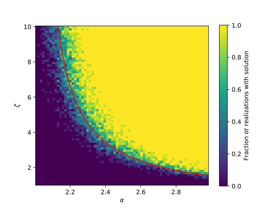 Figure 1
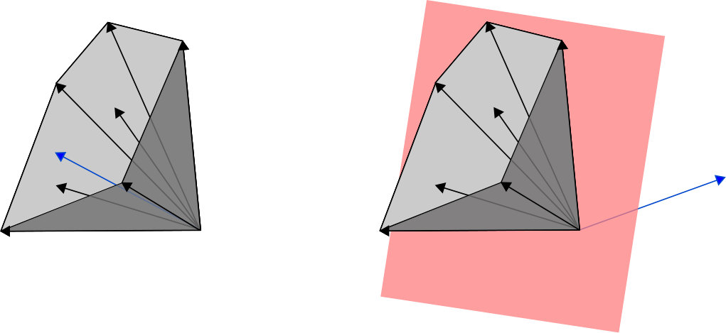 Figure 2
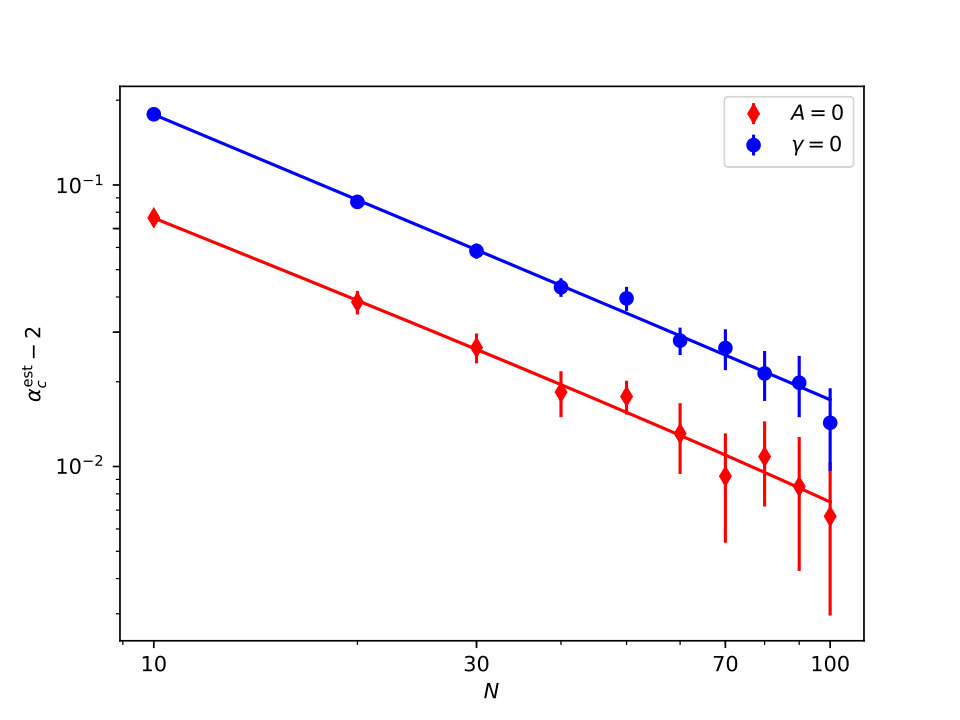 Figure 3
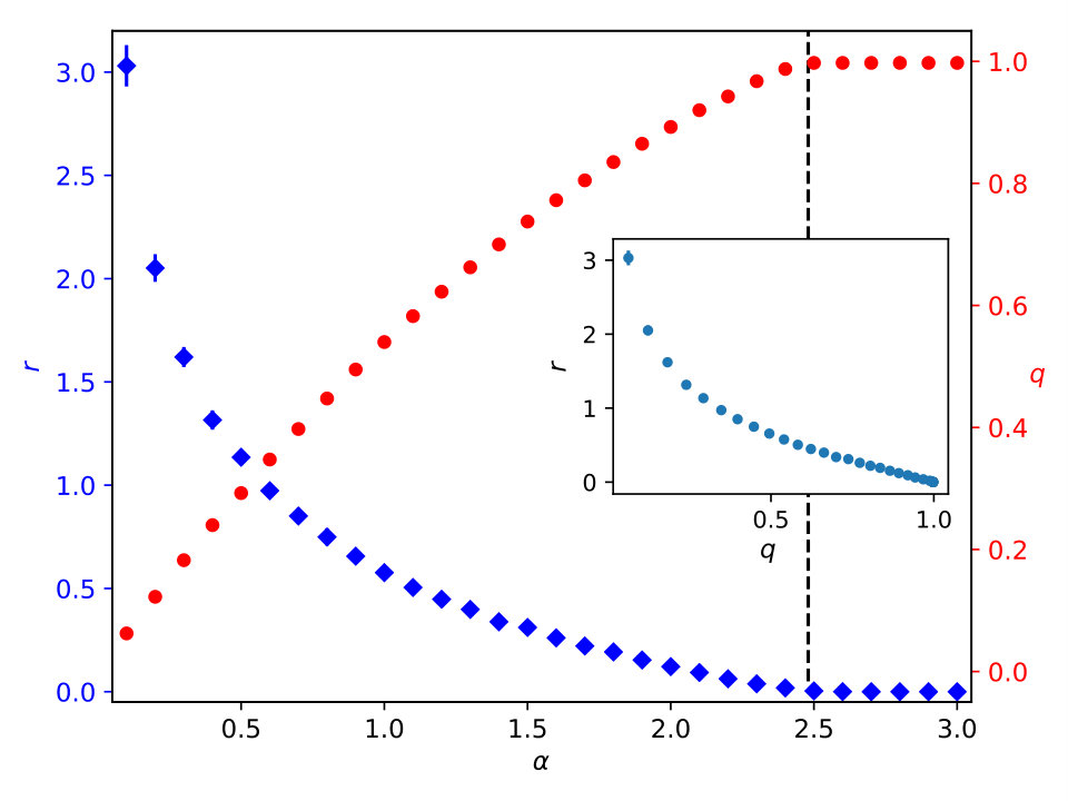 Figure 4
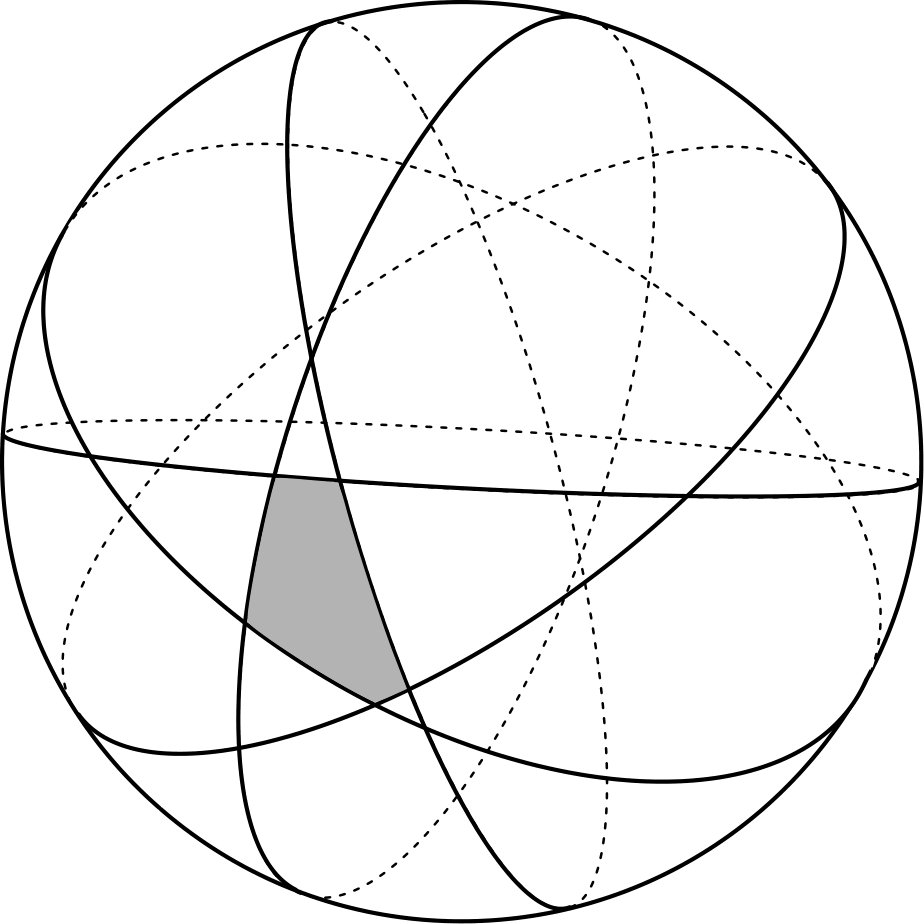 Figure 5
Peer Reviews
No public reviews on file for this paper yet. If you reviewed it on a platform where reviews are public (OpenReview, ICLR, NeurIPS, ICML), you can paste yours below so the community can read it here.
Videos
No videos yet. Explain this paper in a talk, walkthrough, or lecture? Add one.
On non-negative solutions to large systems of random linear equations
Stefan Landmann
Institute of Physics, Carl von Ossietzky University of Oldenburg, D-26111 Oldenburg, Germany
Andreas Engel
Abstract
Systems of random linear equations may or may not have solutions with all components being non-negative. The question is, e.g., of relevance when the unknowns are concentrations or population sizes. In the present paper we show that if such systems are large the transition between these two possibilities occurs at a sharp value of the ratio between the number of unknowns and the number of equations. We analytically determine this threshold as a function of the statistical properties of the random parameters and show its agreement with numerical simulations. We also make contact with two special cases that have been studied before: the storage problem of a perceptron and the resource competition model of MacArthur.
keywords:
Disordered Systems , Replica Theory , Linear Algebra
1 Introduction
Large systems of linear equations show up in many areas of physics. In particular they occur when investigating the stability of stationary states in systems with many degrees of freedom. Quite often, e.g. when considering chemical networks [1, 2] or ecological models [3, 4] only non-negative solutions are admissible since concentrations have to be positive or zero.
The interactions in such large systems are as a rule rather complex and not known in detail. On the other hand, macroscopic properties are believed not to depend on all the microscopic specifics. In situations like these models using random parameters have been extremely successful [5]. A paradigmatic case is provided by spin-glass theory [6, 7], but also problems from computational complexity [8], information theory [9] and artificial neural networks [10] have been analyzed along these lines. In these approaches emphasis is on self-averaging properties of the systems under consideration. In the thermodynamic limit their probability distributions become sharp and their averages, which are analytically accessible, characterize each typical individual realization of the randomness.
In the present paper we investigate the existence of non-negative solutions to large sets of random linear equations consisting of equations for unknowns. We are interested in the limit with staying constant. As we will show there is a sharp transition at a critical threshold from a phase in which typically no non-negative solutions exist to one where such solutions can be found. The value of is self-averaging, i.e., it depends only on the parameters characterizing the distributions of the random variables involved and not on their particular realization. Using the replica-technique we determine analytically and find very good agreement with results from numerical simulations.
The paper is organized as follows. In the next section we define the problem and map it to the determination of a random volume in -dimensional space. In section 3 we determine the typical value of this volume by a replica calculation. Section 4 discusses the transition and determines the critical line. In section 5 we consider some limiting cases and make contact with related results from the literature. In section 6 we speculate about the behavior of the system away from criticality and finally section 7 contains our conclusions.
2 Problem and notation
We consider an random matrix with entries drawn independently from a Gaussian distribution with mean and variance ,
[TABLE]
Moreover we choose a random vector composed of independent Gaussian components , with
[TABLE]
Here and in the following the brackets denote the average over the and .
We want to know whether the linear equations
[TABLE]
for the unknowns possess a solution with all components being non-negative, , which we write as .
The answer to this question clearly depends on the realization of the random numbers and . In the limit with and staying constant, however, there is a critical value of such that for there is no such solution for almost all realization of the random parameters whereas above this threshold typically one can be found. Our aim is to determine as a function of and .
It is advantageous to map the problem onto an equivalent one. Let us consider the row vectors of the matrix . All their linear combinations
[TABLE]
with non-negative coefficients form what is called the non-negative cone of the vectors . If belongs to this cone, cf. Fig. 1 left, (3) has a non-negative solution . If lies outside the cone as shown in Fig. 1 right no such solution exists. In this case there must be a hyperplane separating from the non-negative cone. Denoting the normal of this hyperplane by we therefore either have
[TABLE]
or there exists a vector with
[TABLE]
This duality is known as Farkas’ Lemma [11]. In what follows we will investigate the problem given by Eq. (6). To this end we determine the typical volume of solutions to this problem. If it is positive, (6) has solutions and consequently (5) has none. If the volume is zero no separating hyperplane exists, is part of the non-negative cone and (5) can be solved. The transition between both cases occurs when the volume shrinks to zero.
3 Typical volume of solutions to the dual problem
With each solution to (6) also with positive is a solution. In order to eliminate this trivial degeneracy it is convenient to impose the spherical constraint
[TABLE]
on the solution vectors . Our central quantity of interest is the fractional volume
[TABLE]
It comprises all normalized vectors obeying the inequalities (6), cf. Fig. 2. In (8) denotes the Heaviside function
[TABLE]
The expression for the fractional volume is rather similar to that for the version space in neural network models [12] and can be analyzed along similar lines. In particular, since involves the product of many independent random terms its logarithm is assumed to be self-averaging, i.e. in the large limit the typical value of is given by
[TABLE]
rather than by . Therefore, in order to characterize the solution space of (6) we need to determine the averaged intensive entropy
[TABLE]
This may be done using the replica trick [5] which is based on the identity
[TABLE]
is first determined for and the result needs to be continued in a meaningful way to real in order to perform the limit . For we have
[TABLE]
where the replica index runs from 1 to and the denominator accounts for the normalization (7). Using standard techniques [10] we replace the - and -functions by their integral representations:
[TABLE]
and perform the averages over and
[TABLE]
The integrals over the , the auxiliary variables and their conjugates can be decoupled by introducing the order parameters
[TABLE]
The expression for the -th power of the fractional volume then acquires the form
[TABLE]
with the auxiliary functions
[TABLE]
and
[TABLE]
To determine the entropy (11) we only need the asymptotics of this expression for so that the integrals in (17) may be calculated by the saddle-point method. The term can be neglected in this limit and will be dropped.
The solution space of Eq. (6) is connected, we therefore assume a replica-symmetric saddle-point and use the ansätze
[TABLE]
Keeping in mind that for the final limit only terms up to order are needed the expressions for and simplify considerably. We find
[TABLE]
Here the Gaussian measure was introduced and the abbreviations
[TABLE]
were used. Similar manipulations yield for
[TABLE]
Also the other terms in (17) can be simplified using (20) and (21). As a consequence the saddle-point equations for the order parameters become algebraic and these parameters can be eliminated. Introducing
[TABLE]
we finally get
[TABLE]
The saddle-point values of and have to be determined numerically. Note that the final expression (26) for the averaged entropy depends on the parameters and characterizing the distributions of and only through the combination that gives the ratio between the relative variances of and .
4 The transition point
At the transition point the typical volume becomes zero, i.e. the average entropy tends to minus infinity. It is possible to extract this point from the numerical extremalization in (26). However, the analysis can be simplified by observing that with shrinking to zero the typical overlap between two different solutions as defined in (16) tends to one. To leading order in we get
[TABLE]
implying
[TABLE]
Keeping only the most divergent terms near the transition we thus find
[TABLE]
The saddle-point equation with respect to gives
[TABLE]
whereas the one with respect to results in
[TABLE]
Together with (30) this yields
[TABLE]
Eqs. (30) and (32) give a parametric description of the transition line . It is shown in Fig. 3 together with results from numerical solutions of Eq. (3). There is good agreement between the analytical prediction and simulation results.
5 Special cases
The basic problems (5) and (6) respectively are rather general. Some special cases have been studied previously in different settings.
5.1 Relation to the storage problem of a perceptron
From the numerical analysis of (26) one finds that for large the saddle-point value of tends to zero such that also . In this limit we hence find
[TABLE]
which coincides with Gardner’s famous expression describing the storage problem of a perceptron [12]. In this problem one is given random input patterns and corresponding outputs and has to find a synaptic vector such that
[TABLE]
for all . For more details see [10].
There are two situations that make the equivalence between this storage problem for the perceptron and our dual problem (6) for particularly clear. Firstly, let us consider the case such that for all . We then decompose where the entries of are constant while the entries of are i.i.d. random gaussian variables with zero mean and variance . Then, (6) requires
[TABLE]
The condition restricts all to lie on the ’negative’ half of the -sphere. From high-dimensional geometry it is known that for the volume spanned by the vectors on the -sphere is tightly concentrated around the equator. Therefore, it may be assumed that without reducing the fractional volume 111This is substantiated by the fact that the saddle-point value of as defined in (16) is zero in this case.. Effectively the conditions therefore become
[TABLE]
In this form they are equivalent to the storage problem for patterns. For the influence of the additional pattern can be neglected. The critical value of in the storage problem is known to be [12]. Figure 4 shows results from a finite size analysis of for the system (3) with . For we obtain corroborating the equivalence between the two problems in the large limit.
Secondly, our analysis reduces to the storage problem of the perceptron if . In this case Eq.(6) acquires the form
[TABLE]
Clearly, the first condition is equivalent to the storage problem for patterns. To show that the second one does not reduce the fractional volume for large we split it into and and require these two constraints separately. Even this more severe restriction is only equivalent to two additional patterns, , which in the limit is again irrelevant. Figure 4 shows that also in this case the finite size analysis of is in perfect agreement with the result from the storage problem of the perceptron.
5.2 MacArthur model of resource competition
A classical model to describe biodiversity in ecological systems considers a number of species that compete for a number of different resources [13]. The species differ in their ability to live on the various resources which is described by a matrix of metabolic strategies . The elements of characterize the ease with which species may consume resource . Resources are provided by certain fixed influxes from the environment. For sufficiently large there is a stationary state of the system with species concentrations in which the overall consumption of each resource is exactly balanced by its influx:
[TABLE]
Since moreover all must be either positive (if the species survives) or zero (if the species got extinct) the vector has to fulfill Eq. (5).
The MacArthur model has been studied extensively for systems with only a few species and correspondingly few resources. On the other hand, realistic biological systems may involve hundreds of species and resources. In a very interesting recent paper [14] a random version of MacArthur’s model was analyzed in the limit . To this end the elements of the matrix of metabolic strategies were chosen independently of each other as either one with probability or zero with probability . Large values of hence describe communities of universalists that can live from many different resources, small values of stand for systems consisting mostly of specialists. The resource influx was modelled as a Gaussian random vector with elements of average one and variance . Interestingly, in this variant of the MacArthur model a transition was found from a so-called vulnerable phase at low potential biodiversity (small ) to a so-called shielded phase at large . In the vulnerable phase the species are unable to use all available resources properly, Eq. (38) cannot be fulfilled, less than species survive, and variations in the resource influxes have a direct impact on each species. Contrarily, in the shielded phase the species form a collective field that guards them from changes in the external conditions, the maximal possible number of species survives [15], and Eq. (38) is satisfied. This phase is a striking example for the emergence of cooperation in a purely competitive system [16]. The transition found in [14] is equivalent to the one discussed in the present paper for , , and . For more details see [17].
6 Making contact away from criticality
The Farkas Lemma connects the two dual problems (5) and (6): whenever there is a solution to one there is none to the other. Therefore the threshold values for both problems coincide. However, from the solution space analysis described in section 3 more details may be extracted. For , e.g., there are many different solutions to problem (6). The order parameter which can be determined from the numerical extremalization in (26) is then strictly smaller than one and provides a measure of the variability between different solutions to (6). At the same time the dual problem (5) is unsolvable as demonstrated by a non-zero residual norm
[TABLE]
This residual norm in some sense quantifies how far away problem (5) is from its threshold of solvability. It is tempting to speculate about a connection between and . If is rather small there are many different solutions to (6). Accordingly, problem (5) should be ’far from being solvable’ corresponding to a large value of . For near to one, on the other hand, there is not much freedom left for different solutions of (5) and small values of are likely. We have tested this conjecture with the help of numerical simulations. The results shown in Fig. 5 indeed suggest a monotonous relation between and .
Equivalent considerations apply to the region . Here (6) is unsolvable and its solution space is empty. By a slight generalization of the techniques used in section 3 it is possible to determine the minimal number of violated inequalities in (6) [18]. It is an open question whether this number may be related to the variability between different solutions of (5) for .
7 Conclusion
In the present paper we investigated under which conditions a large set of random linear equations for unknowns typically possesses a non-negative solution. This is a rather general question with relevance for a number of different problems in statistical mechanics. It is also an active area of research in mathematics on its own [19, 20].
With the help of Farkas’ lemma we mapped the problem onto the determination of the typical size of a random volume in high-dimensional space which could be characterized analytically using methods from the statistical physics of disordered systems. Our main result is a sharp transition in the limit that separates a phase where the linear system typically has no non-negative solution to one in which such a solution can be found with probability one. The analytical result for the transition line agrees very well with the outcome of numerical simulations. Special cases of the transition have been discussed previously in the literature in connection with the storage capacity of a large perceptron and with a random variant of MacArthurs resource competition model.
In order to keep the calculations simple we assumed Gaussian distributions for the random parameters. For the elements of the coefficient matrix this assumption is not crucial. As in related mean-field models any distribution of these elements with finite moments would give similar results depending only on their first two cumulants. This is, e.g., exemplified by the application to MacArthurs model. The statistical properties of the inhomogeneity vector are more subtle and similar generalizations to different distributions deserve further investigation.
The dual problem related to the typical size of a random volume in -space can also be studied for values of different from the threshold . It were rather interesting if this knowledge could be used to quantitatively characterize the original problem away from criticality, i.e. deeply in the solvable or unsolvable phase. We presented preliminary numerical evidence that this may be possible but more work is needed to substantiate this connection.
Acknowledgement: Financial support from the German Science Foundation under project EN 278/10-1 is gratefully acknowledged. A.E. is deeply grateful for numerous inspiring discussions and genial conversations with Chris van den Broeck he enjoyed over many years.
The reference list from the paper itself. Each links out to its DOI / PubMed record.
- 1[1] M. Polettini, M. Esposito, Irreversible thermodynamics of open chemical networks. I. Emergent cycles and broken conservation laws, The Journal of chemical physics 141 (2014) 024117.
- 2[2] J. Schnakenberg, Simple chemical reaction systems with limit cycle behaviour, Journal of Theoretical Biology 81 (3) (1979) 389–400.
- 3[3] R. M. May, Will a large complex system be stable?, Nature 238 (1972) 413.
- 4[4] M. Eigen, P. Schuster, The hypercycle, Naturwissenschaften 65 (1) (1978) 7–41.
- 5[5] M. Mézard, G. Parisi, M. Virasoro, Spin glass theory and beyond, World Scientific Publishing Company, 1987.
- 6[6] S. F. Edwards, P. W. Anderson, Theory of spin glasses, Journal of Physics F: Metal Physics 5 (5) (1975) 965.
- 7[7] D. Sherrington, S. Kirkpatrick, Solvable model of a spin-glass, Physical Review Letters 35 (26) (1975) 1792.
- 8[8] R. Monasson, R. Zecchina, S. Kirkpatrick, B. Selman, L. Troyansky, Determining computational complexity from characteristic ‘phase transitions’, Nature 400 (1999) 133–137.