The surrogate matrix methodology: Low-cost assembly for isogeometric analysis
Daniel Drzisga, Brendan Keith, Barbara Wohlmuth

TL;DR
This paper introduces a low-cost surrogate matrix methodology for isogeometric analysis that significantly reduces assembly time by performing limited quadrature and interpolating remaining matrix entries, with negligible impact on accuracy.
Contribution
The paper presents a novel surrogate matrix approach that reduces computational cost in IGA by combining selective quadrature with B-spline interpolation, easily integrable into existing software.
Findings
Over fifty-fold reduction in assembly time.
Negligible impact on solution accuracy.
Applicable to various PDE problems.
Abstract
A new methodology in isogeometric analysis (IGA) is presented. This methodology delivers low-cost variable-scale approximations (surrogates) of the matrices which IGA conventionally requires to be computed from element-scale quadrature formulas. To generate surrogate matrices, quadrature must only be performed on certain elements in the computational domain. This, in turn, determines only a subset of the entries in the final matrix. The remaining matrix entries are computed by a simple B-spline interpolation procedure. Poisson's equation, membrane vibration, plate bending, and Stokes' flow problems are studied. In these problems, the use of surrogate matrices has a negligible impact on solution accuracy. Because only a small fraction of the original quadrature must be performed, we are able to report beyond a fifty-fold reduction in overall assembly time in the same software. The…
Click any figure to enlarge with its caption.
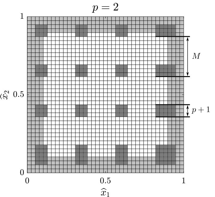 Figure 1
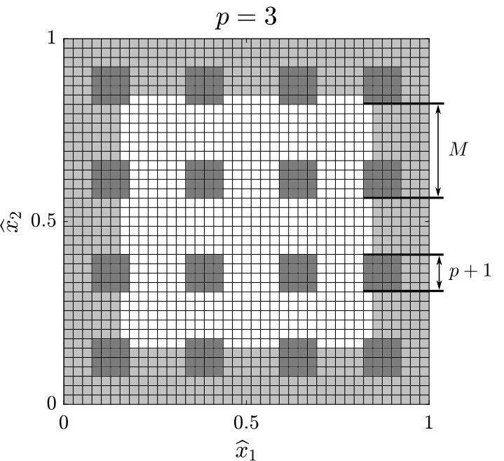 Figure 2
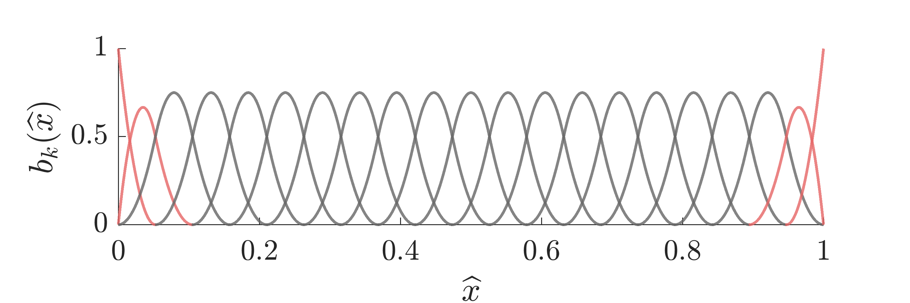 Figure 3
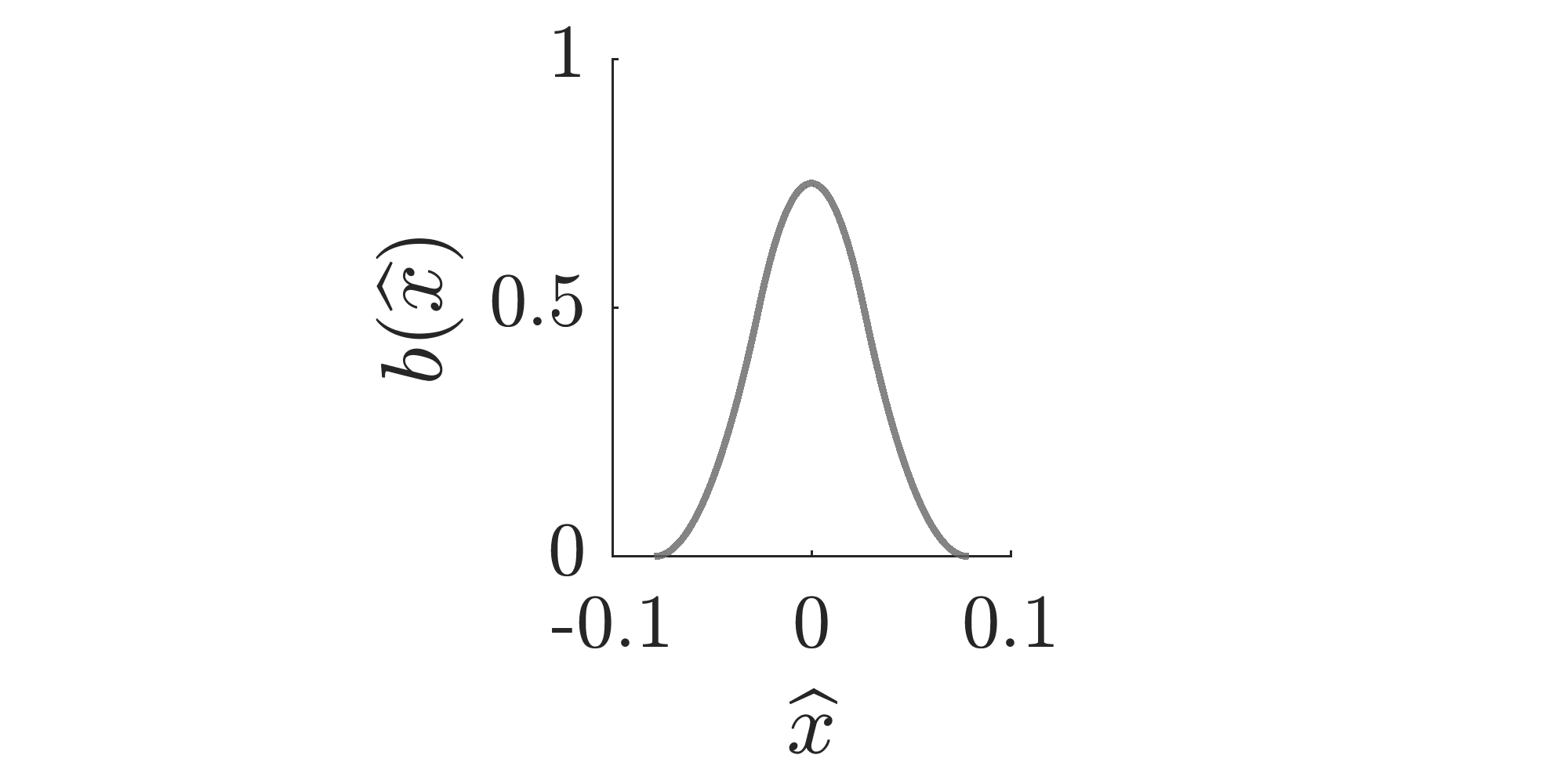 Figure 4
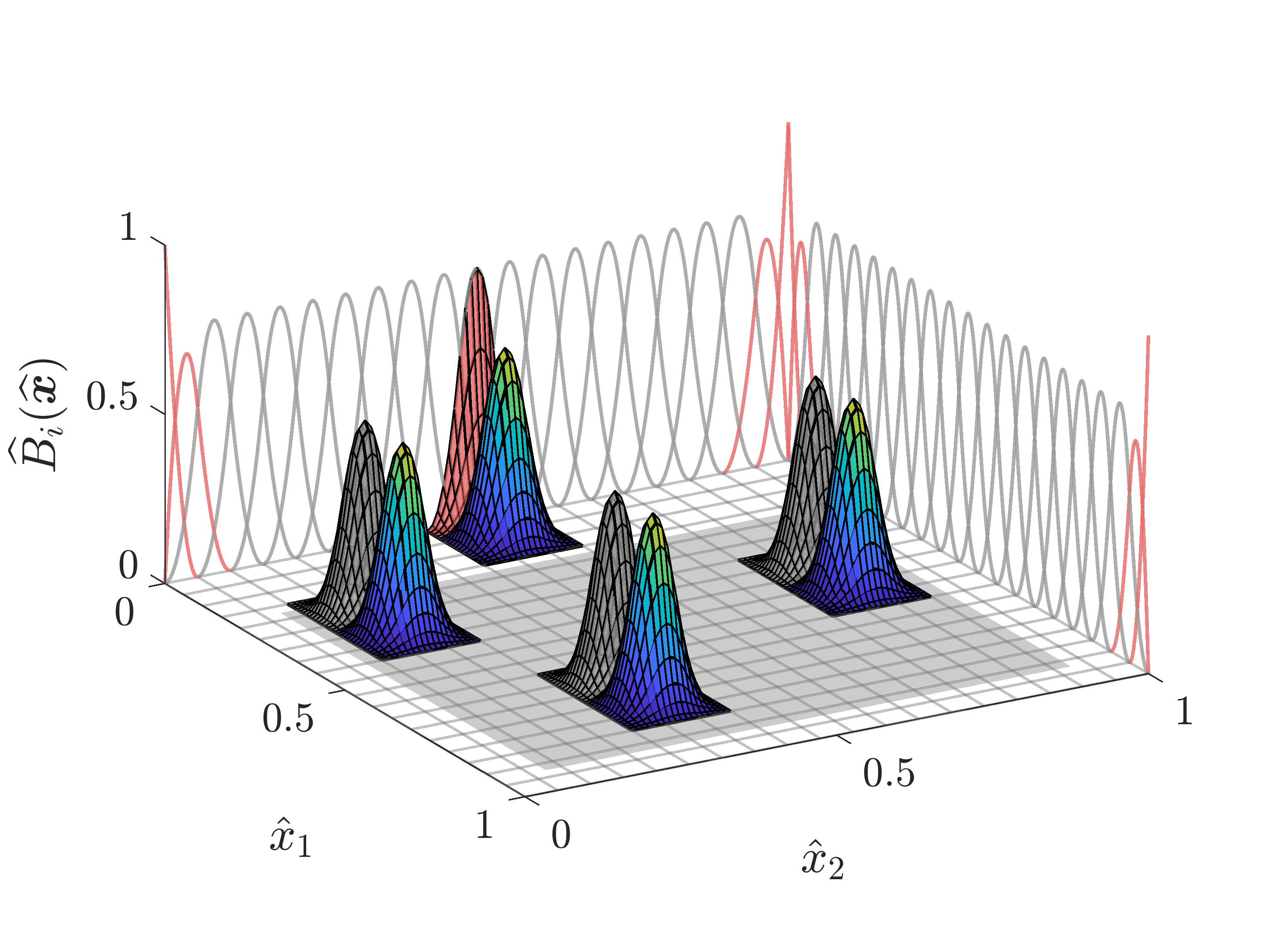 Figure 5
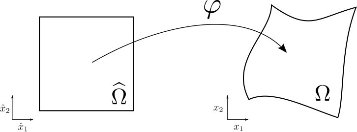 Figure 6
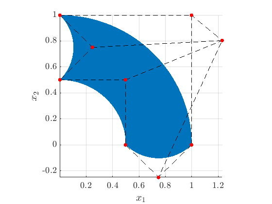 Figure 7
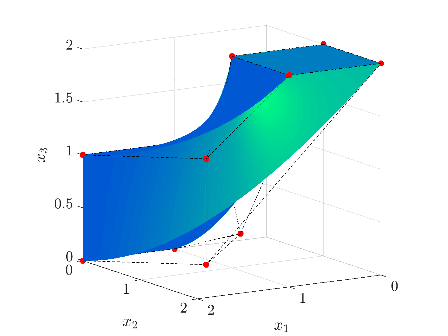 Figure 8
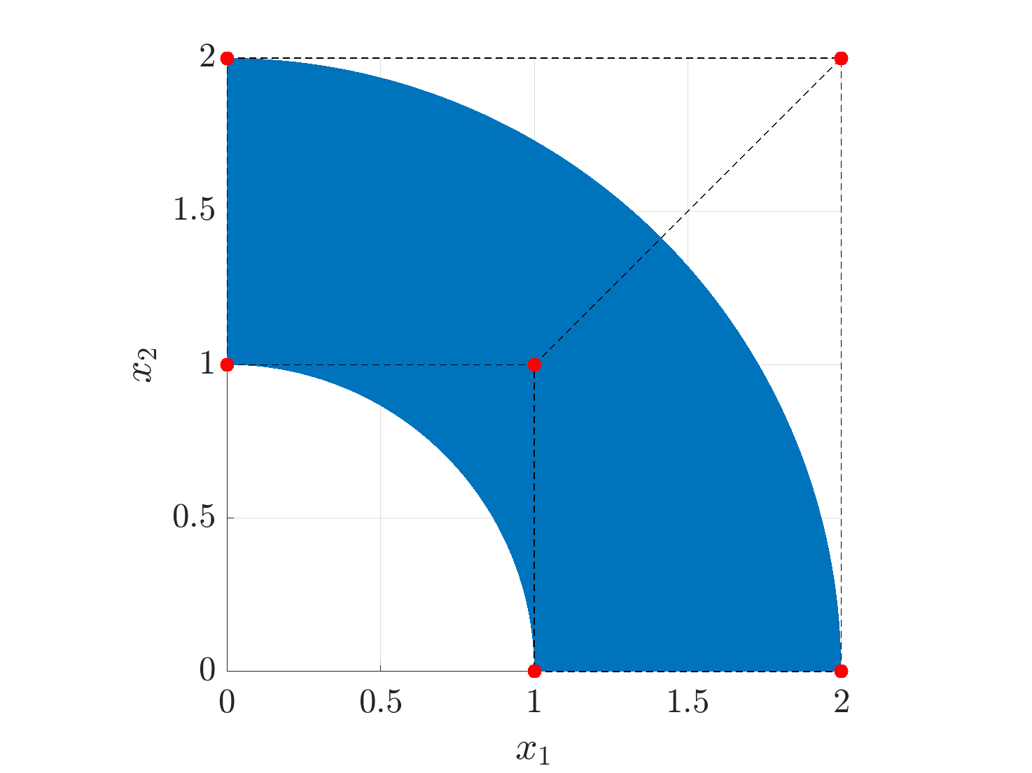 Figure 9
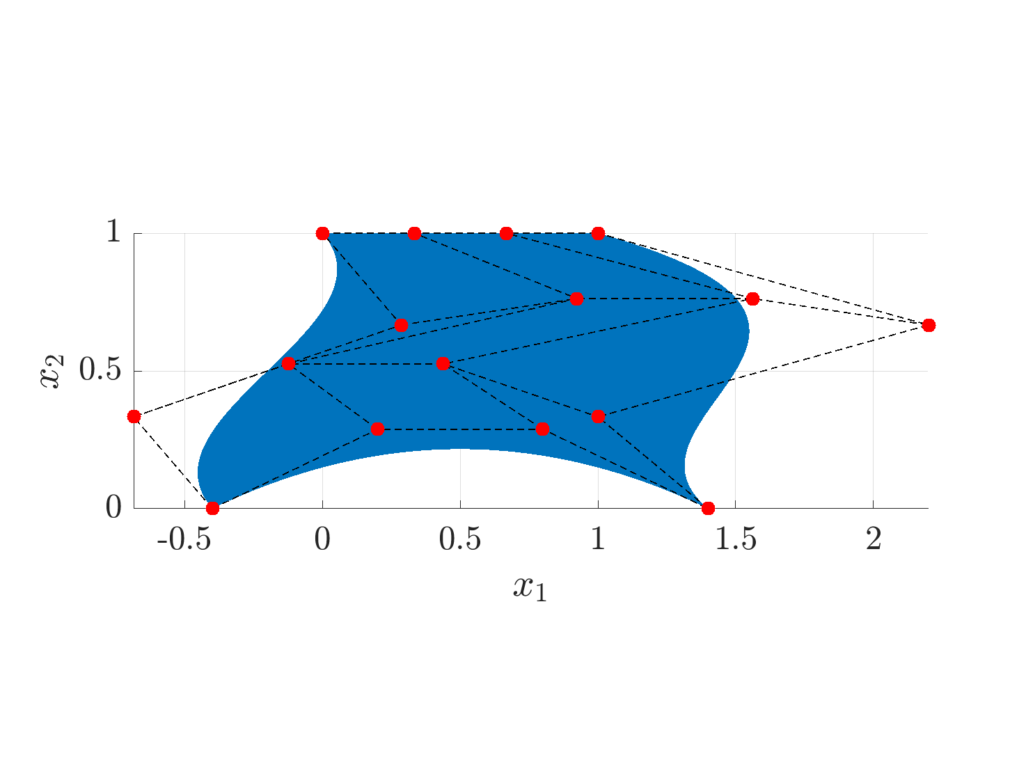 Figure 10
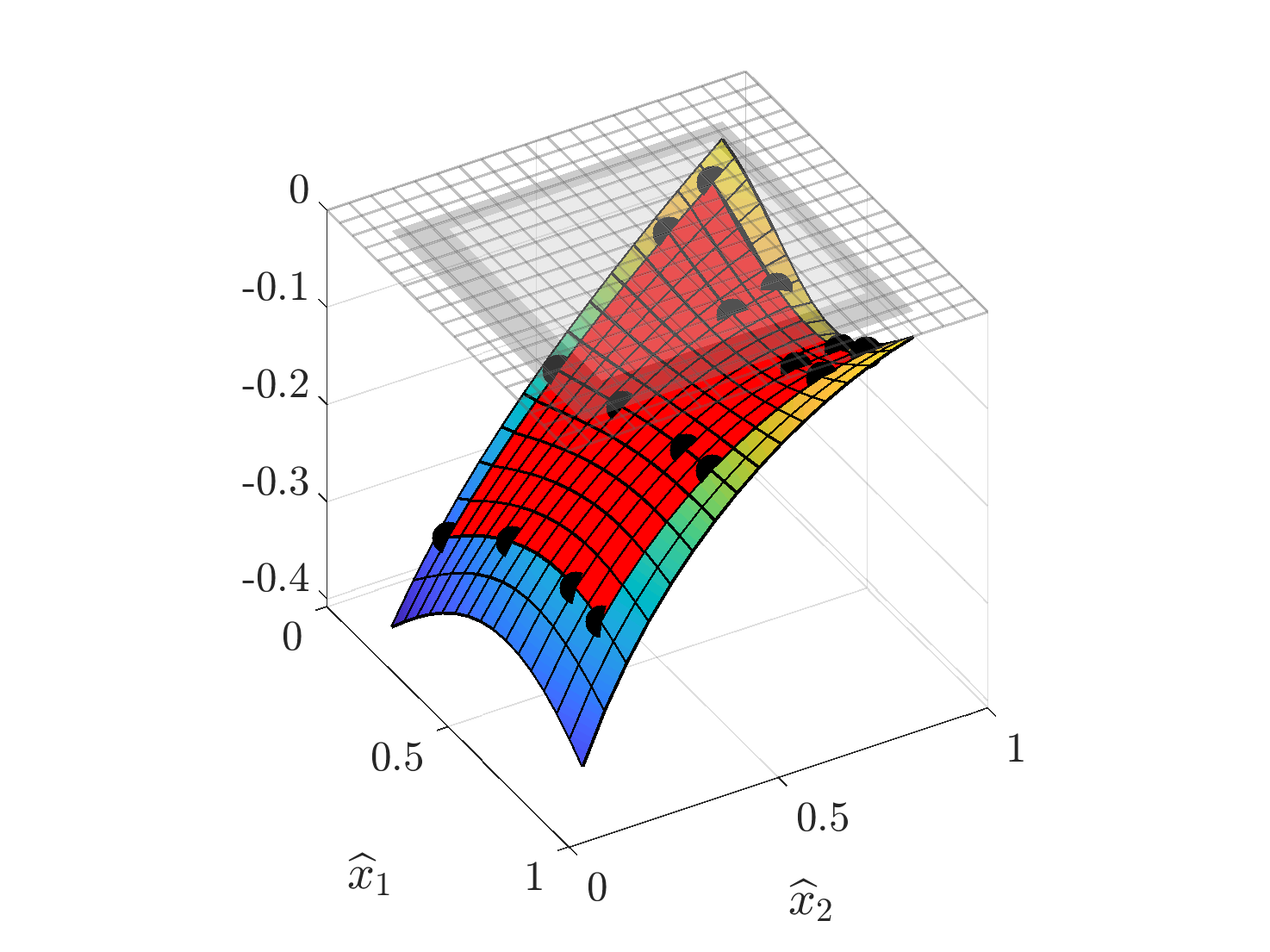 Figure 11
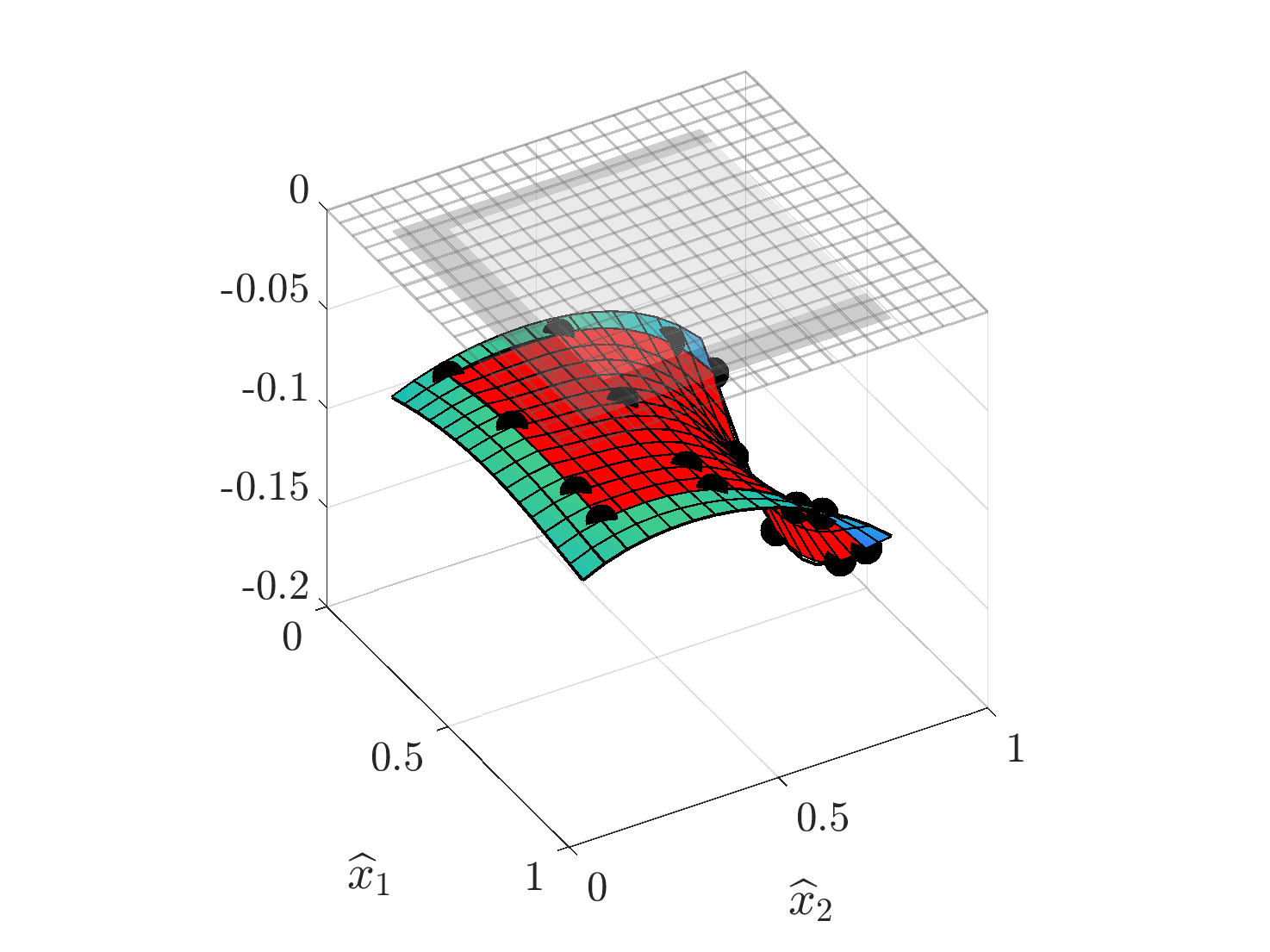 Figure 12
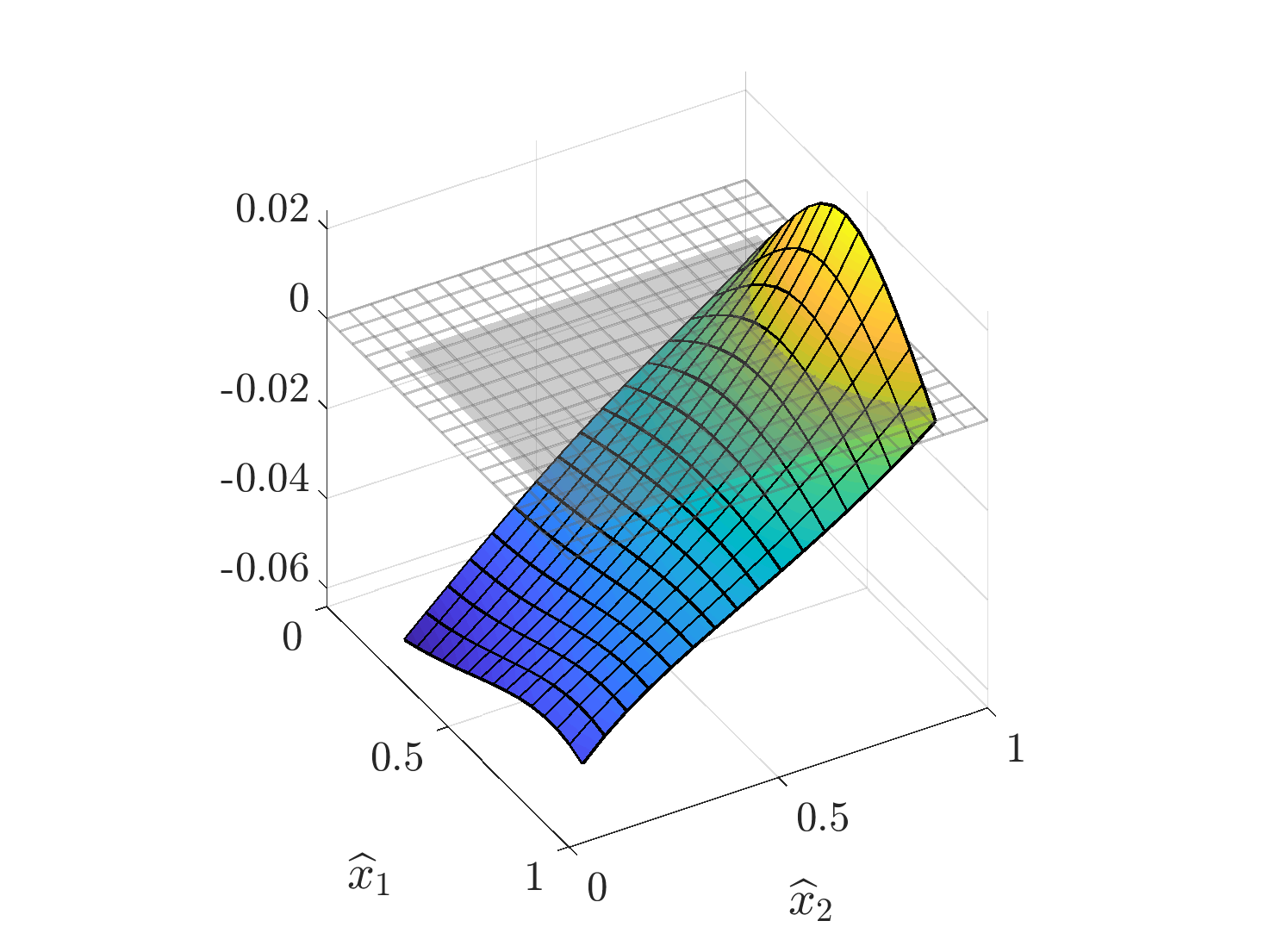 Figure 13
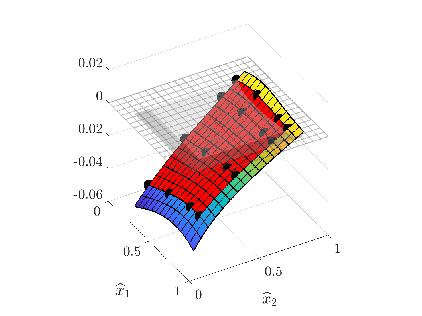 Figure 14
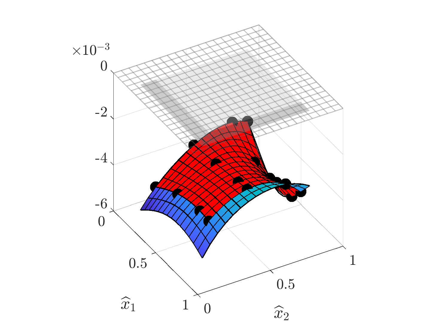 Figure 15
 Figure 16
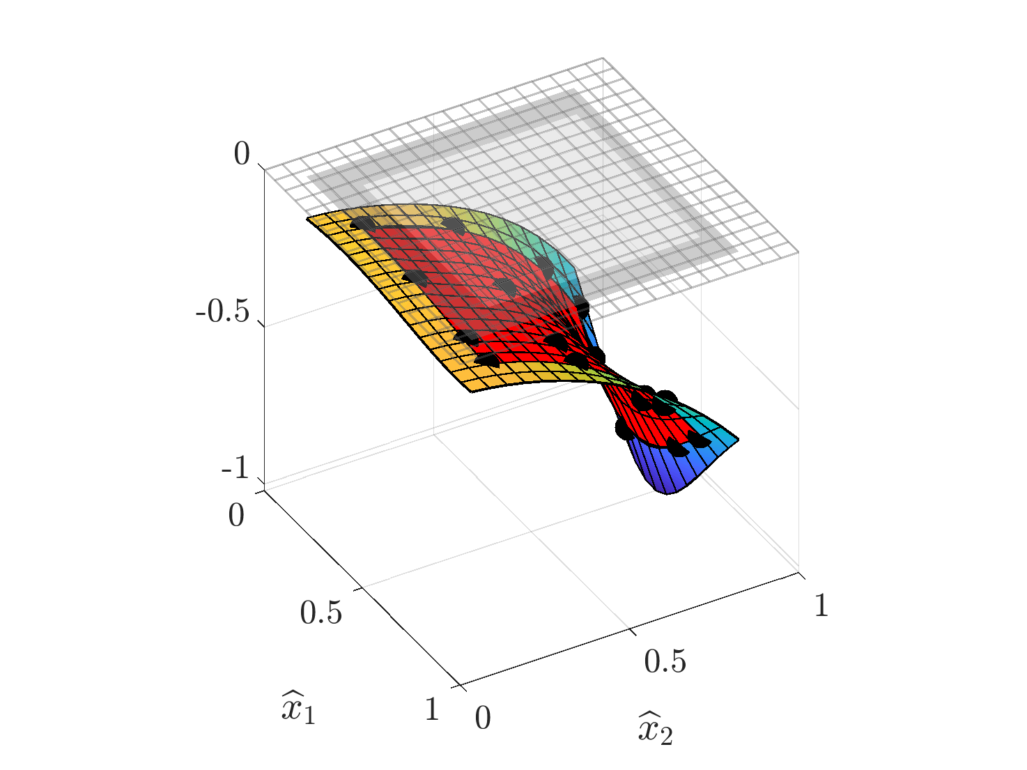 Figure 17
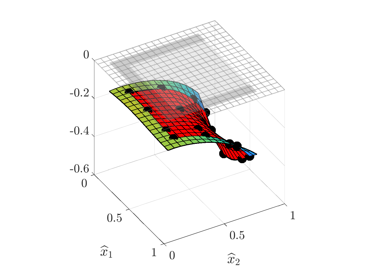 Figure 18
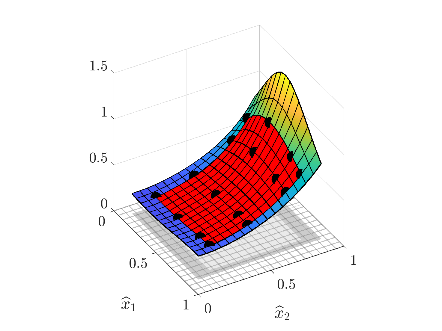 Figure 19
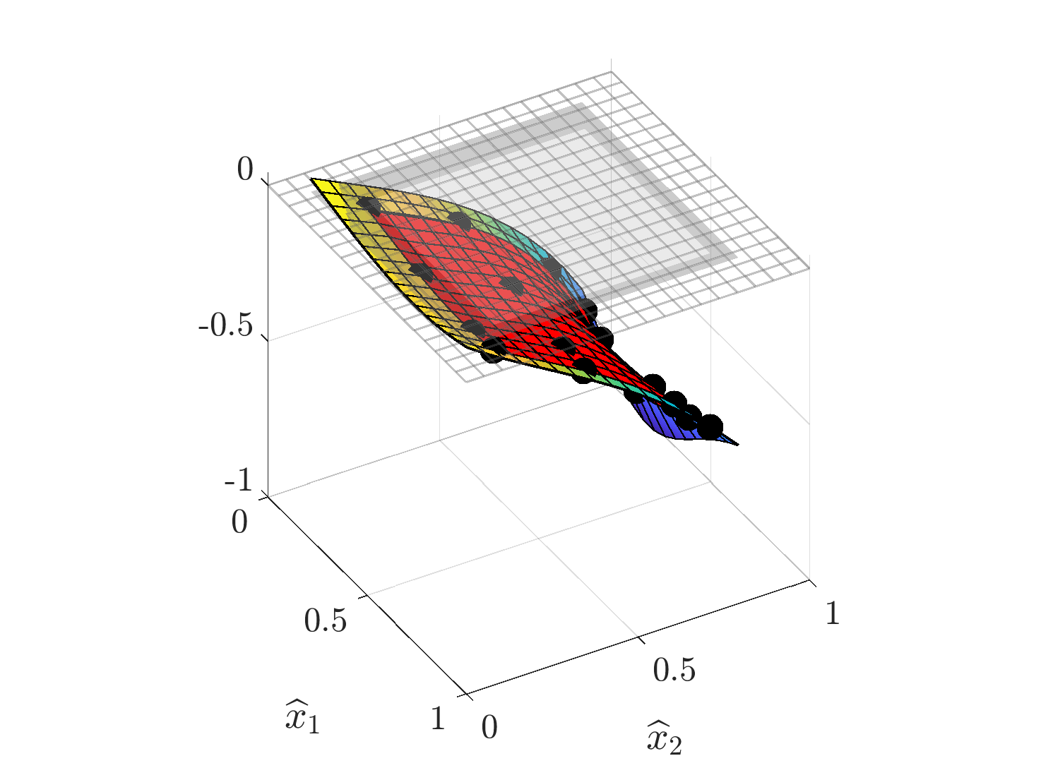 Figure 20
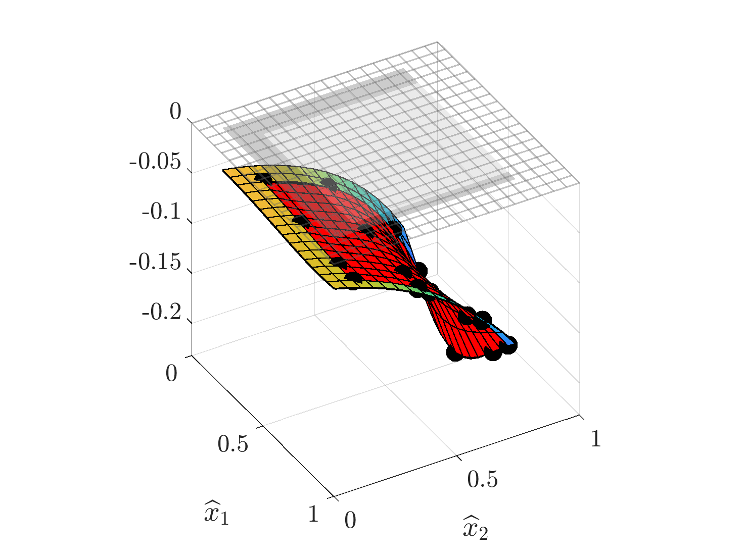 Figure 21
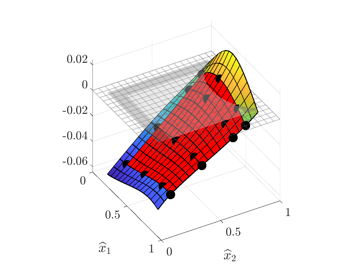 Figure 22
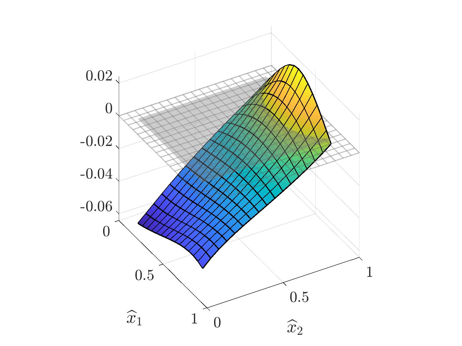 Figure 23
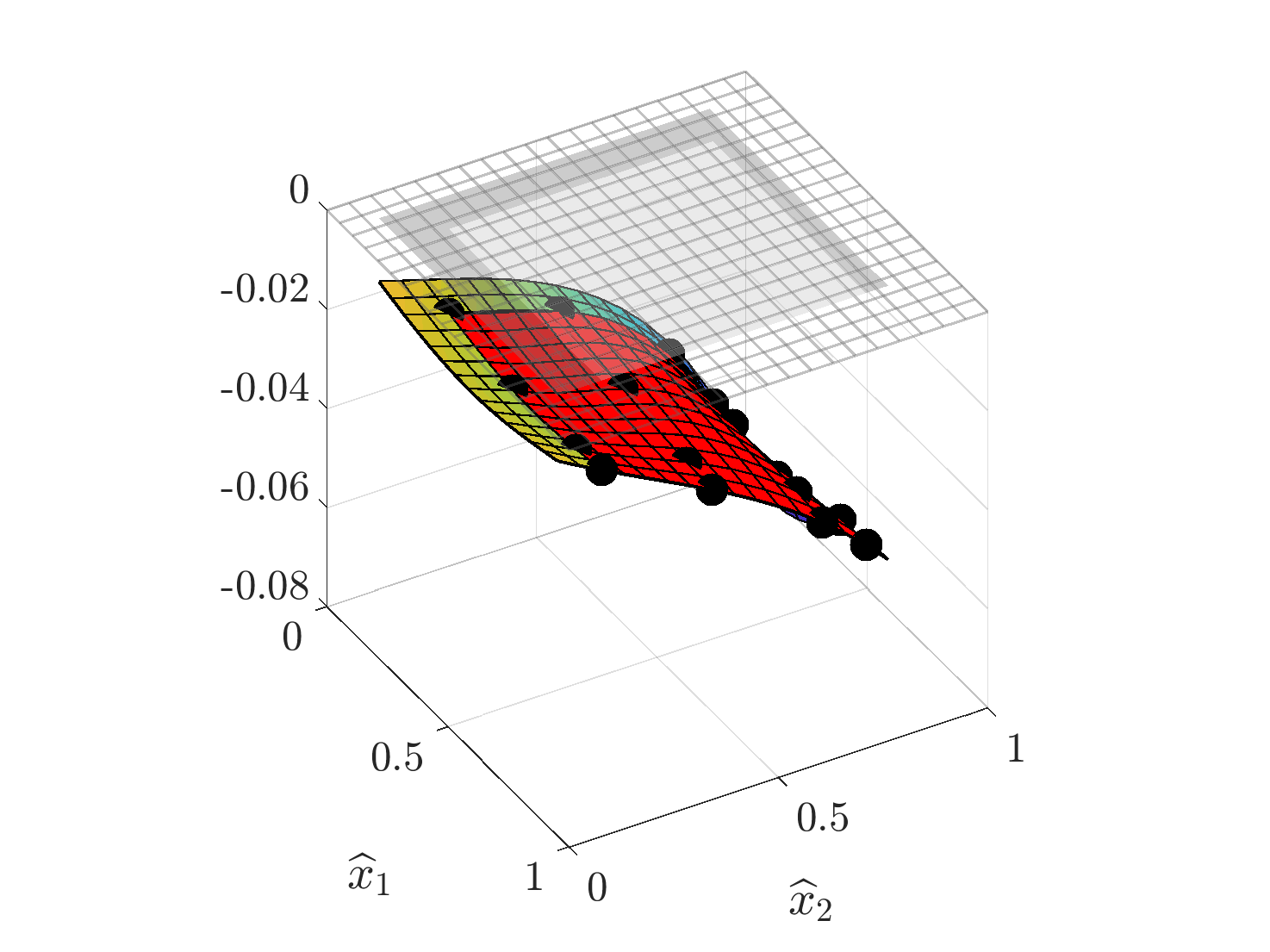 Figure 24
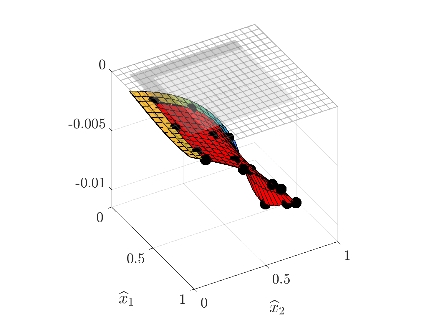 Figure 25
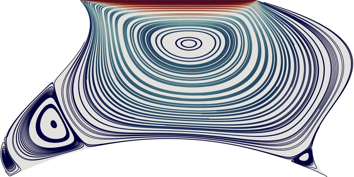 Figure 26
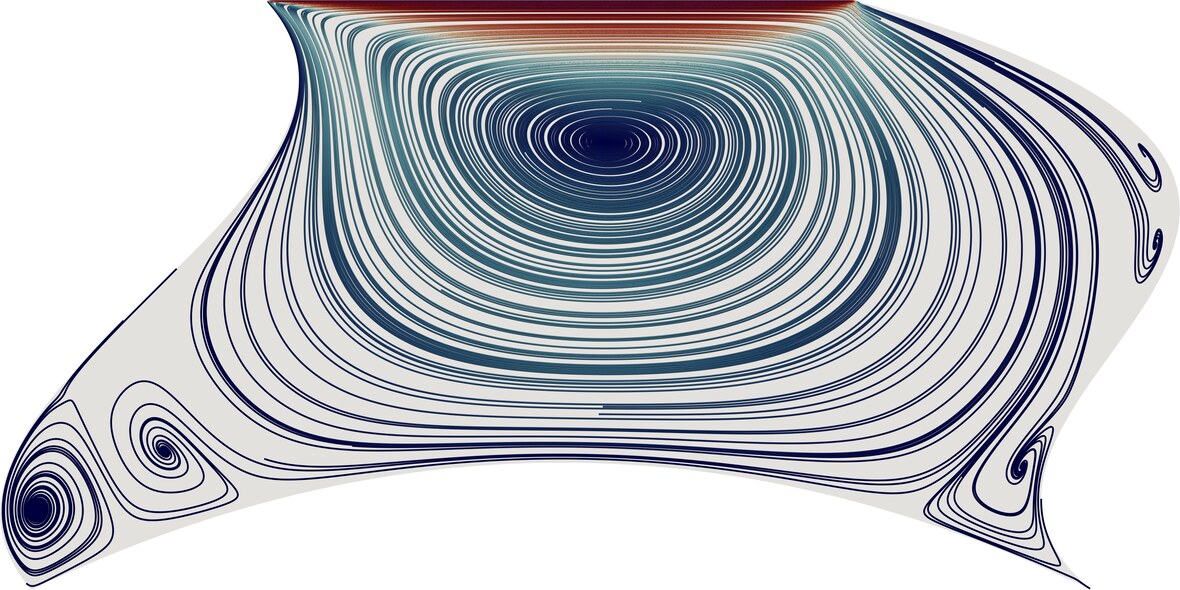 Figure 27
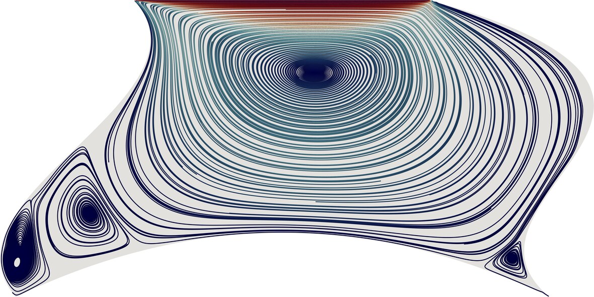 Figure 28
 Figure 29
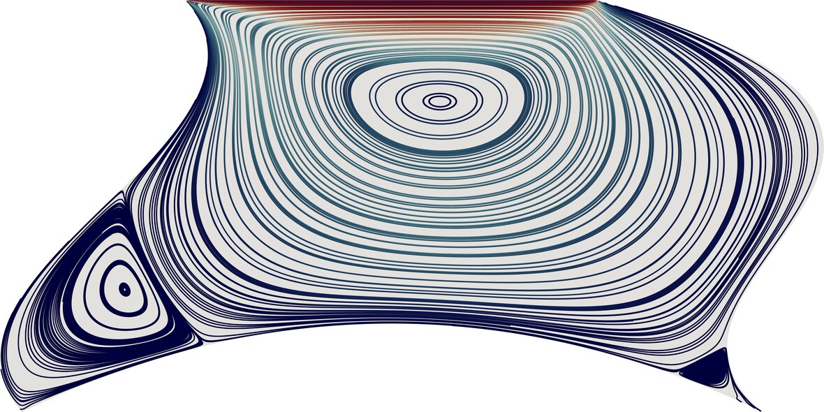 Figure 30
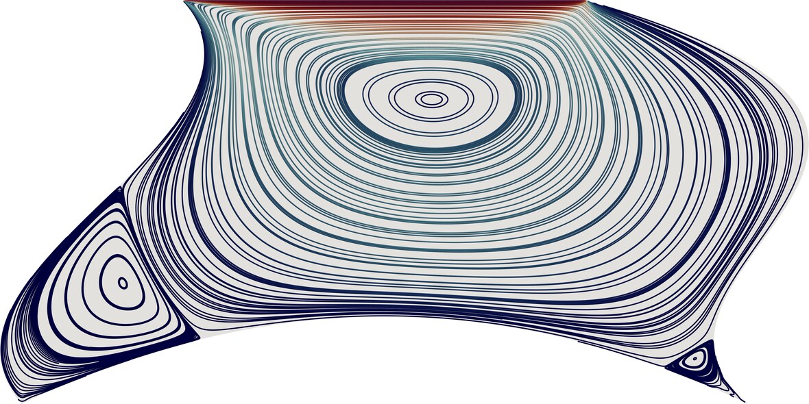 Figure 31
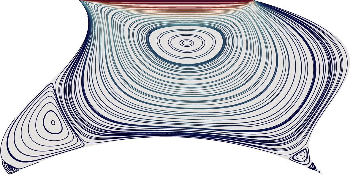 Figure 32
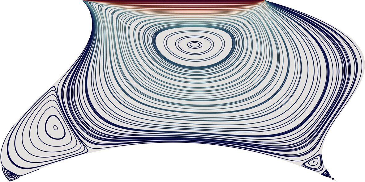 Figure 33
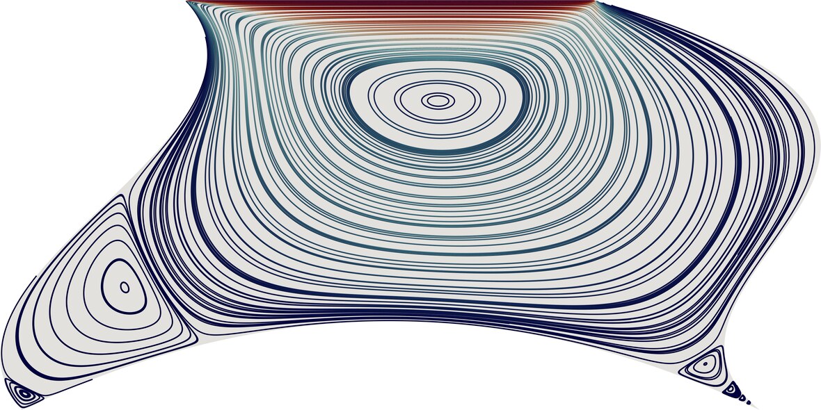 Figure 34
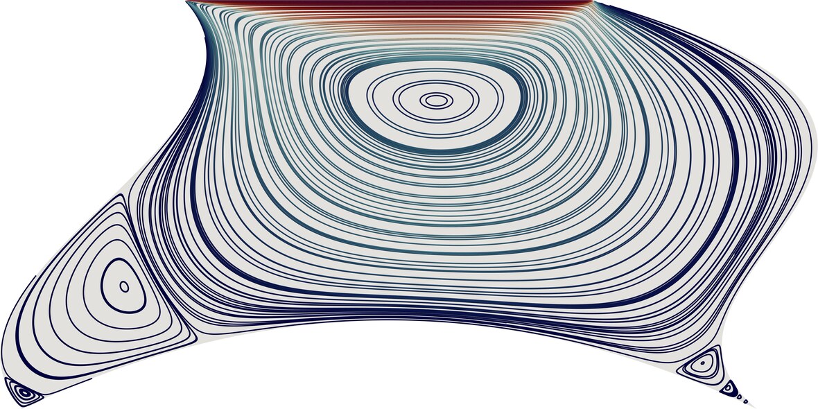 Figure 35
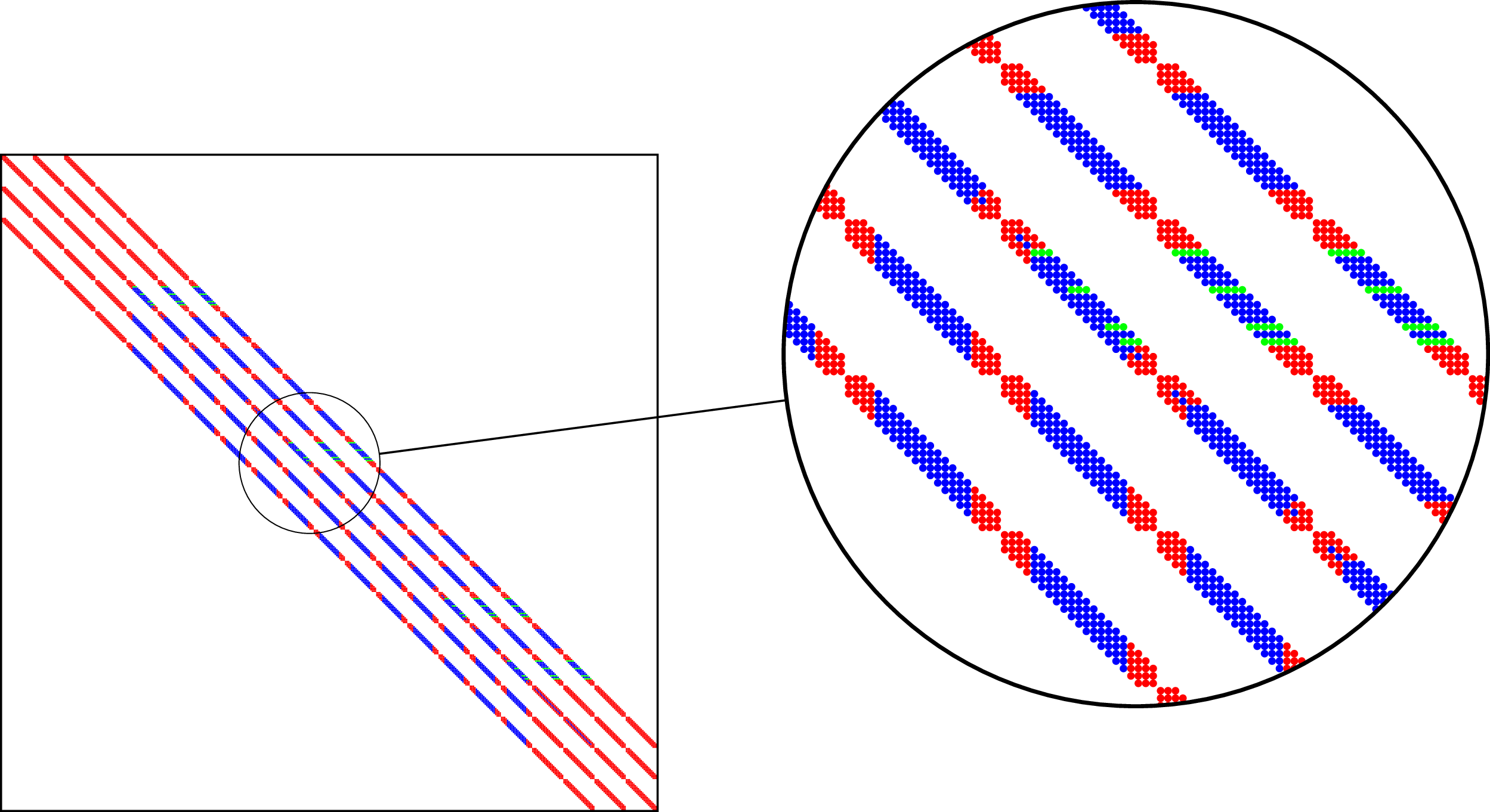 Figure 36
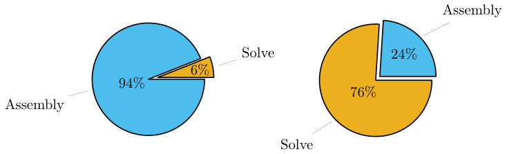 Figure 0
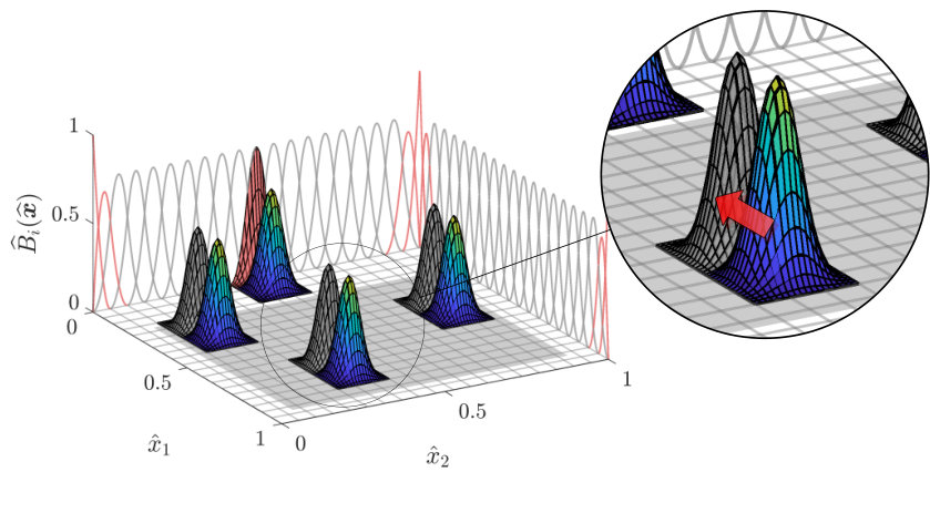 Figure 1
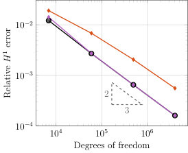 Figure 10
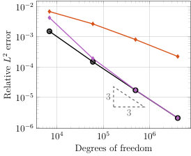 Figure 11
Peer Reviews
No public reviews on file for this paper yet. If you reviewed it on a platform where reviews are public (OpenReview, ICLR, NeurIPS, ICML), you can paste yours below so the community can read it here.
Videos
No videos yet. Explain this paper in a talk, walkthrough, or lecture? Add one.
\NewEnviron
scaletikzpicturetowidth[1]\BODY
The surrogate matrix methodology: Low-cost assembly for isogeometric analysis
Daniel Drzisga Lehrstuhl für Numerische Mathematik, Fakultät für Mathematik (M2), Technische Universität München, Garching bei München (, , ) [email protected]
Brendan Keith11footnotemark: 1
Barbara Wohlmuth11footnotemark: 1
(with support in ; The correspond to the midpoints of each function .; We define; by; ^a; as; Figure 7 presents graphs of stencil functions, and their surrogates obtained by B-spline interpolation for various . The stencil functions are generated by an isogeometric NURBS basis and the symmetric bilinear form 8.; , with each ; and, moreover, . The result follows from Lemma 4.1 using .; will; ^w; ^v; ^a; ^ωδ; First, the sampling length and the sampling points need to be specified. For this purpose, we introduce the sampling parameter M ̄\in\mathbb{N} which relates the small scale to the coarse scale via .; out; needs; Some of the diagonal entries are drawn in blue due to the modification of preserving the kernel.; Some of the diagonal entries are drawn in blue due to the modification of preserving the kernel.; *Dirichlet boundary conditions are enforced for surrogate methods in the standard way; that is, by eliminating dofs from the original linear system. As usual, let be the full matrix without any consideration for boundary conditions. Without loss of generality, we may assume that all the smallest global indices correspond to the set of interior dofs, denoted by , and all of the largest correspond to the set of Dirichlet dofs, denoted by . The unconstrained linear system, , may then be written in block form as follows:
(23)
Recall that all cardinal basis functions vanish at domain boundary . Therefore, following definition 18c, and , where and are the corresponding submatrices of the standard stiffness matrix . Furthermore, because the values of are prescribed, 23 may be reduced to the linear system . This reduced system may be solved to determine all the unprescribed solution coefficients, . *; * In this proof, we will use the symbols “” and “” to denote upper bounds and equivalence, respectively, up to constants depending at most on and . For each , let be the set of indices such that and notice that . We begin with the observation that \sum_{i}\big{(}\mathsf{A}_{ij}-\widetilde{\mathsf{A}}_{ij}\big{)}=\sum_{j}\big{(}\mathsf{A}_{ij}-\widetilde{\mathsf{A}}_{ij}\big{)}=0. With these two identities in hand, we find that
(27)
\displaystyle=-\frac{1}{2}\,{\sum_{i,j}}\big{(}\mathsf{A}_{ij}-\widetilde{\mathsf{A}}_{ij}\big{)}(\mathsf{v}_{i}-\mathsf{v}_{j})\hskip 0.25pt({\mathsf{w}_{i}}-\mathsf{w}_{j})
\displaystyle\leq|\mathsf{A}-\widetilde{\mathsf{A}}|_{\operatorname*{\vphantom{p}max}}\sum_{i}\Bigg{(}\sum_{j\in\mathcal{I}(i)}|\mathsf{v}_{i}-\mathsf{v}_{j}|^{2}\Bigg{)}^{\mathchoice{\raisebox{0.0pt}{\displaystyle{}\mathchoice{\raisebox{-0.2pt}{}}{\raisebox{-0.2pt}{}}{\raisebox{-0.2pt}{}}{\raisebox{-0.2pt}{}}/\mathchoice{\raisebox{-0.1pt}{}}{\raisebox{-0.1pt}{}}{\raisebox{-0.1pt}{}}{\raisebox{-0.1pt}{}}}}{\raisebox{0.0pt}{\textstyle{}\mathchoice{\raisebox{-0.2pt}{}}{\raisebox{-0.2pt}{}}{\raisebox{-0.2pt}{}}{\raisebox{-0.2pt}{}}/\mathchoice{\raisebox{-0.1pt}{}}{\raisebox{-0.1pt}{}}{\raisebox{-0.1pt}{}}{\raisebox{-0.1pt}{}}}}{\raisebox{0.0pt}{\scriptstyle{}\mathchoice{\raisebox{-0.2pt}{}}{\raisebox{-0.2pt}{}}{\raisebox{-0.2pt}{}}{\raisebox{-0.2pt}{}}/\mathchoice{\raisebox{-0.1pt}{}}{\raisebox{-0.1pt}{}}{\raisebox{-0.1pt}{}}{\raisebox{-0.1pt}{}}}}{\raisebox{0.0pt}{\scriptscriptstyle{}\mathchoice{\raisebox{-0.2pt}{}}{\raisebox{-0.2pt}{}}{\raisebox{-0.2pt}{}}{\raisebox{-0.2pt}{}}/\mathchoice{\raisebox{-0.1pt}{}}{\raisebox{-0.1pt}{}}{\raisebox{-0.1pt}{}}{\raisebox{-0.1pt}{}}}}}\Bigg{(}\sum_{j\in\mathcal{I}(i)}|\mathsf{w}_{i}-\mathsf{w}_{j}|^{2}\Bigg{)}^{\mathchoice{\raisebox{0.0pt}{\displaystyle{}\mathchoice{\raisebox{-0.2pt}{}}{\raisebox{-0.2pt}{}}{\raisebox{-0.2pt}{}}{\raisebox{-0.2pt}{}}/\mathchoice{\raisebox{-0.1pt}{}}{\raisebox{-0.1pt}{}}{\raisebox{-0.1pt}{}}{\raisebox{-0.1pt}{}}}}{\raisebox{0.0pt}{\textstyle{}\mathchoice{\raisebox{-0.2pt}{}}{\raisebox{-0.2pt}{}}{\raisebox{-0.2pt}{}}{\raisebox{-0.2pt}{}}/\mathchoice{\raisebox{-0.1pt}{}}{\raisebox{-0.1pt}{}}{\raisebox{-0.1pt}{}}{\raisebox{-0.1pt}{}}}}{\raisebox{0.0pt}{\scriptstyle{}\mathchoice{\raisebox{-0.2pt}{}}{\raisebox{-0.2pt}{}}{\raisebox{-0.2pt}{}}{\raisebox{-0.2pt}{}}/\mathchoice{\raisebox{-0.1pt}{}}{\raisebox{-0.1pt}{}}{\raisebox{-0.1pt}{}}{\raisebox{-0.1pt}{}}}}{\raisebox{0.0pt}{\scriptscriptstyle{}\mathchoice{\raisebox{-0.2pt}{}}{\raisebox{-0.2pt}{}}{\raisebox{-0.2pt}{}}{\raisebox{-0.2pt}{}}/\mathchoice{\raisebox{-0.1pt}{}}{\raisebox{-0.1pt}{}}{\raisebox{-0.1pt}{}}{\raisebox{-0.1pt}{}}}}}.
For the time being, fix the index . For each coefficient vector , define |\mathsf{v}|_{\mathcal{I}(i)}=\big{(}\sum_{j\in\mathcal{I}(i)}|\mathsf{v}_{i}-\mathsf{v}_{j}|^{2}\big{)}^{1/2}. One may easily check that is a seminorm on . In order to identify its kernel, simply observe that iff for each coefficient . Since , an equivalent way of stating this condition is that there exists some constant such that for each . Now, recall that for all and consider the following alternative seminorm:
(28)
Notice that iff is equal to a constant on , say . From the partition of unity property inherent to all NURBS bases, it must hold that for all . In other words, since is a linearly independent set, iff for each . In the previous paragraph, we showed that the kernels of and are identical; namely, iff iff , where
(29)
Clearly, and induce norms on the quotient space . The next important observation is that , which may be witnessed by inspection. Because is finite and depends only on , it follows from the well-known equivalence of norms on finite dimensional vector spaces (e.g., the vector space ) that the seminorms and are equivalent. Of course, the corresponding equivalence constants will depend on , , and . Nevertheless, a standard scaling argument is all that is required to see that . Therefore, employing 27, we may simply write
(30)
\displaystyle\lesssim h^{2-n}|\mathsf{A}-\widetilde{\mathsf{A}}|_{\operatorname*{\vphantom{p}max}}\sum_{i}\big{\|}\nabla v_{h}\big{\|}_{0,\operatorname*{supp}({N}_{i})}\big{\|}\nabla w_{h}\big{\|}_{0,\operatorname*{supp}({N}_{i})}\,.
The proof is completed by applying the discrete Cauchy–Schwarz inequality to the right-hand side of the inequality above and employing the fact that \big{(}\sum_{i}\|f\|_{0,\operatorname*{supp}({N}_{i})}^{2}\big{)}^{\mathchoice{\raisebox{0.0pt}{\displaystyle{}\mathchoice{\raisebox{-0.2pt}{}}{\raisebox{-0.2pt}{}}{\raisebox{-0.2pt}{}}{\raisebox{-0.2pt}{}}/\mathchoice{\raisebox{-0.1pt}{}}{\raisebox{-0.1pt}{}}{\raisebox{-0.1pt}{}}{\raisebox{-0.1pt}{}}}}{\raisebox{0.0pt}{\textstyle{}\mathchoice{\raisebox{-0.2pt}{}}{\raisebox{-0.2pt}{}}{\raisebox{-0.2pt}{}}{\raisebox{-0.2pt}{}}/\mathchoice{\raisebox{-0.1pt}{}}{\raisebox{-0.1pt}{}}{\raisebox{-0.1pt}{}}{\raisebox{-0.1pt}{}}}}{\raisebox{0.0pt}{\scriptstyle{}\mathchoice{\raisebox{-0.2pt}{}}{\raisebox{-0.2pt}{}}{\raisebox{-0.2pt}{}}{\raisebox{-0.2pt}{}}/\mathchoice{\raisebox{-0.1pt}{}}{\raisebox{-0.1pt}{}}{\raisebox{-0.1pt}{}}{\raisebox{-0.1pt}{}}}}{\raisebox{0.0pt}{\scriptscriptstyle{}\mathchoice{\raisebox{-0.2pt}{}}{\raisebox{-0.2pt}{}}{\raisebox{-0.2pt}{}}{\raisebox{-0.2pt}{}}/\mathchoice{\raisebox{-0.1pt}{}}{\raisebox{-0.1pt}{}}{\raisebox{-0.1pt}{}}{\raisebox{-0.1pt}{}}}}}\eqsim\|f\|_{0}, for all . *; ; see, e.g., [17, Chapter 2.5].; with using SciPy; BLAS library in version 3.7.1; Ubuntu 18.04.2; Let be the time required to assemble the matrix with the standard approach and the time using the surrogate approach. The speed-up from using the surrogate approach is then defined as .; percentage; percentage; percentage; percentage)
Abstract
A new methodology in isogeometric analysis (IGA) is presented. This methodology delivers low-cost variable-scale approximations (surrogates) of the matrices which IGA conventionally requires to be computed from element-scale quadrature formulas. To generate surrogate matrices, quadrature must only be performed on certain elements in the computational domain. This, in turn, determines only a subset of the entries in the final matrix. The remaining matrix entries are computed by a simple B-spline interpolation procedure. Poisson’s equation, membrane vibration, plate bending, and Stokes’ flow problems are studied. In these problems, the use of surrogate matrices has a negligible impact on solution accuracy. Because only a small fraction of the original quadrature must be performed, we are able to report beyond a fifty-fold reduction in overall assembly time in the same software. The capacity for even further speed-ups is clearly demonstrated. The implementation used here was achieved by a small number of modifications to the open-source IGA software library GeoPDEs. Similar modifications could be made to other present-day software libraries.
keywords:
Assembly, surrogate numerical methods, isogeometric analysis, a priori analysis.
1 Introduction
Avoiding unnecessary work is of utmost importance when computing at the frontiers of contemporary research. To frame a workable definition, recall that practical simulations in science and engineering involve a large number of possible sources of error. For instance, we highlight the categories of modeling error, numerical error, and data error, each of which have many subcategories. The total error in a simulation is controlled by the aggregate of each relevant source of error. In this paper, “unnecessary work” — or, more precisely, over-computation — is any machine expense used to drive one source of error in a problem far below the total error. It cannot be overstated that removing sources of over-computation can have an outsized influence on the computational cost of getting an accurate solution.
In some instances, circumventing over-computation is the simplest way to accelerate a numerical algorithm. For example, in the use of iterative methods, for both linear and non-linear problems, it has long been acknowledged that over-solving a discretized problem is a negligent expense. Relaxing iterative solver errors usually reduces to just adjusting the tolerances naturally built into established algorithms. In other instances, sources of over-computation are less conspicuous and avoiding them requires the development of new algorithms. For example, in the field of uncertainty quantification, it has recently come to light that sampling error can be relaxed — and, in turn, computational cost can be significantly reduced — by the use of a tunable surrogate response surface [10, 36].
The focus of this article is the Galerkin form of isogeometric analysis (IGA) [28, 12]. At first sight, in view of the long list of computer methods which rose beforehand, the Galerkin isogeometric method may be seen as a rather paradigmatic approach to the discretization of partial differential equations (PDEs). Indeed, Galerkin IGA methods are little more than finite element methods which employ non-uniform rational B-spline (NURBS) bases [27]. Although it was immediately shown by Hughes et al. [28] that the use of such a basis improves the interoperability between computer-aided design (CAD) and PDE analysis, many other benefits of the IGA approach were also demonstrated early on in the IGA literature. Of particular note, the arbitrary smoothness of NURBS bases generally improves the accuracy per degree of freedom and lends itself to convenient techniques for the discretization of high-order PDEs [30, 27]. It is these and other serendipitous features of IGA which have attributing to its truly meteoric success in modern computational science and engineering research.
It is well-established that traditional isogeometric methods face a great computational burden at the point of matrix assembly. This is due, in part, to the large support of the basis functions. Although many other common concerns are naturally alleviated by the IGA paradigm, this particular challenge is clearly evidenced by the expansive literature on quadrature rules and accelerated assembly algorithms [24, 8, 38, 35, 26, 2, 34, 33, 11, 23, 29, 3, 25]. Indeed, we may further accentuate this remark with the following quote from the 2014 review article [13]:
…at the moment the assembly of the matrix is the most time-consuming part of isogeometric codes. The development of optimal assembly procedures is an important task required to render isogeometric methods a competitive technology.
In this article, we present a simple methodology to avoid over-assembling matrices in IGA. Roughly speaking, it requires performing quadrature for only a small fraction of the trial and test basis function interactions and then approximating the rest through, for example, interpolation. This leads to a large sparse matrix where the majority of entries have not been computed using any quadrature at all. Usually, such matrices will not coincide with the ones generated by performing quadrature for every non-zero entry (cf. Section 5.4), but they can be interpreted as surrogates for those matrices.
The main idea used here was first introduced in the context of first-order finite elements by Bauer et al. in [6]. Thereafter, applications to peta-scale geodynamical simulations were presented in [4, 5] and a theoretical analysis was given in [21]. In the massively parallel applications [6, 4, 5], it was natural to work with so-called “macro-meshes” as well as a piecewise polynomial space for resolving the surrogate matrices. This choice was motivated by a low communication cost across the faces of the macro-elements, a convenient cache-aware implementation, and the fact that a hybrid mesh structure allowed for extremely fast evaluation of the three-dimensional polynomials; see [4, 5] for further details. In contrast, the surrogate matrices in this paper are computed using a B-spline interpolation space. With this particular strategy, we demonstrate that the cost of matrix assembly in conventional IGA codes can be reduced by an order of magnitude.
Our approach bears some similarities to the integration by interpolation and lookup (IIL) approach proposed in [33, 34]. In those two works, an integrand factor from the weak form, composed of both the coefficients of the underlying PDE as well as the geometry mapping, is approximated. In this work, the actual entries of the final matrix are shown to be related to a small number of smooth so-called stencil functions; instead of a factor in the integrand, it is these stencil functions which are approximated.
An advantage of the IIL approach is that, in theory, it does not require a uniform knot vector assumption (cf. Section 2). However, in practice, this assumption is necessary in order to obtain compact lookup tables [34]. On the other hand, one advantage of our approach is that it can be easily implemented using existing IGA assembly paradigms. Another advantage is that the implementation is identical whether using a B-spline or a NURBS basis.
Before moving on, some other important remarks deserve to be emphasized:
- •
The methodology we propose for IGA applications is essentially independent of the quadrature rule used at the individual element or basis function level. This lays bare the possibility for it to be used in conjunction with many other cutting edge techniques for accelerated IGA assembly.
- •
For our new surrogate methods, it would be most efficient if the matrix entries which require quadrature were to be computed based on individual basis function interactions. This leaves out standard element-by-element assembly strategies, but would work well with the control point pairwise method proposed in [32] or, ideally, with a row-by-row approach; e.g., [25, 11, 38]. Nevertheless, one should still expect to see significant speed-ups with surrogate methods in standard element-by-element codes, at least for moderate polynomial orders. In order to underscore this fact, we did not develop a stand-alone code. Instead, we implemented our surrogate methods by simply modifying the assembly routines in the open-source library GeoPDEs [20, 42], leaving ever other aspect of the code fixed. For illustration, the reader may refer to the left and right sides of Fig. 1 to compare the relative timings before and after some relatively minor changes were made to this software (cf. Section 6 and [22]). In both cases, the differences in solving time and solution accuracy were negligible. We expect that most other element-by-element IGA codes should be easy to modify in a similar manner.
- •
Many efficient assembly strategies for IGA see their performance advantage only in the high polynomial order regime. Here, the performance usually grows with each -refinement. Indeed, at just over one million degrees of freedom, our experiments demonstrate assembly speed-ups beyond fifty times, in the exact same code, with a simple second-order NURBS basis (see Section 7.3.3).
In our experiments, we analyze surrogate IGA methods for Poisson’s equation, membrane vibration, plate bending, and Stokes’ flow problems. The Poisson case is analyzed in detail and the additional experiments are provided in order to motivate further study. It is our eventual goal to adapt our methods to a matrix-free framework, similar to what has been used recently in low-order settings [21, 6, 4, 5]. This would certainly be helpful in order to reach the full potential of IGA in extreme scale computations.
In the next section, we take stock of the majority of mathematical notation used in the remainder of the paper. In Section 3, we introduce the notion of a stencil function in the IGA context. In Section 4, we investigate the accuracy of B-spline interpolation with regard to stencil functions. In Section 5, we use interpolants of the stencil functions (i.e., surrogate stencil functions) to define surrogate matrices for IGA. Section 6 consists of a brief description of our software implementation. A more complete description is provided in [22]. In Sections 7, 8, 9 and 10, we examine surrogate IGA methods for Poisson’s equation, membrane vibration, plate bending, and Stokes’ flow problems, respectively. Appendix A is included to support some of the analysis carried out in Section 4.
2 Preliminaries
In this section, we lay out the principal mathematical focus and notation of the paper.
2.1 Model problems and notation
Let be a domain, . Let be a Hilbert space over , the field of real numbers, and let denote its topological dual. For historical reasons, we proceed by adopting notation from the -version of the finite element method and thus let denote a finite-dimensional subspace of . Although we also deal with a number of important alternatives (see, e.g., Sections 8 and 10), we are chiefly interested in the following three problems:
[TABLE]
Here and throughout, is a continuous and coercive bilinear form, is an approximation of , hereby deemed the surrogate for , and is a bounded linear functional.
To keep the exposition simple and to the point, we will assume that the physical domain of every problem is defined as the image of a single parametric domain . This leaves all of our analysis in the single patch geometry setting, , for some diffeomorphism of sufficient regularity; see Figure 2. The single patch setting is by no means a necessary assumption. The entirety of the analysis considered here can easily be generalized to the multi-patch setting (cf. Section 3.5). However, in order to stay in the isogeometric setting, we assume that , where each is a control point vector and each is a NURBS basis function on the parametric domain . Here, NURBS basis functions are defined in the standard way, as described in Section 2.2.
For matrices , define the -norm, . For any function , we will use the notation, , , and , for the canonical -, -, and -norms, respectively.
Moreover, if is smooth, we define its support as .
When dealing with a domain , denote the related , , and norms by , , and , respectively. Denote the space of univariate polynomials of degree at most by . Likewise, denote the space of multivariate polynomials of degree at most , in each Cartesian direction , by and denote . We will often deal with Cartesian subdomains . In this case, it is natural to deal with Cartesian–Sobolev seminorms; e.g., . Note that . All remaining notation will be defined as it arises.
2.2 Cardinal B-splines and NURBS
Let and be an order B-spline basis on the unit interval . Let and let be a corresponding NURBS basis on . Namely,
[TABLE]
where each is a multivariate B-spline of uniform order and each is a fixed weight parameter. Here and from now on, we identify every global index with a multi-index , , through the colexicographical relationship .
Generally, a univariate B-spline basis is defined by an ordered multiset, or knot vector, . In this paper, we deal only with open uniform knot vectors; i.e., , , and , otherwise. The quantity will be an important parameter for us, which we hereby refer to as the mesh size. Clearly, we could consider NURBS spaces with different orders in each Cartesian direction [37, 28]. In order to simplify the exposition, we avoid this complication.
For an explicit example of an open uniform knot vector, consider
[TABLE]
The corresponding B-spline basis is depicted in Fig. 3. Observe that all but four of the basis functions (highlighted in red) are identical, up to an equally spaced set of translations. These functions are called cardinal B-splines [41, 39, 40].
Let , for each . In general, there are always univariate cardinal B-spline basis functions which can each be expressed , for some function, , centered at the origin (see, e.g., Fig. 3).
Likewise, there are multivariate cardinal B-splines. That is , where \widetilde{\bm{x}}_{i}=\big{(}\widetilde{x}^{(i_{1})},\ldots,\widetilde{x}^{(i_{n})}) and . For future reference, define the set of all such as . Also, notice that the ratio of cardinal B-splines basis functions to total B-spline basis functions quickly tends to unity, \big{(}\frac{m-2p}{m}\big{)}^{n}\to 1, as increases.
3 Surrogate matrices: Exploiting basis structure
Equations 1b and 1c, respectively, induce two related matrix equations,
[TABLE]
for basis function coefficients . As mentioned previously, the key idea in this paper is constructing the majority of the surrogate stiffness matrix via interpolation of the true stiffness matrix . In this section, we first describe exactly what is meant by this statement and then demonstrate how isogeometric analysis makes it possible.
3.1 Stencil functions
Recall 1b. Generally, every function can be identified with a unique function on the domain through a suitable pushforward operator . Namely, . Define be the set of all such , which is a discrete space in the parametric domain . Accordingly, the bilinear form can be identified with a parametric domain bilinear form in such a way that , for all .
Let be a basis for with the corresponding basis for . The fundamental observation in the surrogate matrix methodology now follows. If, is some fixed reference function and, for a set of indices , and , then
[TABLE]
Here, in the rightmost equality, the definition of a new scalar-valued function has been made, wherein any dependence on the mesh size has been implicitly assumed. This function, , may also be expressed in terms of and a translation . In this alternative characterization, after denoting , we may write
[TABLE]
and may be treated as a parameter. .
For a fixed number of translations , these so-called stencil functions, , can be identified with the majority of entries in many IGA stiffness matrices. In many circumstance, each is smooth and may, therefore, be interpolated after only being evaluated at small number of points in the parametric domain . After denoting the interpolants — i.e., the surrogate stencil functions — by , we simply define
[TABLE]
Remark 3.1**.**
*In some cases, the stencil functions are themselves polynomials (see, e.g., Propositions 5.2, 8.1 and 10.1). Therefore, if polynomial interpolation of sufficiently high order is used, the true stiffness matrix be generated exactly — i.e., and thus , up to round-off error — in significantly less time than with a traditional assembly algorithm. Otherwise, in many scenarios, a sufficiently accurate approximation of the stiffness matrix will be generated. *
3.2 B-spline basis functions
Fix , , , and, accordingly, , where each . Consider the bilinear form . It is easy to verify that pulls back to
[TABLE]
with arguments .
Recall Section 2.2. Assume that is generated by an open uniform knot vector with fixed. Obviously, . In the cardinal B-spline setting, and . Therefore, by a simple change of variables,
[TABLE]
where , , and .
There is a natural correspondence between the density of the matrix and the set of translations such that . Consequently, the cardinality of the set of relevant translations, , is fixed for all sufficiently large . Namely, . Now, for each , we may define the stencil function
[TABLE]
Let denote the convex hull of . Such functions are defined at any point where . Ultimately, this means that the domain of , which we will denote , depends on (see, e.g., Figure 4). Clearly, we always have . The reader may easily verify that and , for each .
3.3 NURBS basis functions
The principal difference between the treatment of a NURBS basis and the related B-spline basis is that a NURBS basis cannot be assumed to have the translation invariance property which leads directly to 5. Fortunately, as we now demonstrate, this property is not entirely necessary to define a useful stencil function.
Define , where are the weight parameters appearing in 2. It is known that is unchanged under mesh refinements. Therefore, employing a similar change of variables argument as used in 9, it holds that
[TABLE]
where, as in 9, . At this point, it may be natural to divide by and define the stencil function from the resulting expression on the right-hand side of 11. Instead, we pause to consider the regularity of .
Recall 7. Since each is only piecewise polynomial, it is clear that, in general, , for any . This fact could significantly limit the accuracy of an interpolant which we may wish to construct. Therefore, we restrict our attention to , where . It turns out that this set of functions, , is equal to the polynomial space . Moreover, restricting to the subset , each weight parameter can be expressed , where is a polynomial in . (See Appendix A for details.) Therefore, for any , we may define
[TABLE]
for each and . Clearly, for each corresponding . An illustration of a stencil function coming from an IGA discretization with a NURBS basis is presented in Figure 5.
Remark 3.2**.**
*Notably, when , then also. Therefore, 12 is consistent with 10. Obviously, in practice, neither of these expressions needs to be used in order to evaluate at any point . Indeed, since , any existing IGA code already has a mechanism to compute using quadrature (cf. Section 6). Nevertheless, these expressions are important for analysis. *
3.4 Symmetric bilinear forms
When , for all , a translational symmetry is induced on the set of corresponding stencil functions. Indeed, it is simple to see that and, therefore,
[TABLE]
A similar conclusion can be drawn in the NURBS scenario above. Figure 6 presents a visual comparison of two stencil functions, and , generated by an isogeometric NURBS basis and the corresponding symmetric bilinear form 8.
3.5 The multi-patch setting
In the multi-patch setting, the physical domain is partitioned into a finite number of disjoint subdomains . We may assume that each such domain or patch , as they are usually called, can be identified with a common parametric domain , through a unique NURBS mapping . In this case, one may define a separate set of stencil functions , for each index . The forthcoming analysis is immediately applicable to this setting, but treating it outright would require unnecessarily complicated notation. We also did not consider this setting in our numerical experiments.
3.6 Edge-based and face-based stencil functions
It is also possible to define stencil functions, in addition to those above, which exploit lower-dimensional translational symmetries. For instance, many functions in the basis are only equivalent under translations parallel to a given edge in the parametric domain . Likewise, a new family of stencil functions could be constructed for each edge or face in a patch . We do not pursue this observation here.
4 Surrogate matrices: Interpolation of stencil functions
Recall 6 and 7. A surrogate matrix will be useful to us if: (1) each stencil function has high regularity and, therefore, the high-order approximation will have high-order accuracy; and (2) each can be computed and evaluated fast. In this section, we focus on the former of these two requirements. Particulars on our implementation are withheld until Section 6.
As a simplifying accommodation, we perform all of our analysis on the largest subset of where every stencil function is defined. That is, . A simple computation shows that
[TABLE]
All of the results in this section can be reformulated with replaced by . However, this generalization also requires a different operator for each ; see, e.g., [21].
4.1 B-spline interpolation
Let be a degree multivariate B-spline basis on with the quasi-uniform knot vector and define . We will refer to each , , as a sampling point and define a new length scale parameter, hereby referred to as the sampling length, H=\operatorname*{\vphantom{p}max}_{|\bm{j}|=1,\bm{i}}\big{\{}\|\widetilde{\bm{\xi}}_{\bm{i}+\bm{j}}-\widetilde{\bm{\xi}}_{\bm{i}}\|_{\mathrm{max}}\,:\,\widetilde{\bm{\xi}}_{\bm{i}+\bm{j}}\in\widetilde{\bm{\Xi}}\big{\}}.
In isogeometric analysis, the geometry determines the basis used in PDE discretization. When constructing the surrogate stencil functions , we are primarily interested in using a basis of higher order than the underlying spatial discretization . Generally, such a choice is desirable because it will allow us to guarantee that the discretization error in a standard IGA method will dominate the error actually attributed to using a surrogate (cf. Section 7.3.2).
In this paper, we only consider constructing B-spline interpolants , where is a stable local interpolation operator onto the space . Various global interpolants could also be considered, as well as sparse grid interpolants [9] and least-squares projections (cf. [21]). We see no benefit in using a NURBS basis to approximate , even when a NURBS mapping defines the physical domain. The following lemma follows directly from [14, Theorem 4.2].
Lemma 4.1**.**
For every bounded projection , with for some -independent constant , it holds that
[TABLE]
*where is a constant depending only on , , and . *
Remark 4.2**.**
*The norm can be greatly influenced by the distribution of the sampling points . In all of our experiments, we kept . This convenient choice delivered good results. When we wish to underscore the convention , we will denote the sampling points in by . Moreover, from now on, dependence on the subset will not be stated since as and the parametric domain is always fixed. *
4.2 Regularity of the stencil functions
Define , where is any projection satisfying the assumptions of Lemma 4.1. In this subsection, we present an essential theorem on the error in the class of surrogate stencil functions defined in 12. In order to expedite our presentation, we only prove Theorem 4.3 here under an assumption which directly relates to the B-spline basis scenario 10. The general proof is given in Appendix A.
Theorem 4.3**.**
Let be defined by 12 and assume that induces a coefficient tensor {K}\in\big{[}W^{q+1,\infty}(\widehat{\Omega})\big{]}^{n\times n}. If , then there exists a constant , depending only on , , , and , such that
[TABLE]
*Moreover, if , then , for some depending only on . *
Proof 4.4** (Proof of Theorem 4.3, under the assumption ).**
For every multi-index , it holds that
[TABLE]
*Therefore,
Remark 4.5**.**
*Observe that iff . Generally, due to the definition of appearing in 8, this assumption can only be expected to be satisfied when the geometry map is affine. Nevertheless, if as well, then Theorem 4.3 would imply that . This a useful reproduction property which can help to verify the implementation. It also manifests in stencil functions defined from more complicated bilinear forms than 8. The reproduction of stencil functions is described in a general scenario in Section 5.4. *
5 Surrogate matrices: Preserving structure
In this section, we discuss a number of different surrogate matrix definitions. Under both definitions, we also show that the surrogate matrices may actually fully reproduce the very matrices they approximate. Note that these definitions may also be employed for general matrices and not only for a stiffness matrix. If not stated otherwise, in the following subsections we assume that the matrix emanates from a discretization of a general bilinear form.
5.1 General surrogate matrices
In Section 3.1, the definition was presented, with . However, this is valid exclusively for the special indices with a cardinal B-spline associated to them. Of course, we may always compute the remaining components of the surrogate matrix directly, using element-wise quadrature, as done in standard IGA assembly algorithms. Therefore, we propose the following definition:
[TABLE]
5.2 Symmetry
If the bilinear form is symmetric, 18a does not guarantee that the corresponding surrogate stiffness matrix will be symmetric. In order to enforce symmetry, it is convenient to just include the action of copying into , for all . Therefore, we propose the following symmetric surrogate matrix definition:
[TABLE]
With the definition, note that only surrogate stencil functions need to be computed. We employ this definition in the construction of surrogate mass matrices which are symmetric but do not have a kernel (cf. Section 8).
5.3 Preserving the kernel
Recall that . In the situation , we have that , for all . Therefore, and, moreover, , where . Clearly, neither definition 18a nor definition 18b, will guarantee that . Therefore, we pose the following symmetric kernel-preserving definition:
[TABLE]
With this definition, the reader may readily verify that and .
Remark 5.1**.**
*Two important comments are in order. First, in a matrix-free setting, where memory copying cannot be performed efficiently, one can actually design a set of surrogate stencil functions which preserves the symmetry of the stiffness matrix (see, e.g., [21, Remark 3.4]). Second, in general, it is difficult to generalize the row sum trick in 18c, in a way which preserves symmetry, when the bilinear form has a multi-dimensional kernel (cf. Section 9). *
5.4 Polynomial reproduction
Until now, we have focused, almost entirely, on the analysis of surrogate stiffness matrices which derive from the bilinear form generated by Poisson’s equation. Clearly, the methodology presented above can be applied to other settings as well. The general scenario we are interested in is when in 1a can be expressed in the parametric domain as
[TABLE]
We now consider the general coefficient matrix and a cardinal B-spline basis (cf. Section 3.2). Invoking 19b, a simple change of variables leads us to
[TABLE]
where, as before, and . Using the techniques put forth in Section 3.3, this expression can easily be generalized for cardinal NURBS bases with polynomial weight functions . However, considering only the case of a cardinal B-spline basis, if is a polynomial in its first argument, we have the following reproduction property (cf. Remark 4.5).
Proposition 5.2**.**
Assume that 19a and 19b hold. For all , define
[TABLE]
*If , for every , then . Moreover, taking 18a as the definition of the surrogate , it holds that . *
Proof 5.3**.**
It suffices to show that , for all . Let be a multi-index, . By assumption, we may express , where each coefficient function has support only in . Moreover, if , then
[TABLE]
*is clearly an equal degree polynomial in the -variable. The proof is completed noting that the integral in 21 is performed in the -variable over the set and , for every . *
6 Surrogate matrices: Faster assembly with existing software
All the examples in this paper were implemented using the GeoPDEs package for Isogeometric Analysis in MATLAB and Octave [20, 42]. This package provides a framework for implementing and testing new isogeometric methods for the solution of partial differential equations. We reused most of the original low-level functions and only had to make changes to some high-level assembly functions. A detailed explanation of the code modifications and extensions is provided in [22]. Additionally, a reference implementation with example code is available in the git repository [1]. Nonetheless, we give here a short explanation of the implementation in GeoPDEs. In particular, for the Poisson problem, we modified op_gradu_gradv_tp using the following strategy:
Starting from the first point , let be the lattice containing every point , in each Cartesian direction. When does not evenly divide these points in any given Cartesian direction, include the endpoints as well; see, e.g., the black dots in Figure 7. The stencil functions are evaluated at all points and these values are used as the support points of the ensuing B-spline interpolant .
An additional benefit of this choice is seen in that , at each point . This leads to an increased point-wise accuracy and lower potential cost, since each entry in the surrogate stiffness matrix is equal to the correct entry, . Here, it is appropriate to point that when every point is sampled, . In this case, and there is no difference from the surrogate and the true .
In order to evaluate , we identify the matrix rows which correspond to the sampling points . Additionally, we include the rows which correspond to basis functions near the domain boundary. Each of these rows to be assembled using quadrature formulas; see the red and green points in Fig. 8. The number of interior rows depends on , whereas the number of rows corresponding to the boundary depends on the order of the basis functions . After that, we identify all of the active elements which need to be assembled to compute the estimated rows, cf. Fig. 9. Note that the number of required elements for each sample point depends on the order . In order to assemble these elements, we employ the op_gradu_gradv function, but skip the elements which are not active.
To construct the interpolated stencil functions , it is possible to use the builtin MATLAB functions interp2 and interp3. However, in 2D, we use the RectBivariateSpline function provided by the SciPy Python package [31], which supports spline interpolation up to order . These interpolated stencil functions are then evaluated in order to retrieve the remaining values of ; cf. the blue off-diagonal entries in Fig. 8. The assembly functions for the mass matrix, the biharmonic equation, and the Stokes problem were modified in a similar way. For symmetric matrices, only the upper-diagonal entries are interpolated and copied to the lower-diagonal entries (cf. 18b). In the Poisson and biharmonic case, we additionally enforce the zero-row sum property by changing the diagonal entries for all rows which include at least one interpolated value (cf. 18c).
In order to show that the surrogate approach may be easily applied to other IGA frameworks, we tried to keep the modifications as simple as possible. However, in an IGA implementation tailored to the surrogate approach, even more properties may be exploited to achieve better performance. For example, in the current implementation, the complete local stiffness matrices of the active elements are computed via quadrature, but in practice only a single row of the local matrix is required. Exploiting this fact would save a significant amount of unnecessary computation, especially as grows, but such an implementation in GeoPDEs would also involve the modification of low-level functions.
Remark 6.1**.**
7 Poisson’s equation
In this section, we analyze a surrogate IGA discretization of Poisson’s equation on the domain . Here, as well as in the forthcoming problems, we restrict our attention to Dirichlet boundary conditions. This simplifies the analysis while also retaining all of its interesting features. Given a function , the corresponding weak form is the following:
[TABLE]
where and . At this point, it has been made well-understood that the bilinear form can be rewritten on the parametric domain , using the expression 8. Recalling this detail, we continue on with the simplifying assumption K\in\big{[}W^{q+1,\infty}(\widehat{\Omega})\big{]}^{n\times n}.
7.1 Inconsistency
Recall 1 and 4 and take , where every . Analysis of surrogate methods best proceeds using the surrogate bilinear form inherent to the surrogate matrix . Explicitly,
[TABLE]
for all . Here and throughout, we shall use definition 18c in constructing the surrogate stiffness matrix and its associated surrogate bilinear form .
In the proceeding analysis, Theorem 7.3 is of fundamental importance. Its proof is a simple consequence of Theorems 4.3 and 7.1. From now on, for any matrix , we use the notation .
Lemma 7.1**.**
For all , the following upper bound holds:
[TABLE]
*where is a constant depending only on and . *
Proof 7.2**.**
Theorem 7.3**.**
Let . For all , the following upper bound holds:
[TABLE]
Proof 7.4**.**
Obviously, we are done if . Therefore, assume and let be the indices of the maximal value |\mathsf{A}_{ij}-\widetilde{\mathsf{A}}_{ij}|=\big{|}\mathsf{A}-\widetilde{\mathsf{A}}\big{|}_{\operatorname*{\vphantom{p}max}}>0. Since is defined by 18c, Theorem 4.3 leads us to the inequality
[TABLE]
*The proof is completed using Lemma 7.1. *
Remark 7.5**.**
In Lemma 7.1, it is important that be defined using 18c. Indeed, in 27, it is the symmetry and the zero row sum property preserved in this definition which allows to be bounded by products of differences in the coefficients and . If we had used definition 18a or 18b, one would have to directly work with the upper bound
[TABLE]
This, in turn, can only be finessed to arrive at an inequality like
[TABLE]
*for some other constant , depending only on and . Notice the loss of an scaling factor when comparing 26 and 34.
This difference could greatly affect solution accuracy.
7.2 A priori error estimation
Define . The following lemma is identical in spirit to [21, Theorem 7.1]. By the Lax–Milgram theorem, this lemma allows us to conclude that there exists a unique surrogate solution corresponding to 24, namely , for every sufficiently small .
Lemma 7.6**.**
*Let , where is the Poincaré constant for the domain . If , then the surrogate bilinear form is coercive on . Letting be the associated coercivity constant, it also holds that , as . *
Proof 7.7**.**
Let be the surface of the unit ball in . Notice that for all and, therefore,
[TABLE]
Invoking Lemma 7.1, the second term on the left may be bounded from above as follows:
[TABLE]
*Clearly, if , then , as necessary. *
Theorem 7.8**.**
Let . If , then there exists a constant , depending only on and , such that
[TABLE]
*for every sufficiently small . *
Proof 7.9**.**
We first prove 37a. Let be the solution of the standard IGA discretization 1b associated to 24. Clearly, . Moreover, by [13, Theorem 6.1], . Recalling Lemma 7.6, we find that
[TABLE]
After invoking Theorem 7.3, it now readily follows that . Since , in the limit , it also holds that , for all sufficiently small .
Our proof of 37b, also involves the triangle inequality: . If is convex, then . Next, find satisfying , for all . It holds that . Now, observe that . Finally, invoke Theorem 7.3 to arrive at
[TABLE]
*which works to deliver the stated estimate, since , as . *
7.3 Numerical experiments
The two bounds 37a and 37b need to be experimentally verified. Because both estimates depend on the two scales and , in order to be overtly thorough, we should provide verification in both scales, independently. That is, first holding the -scale fixed and varying and, alternatively, holding the -scale fixed and varying . We forgo this verification step and instead refer the reader to similar studies with low-order finite elements in [6, 4, 5, 21]. In this section, therefore, we verify the bounds above under the assumption . We expect that this would be the typical use case.
7.3.1 Overview
In our experiments with Poisson’s equation 24, we considered a D and a D domain ; see Figure 10. The D domain is given by a second-order NURBS parameterization and the D domain is parameterized by second-order B-splines. This particular D domain (Figure 10 (a)) was chosen instead of the D quarter annulus featured later (Figure 16) in order to break some symmetries which would otherwise appear in its stencil functions (Figure 7). (Additional stencil function symmetries can appear if is a conformal mapping.) We also note that, after fixing the NURBS parameterizations for the edges on the boundary of the D domain, the parameterization was generated as a Coons patch [37]. Because each of the four edges had polynomial weight functions in their parameterizations, the resulting Coons patch NURBS parameterization, , contained a global polynomial weight function . Consequently, the assumptions of Theorem 4.3 were satisfied in all of our experiments.
In constructing (cf. Section 6) and, thus, the surrogate stencil functions , we tried local B-spline interpolants of various order . As stated previously (see Remark 4.2), we used the convention . In our D experiments, we explored both or NURBS bases and the full range of possible . In our D experiments, we only explored the case using . This limitation of our D experiments was due to the restraints of the MATLAB B-spline interpolation routine we were using.
In the first set of experiments (Figures 11, 12 and 13), the sampling length was set to , with the constant . In the second set of experiments (Figures 14 and 15), we used a mesh-dependent sampling length, defined below.
7.3.2 Constant sampling lengths
For the constant sampling strategy, with , convergence plots of the errors in surrogate solutions are presented in Figures 11, 12 and 13. After inspecting these figures, the reader should observe that there is a noticeable difference in the accuracy of the surrogate solutions , dependent on the load . For instance, with the “low-frequency” manufactured solution, , the errors in the surrogate solutions appear to converge to the error generated by the (standard) non-surrogate IGA solution asymptotically, at various rates. However, for the “high-frequency” manufactured solution, , each of the surrogate errors and the corresponding standard IGA error are nearly indistinguishable (except, sometimes, in the case ).
This difference can be explained in a simple way. Observe that the -dependent terms in 37a and 37b are multiplied by the high-order norm and, meanwhile, the -dependent terms are only multiplied by the lower-order seminorm . Let us call the first term in each bound the discretization error and the second term the consistency error. Because of the presence of the high-order norm , the discretization error is much more sensitive to irregularities or oscillations in the solution. Another important detail not to overlook is that ultimately involves high-order norms of the tensor coefficient . Meanwhile, and depend (through ), at most, on the -norm of .
These observations can lead in many interesting directions, but the conclusion which the reader should ultimately arrive at is that the assembly of the stiffness matrix should only be carried out to the accuracy required by the problem at hand. Therefore, the correct surrogate assembly strategy must take into account properties of the problem geometry and the given loads, as well as each of the parameters , , and . A simple way of doing this is to use mesh-dependent sampling lengths.
Remark 7.10**.**
*In [21], it was documented that the error converged like when resembles an projection. However, when using an interpolation instead, like it is done in this work, the error converges like whenever the interpolation order is even and like otherwise. This parity effect can also be observed in results of this work; see, e.g., the top right plot in Fig. 12. We do not prove this improved convergence rate but refer to proofs of quadrature formulas where the same parity effect can be observed *
7.3.3 Mesh-dependent sampling lengths
In a successful surrogate method, the discretization error should always dominate the consistency error. Of course, however, this domination should not be exercised to such an extent that overall efficiency is compromised. As a rule of thumb, keeping the consistency error at or below of the discretization error is often acceptable. Even within this somewhat conservative threshold, balancing the two errors appropriately can lead to very significant performance advantages.
Let and consider the mesh-dependent sampling length M(h)=\operatorname*{\vphantom{p}max}\Big{\{}1,\big{\lfloor}c\cdot h^{\frac{p-q+\beta}{q+1}}\big{\rfloor}\Big{\}}, where both are tuneable parameters. Returning the definition , we now find that, for any ,
[TABLE]
Here, for any , both the and discretization error will eventually dominate their associated consistency error. Therefore, this parameter exists to maintain the dominance of the discretization error, throughout mesh refinements. We found to be a suitable choice for our purposes. The parameter , on the other hand, must be calibrated to the problem at hand.
All run-time measurements in this sections were obtained on a machine equipped with two Intel® Xeon® Gold 6136 processors with a nominal base frequency of 3.0 GHz. Each processor has 12 physical cores which results in a total of 24 physical cores, but only single core was used to run the following experiments. The total available memory of is split into two NUMA domains, one for each socket. For compatibility reasons , we employed the provided by the operating system , but using other optimized libraries might improve the performance of the MATLAB solver.
In Figure 14 we show the assembly times our implementation accrued for various values of , when and . Inspection of Figure 15 clearly shows that is suitable for and is suitable for .
When compared to the non-surrogate assembly strategy at just over one million degrees of freedom, note that the first choice gives an assembly speed-up of around and the second choice gives a speed-up of more than . These enormous speed-ups are in fact not that surprising after inspecting the percentage of matrix entries which must be computed using traditional quadrature formulas; see, again, Figure 14.
8 Transverse vibrations of an isotropic membrane
One of the great advantages of the IGA paradigm is its superior accuracy in structural vibration problems. Any worthwhile surrogate method should maintain this advantage. Therefore, in this section, we extend the analysis of the previous section to the analysis of transverse vibrations of a two-dimensional elastic membrane. The corresponding weak form is the following:
[TABLE]
where and . It is well-known that there are countably many solutions to this problem, , where each . From here on, we make the ordering assumption , for every .
8.1 Surrogate mass matrices
So far, we have only rigorously analyzed surrogates of the elliptic bilinear form , written above. Using the techniques developed thus far, results similar to Theorem 7.3 can be proven for other bilinear forms, such as . Let the corresponding mass matrix and surrogate mass matrix be denoted and , respectively. Employing definition 18b, we take for granted that the accompanying surrogate bilinear form satisfies
[TABLE]
for some depending only on , , , and .
In the special case that the geometry mapping is a polynomial, we have a surrogate reproduction property of the mass form . This property is formalized in the following corollary to Proposition 5.2.
Corollary 8.1**.**
*Assume that the domain mapping is defined through a polynomial of order , i.e., \bm{\varphi}\in\big{[}\mathcal{Q}_{p}(\widehat{\Omega})\big{]}^{n}. Let be the coefficient matrix arising from the discretization of and the corresponding surrogate matrix. If , it holds that . *
Proof 8.2**.**
Let be the Jacobian (tensor) of . The transformation of the integral from the physical to the reference domain is given by
[TABLE]
*It remains to show that is a polynomial of degree in the -variable. Since \bm{\varphi}\in\big{[}\mathcal{Q}_{p}(\widehat{\Omega})\big{]}^{n}, it holds that . Applying Proposition 5.2 yields the desired reproduction property. *
8.2 A priori analysis of the eigenvalue error
Adopt the obvious notation, and , for the standard IGA and surrogate IGA solutions corresponding to 41, respectively. Due to space limitations, we only analyze the convergence of the eigenvalues .
Theorem 8.3**.**
Let . If , then there exists a constant , depending only on and , such that
[TABLE]
*for every sufficiently small . *
Proof 8.4**.**
Clearly, . It is known that if , then . We now focus on the term .
Let be the set of all -dimensional subsets of and fix . Two important members of this set are E_{h}^{(k)}=\mathrm{span}\big{\{}u_{h}^{(l)}\big{\}}_{l=1}^{k} and \widetilde{E}_{h}^{(k)}=\mathrm{span}\big{\{}\widetilde{u}_{h}^{(l)}\big{\}}_{l=1}^{k}. Observe that
[TABLE]
Note that , by Theorem 7.3. Similarly, by 42, , in the limit . These observations, together with 45, imply
[TABLE]
*for every sufficiently small . Note that 46a implies that , as . After introducing this inequality into 46b, we arrive at the upper bound , in the limit . Because , we also have , as . Only elementary algebra remains in order to arrive at 44. *
Remark 8.5**.**
*One upshot of Theorem 8.3 is that, if , then one may wish to choose , in order to recover an optimal spectral convergence rate. Of course, for irregular geometries, it is difficult to maintain the assumption , and a lower may still provide a useful approximation. *
8.3 Numerical experiments
Our numerical experiments for problem 41 involve only the two-dimensional quarter annulus domain , depicted in Figure 16. This domain was chosen instead of Figure 10 (a) so that , for each . Thus, when , Theorem 8.3 concludes that . Figure 17, which shows the convergence of the first nine eigenvalues, for , verifies this result. Recall Remark 7.10. One again witnesses the parity present in the error of the Poisson problems above. That is, we actually observe the stronger conclusion when is even.
A close inspection of Figure 17 appears to indicate that the accuracy of the surrogate solution improves as the eigenvalues grow. This observation is in line with the previous numerical results for Poisson’s equation, which showed nearly indistinguishable solutions for the “high-frequency” manufactured solution (cf. Figures 11, 12 and 13). Naturally, we should compare the accuracy of all eigenvalues computed with the standard IGA method to those coming from the surrogate IGA method. This is done, in part, in Figure 18 for both . Here, it is more meaningful to use the natural frequencies . Notice that the differences are extremely small across the entire range of computed frequencies.
9 Plate bending under a transverse load
Another clear advantage of IGA is the simplicity of discretizing high-order PDEs. In this section, we briefly demonstrate that the same features hold true for surrogate IGA methods. As a proof-of-concept, consider the simple Poisson–Kirchoff isotropic plate bending model. Given a function , the corresponding weak form is the following:
[TABLE]
where and .
9.1 A higher-dimensional kernel
With the same principles as used for Poisson’s equation, one may easily design a surrogate IGA method for 47. In our approach, the corresponding surrogate stiffness matrix was also defined using 18c. Notice that this definition does not preserve the entire kernel found in the true IGA stiffness matrix . For instance, one may easily verify that all linear functions lie in the kernel of . Therefore, , where are the - and -coefficients of the control points, respectively. In our experiments, this property was only recovered in the limits or .
9.2 Numerical experiments
Let be the quarter annulus domain depicted in Figure 16. Figure 19 shows the convergence of the errors, in the , , and norms, corresponding to this geometry and the manufactured solution . Even though the kernel is not preserved, the numerical results we witnessed are similar to those documented for the experiments in the Poisson setting (see top row of Figure 12). For instance, notice that the surrogate error with is parallel to the reference IGA error (), in both the and norms.
Remark 9.1**.**
*Although we will not provide any rigorous analysis, if we recall Remark 7.5, the similarity between our Poisson results and those above may still appear somewhat surprising. Indeed, since only the zero row sum property is inherited in the surrogate when using 18c, we can not improve on the upper bound in Lemma 7.1. Had the entire kernel of been preserved in , we conjecture that an optimal form of this bound would involve an scaling factor. Such a factor should permit a surrogate solution of two -orders higher accuracy. *
10 Stokes’ flow
In this section, we consider a surrogate IGA discretization of Stokes’ flow in a domain . Given a viscosity , a function \mathbf{f}\in\big{[}L^{2}(\Omega)\big{]}^{n}, and a velocity field on the boundary \mathbf{g}\in\big{[}H^{\mathchoice{\raisebox{0.0pt}{\displaystyle{}\mathchoice{\raisebox{-0.2pt}{}}{\raisebox{-0.2pt}{}}{\raisebox{-0.2pt}{}}{\raisebox{-0.2pt}{}}/\mathchoice{\raisebox{-0.1pt}{}}{\raisebox{-0.1pt}{}}{\raisebox{-0.1pt}{}}{\raisebox{-0.1pt}{}}}}{\raisebox{0.0pt}{\textstyle{}\mathchoice{\raisebox{-0.2pt}{}}{\raisebox{-0.2pt}{}}{\raisebox{-0.2pt}{}}{\raisebox{-0.2pt}{}}/\mathchoice{\raisebox{-0.1pt}{}}{\raisebox{-0.1pt}{}}{\raisebox{-0.1pt}{}}{\raisebox{-0.1pt}{}}}}{\raisebox{0.0pt}{\scriptstyle{}\mathchoice{\raisebox{-0.2pt}{}}{\raisebox{-0.2pt}{}}{\raisebox{-0.2pt}{}}{\raisebox{-0.2pt}{}}/\mathchoice{\raisebox{-0.1pt}{}}{\raisebox{-0.1pt}{}}{\raisebox{-0.1pt}{}}{\raisebox{-0.1pt}{}}}}{\raisebox{0.0pt}{\scriptscriptstyle{}\mathchoice{\raisebox{-0.2pt}{}}{\raisebox{-0.2pt}{}}{\raisebox{-0.2pt}{}}{\raisebox{-0.2pt}{}}/\mathchoice{\raisebox{-0.1pt}{}}{\raisebox{-0.1pt}{}}{\raisebox{-0.1pt}{}}{\raisebox{-0.1pt}{}}}}}(\partial\Omega)\big{]}^{n}, , the corresponding weak form is the following:
[TABLE]
where , , and . In this scenario, the pressure is not unique up to a constant, therefore we enforce the pressure to have zero mean value, i.e., .
10.1 Surrogate divergence matrices
Since no symmetry can be exploited, the surrogate divergence matrices are constructed by employing definition 18a. Similarly, as in the mass term arising in Section 8, we have a surrogate reproduction property for the divergence form , when the geometry map is described by a polynomial. This property is formalized in the following corollary of Proposition 5.2.
Corollary 10.1**.**
*Assume that the domain mapping is defined through a polynomial of order , i.e., \bm{\varphi}\in\big{[}\mathcal{Q}_{p}(\widehat{\Omega})\big{]}^{n}. Let be the coefficient matrix arising from the discretization of and the corresponding surrogate matrix. If , it holds that . *
Proof 10.2**.**
In the following, we only consider the cases and . Let be the Jacobian of . Assuming a gradient preserving transformation to the reference domain, the divergence in the physical domain is transformed to , where is the trace. Using the property , where is the adjugate of , the bilinear form may be written as
[TABLE]
It remains to show that is a polynomial of degree in the -variable. Applying Proposition 5.2 yields the desired reproduction property. The trace operator is linear, thus it suffices to analyze the entries of . In 2D, the components of and only differ by their position and sign. Since each component of is an element of , we conclude that each component of is also in . In 3D, the components of are made up of determinants of sub-matrices of . Taking the trace yields
[TABLE]
*For the first summand, we have , , , and . From this it follows that and . This means that . Applying the same arguments to the other summands finally yields that . *
In order to discretize 48, an inf-sup stable space pair is required. For this purpose, we choose the isogeometric subgrid element as described in [7]. In this discretization, the velocity field is defined on a subgrid of the pressure where each pressure element is subdivided into elements. This allows for using a velocity space of order with regularity and a pressure space of order with regularity.
We do not provide a priori error estimates for the Stokes problem, but in the case that the divergence matrix is reproduced one would follow similar arguments as presented for the Poisson problem. In the scenario where the divergence matrix is not reproduced, further work is necessary. However, the results in the next subsection suggest that the reproduction is not required in order to obtain an optimal order of convergence.
10.2 Numerical experiments
Our computational study of Stokes’ flow is comprised of two separate experiments. In the first experiment, we provide a smooth manufactured solution in order to investigate convergence rates. In the second example, we consider a lid-driven cavity benchmark problem. Due to the discontinuous boundary conditions, the solution of this problem has singularities at two corners of the domain. Both examples are computed on the domain shown in Figure 20 which was constructed by a Coons patch with a cubic boundary parameterization. We discretize the problem using the aforementioned subgrid element with a third order velocity and second order pressure. The viscosity is set to for all scenarios.
In the first example, the manufactured solution is chosen to be
[TABLE]
Note that this solution satisfies and the constant is chosen such that the pressure mean is zero. The Dirichlet boundary condition and the right hand side are set accordingly to match the manufactured solution. In Figure 21, we present convergence plots for the velocity and pressure separately for different surrogate orders and fixed . For reference, we also include the standard discretization with in these plots. We observe the expected convergence orders for all . In agreement with Corollary 10.1, the divergence matrices were perfectly reproduced for every .
In the second example, we consider a lid-driven cavity benchmark on the domain Figure 20 where the fluid is driven on the top edge by constant velocity and we assume no-slip boundary conditions on the remaining parts of the boundary. The degrees of freedom corresponding to the nodal basis functions in the top left and top right corner are set to zero. Furthermore, the volume forces are neglected, i.e., . In Figure 22 (a), we show the velocity streamlines which were computed using a standard IGA approach on a mesh with control points. The effect of different surrogate approaches on the velocity streamlines may be observed in Figures 22 (b), 22 (c), 22 (d), 22 (e), 22 (f), 22 (g), 22 (h), 22 (i) and 22 (j). In the case , where the divergence matrices are in fact reproduced, the streamlines show the same behavior as in the standard approach even for . For other values of and , the streamline behavior is different, but the streamlines are getting closer to the reference solution the larger and the smaller becomes. We note that actually using an interpolation order of in computation is still probably not recommended for standard practice. For instance, assembly using took roughly the same time as either of these lower-order choices and, in this case, the surrogate solution should be expected to be even more accurate.
Appendix A Marsden’s identity
The purpose of this appendix is to substantiate some of the claims made in Section 3.3, as well as provide a complete proof of Theorem 4.3. In turn, we adopt all of the notation and assumptions introduced in Section 2.2. We begin by stating Theorem A.1, the proof of which can be found in [18]; see also [19, 15, 16].
Theorem A.1** (Marsden).**
Let . For any ,
[TABLE]
This theorem allows us to conclude that the expression 12 is valid and, moreover, . This is shown in two steps.
Corollary A.2**.**
Let \Psi(\widetilde{\bm{y}})=\prod_{i=1}^{n}\prod_{j=0}^{p-1}\big{(}\frac{j}{m-p}-\frac{p-1}{2(m-p)}-\widetilde{y}_{i}\big{)} and . Then, for any ,
[TABLE]
Proof A.3**.**
Observe that, for each , it holds that . Recall that are exactly the indices of the cardinal B-splines . Therefore, by Theorem A.1, we see that
[TABLE]
*for each . The result now follows from the definitions of and . *
Corollary A.2 can be used to write out an elegant expression for any polynomial in , in terms of cardinal B-splines. Indeed, let be a multi-index, let be an arbitrary polynomial in , and let be the -derivative operator, in the variable . By Taylor’s Theorem, it holds that
[TABLE]
for every . Next, applying to both sides of 53, we find that
[TABLE]
Together, 55 and 56 imply , where
[TABLE]
We may now state our second corollary of Theorem A.1.
Corollary A.4**.**
Let . If , then there exists a polynomial such that , for each . Moreover, there exists a constant , depending only on , such that
[TABLE]
Proof A.5**.**
*Clearly, . Therefore, one readily determines that , for some constant , depending only on . Due to the equivalence of norms on finite dimensional vector spaces (note that the dimension of depends only on ) and the fact , we immediately arrive at 58. *
We may now complete the proof of Theorem 4.3.
Proof A.6** (Proof of Theorem 4.3).**
Let be arbitrary. Then, for any , we have that . Moreover, for every multi-index , the product rule can be used to show that
[TABLE]
*for some depending only on . Since both functions , and are determined by the choice of , Corollary A.4 and a scaling argument show that , where now depends on , , and . Lemma 4.1 now completes the proof. *
Acknowledgments
This project has received funding from the European Union’s Horizon 2020 research and innovation programme under grant agreement No 800898. This work was also partly supported by the German Research Foundation through the Priority Programme 1648 “Software for Exascale Computing” (SPPEXA) and by grant WO671/11-1.
The reference list from the paper itself. Each links out to its DOI / PubMed record.
- 1[1] Fork of the Geo PD Es git repository including the surrogate branch. https://github.com/drzisga/geopdes , 2019. [Online; accessed March 13th 2019].
- 2[2] P. Antolin, A. Buffa, F. Calabrò, M. Martinelli, and G. Sangalli. Efficient matrix computation for tensor-product isogeometric analysis: The use of sum factorization. Computer Methods in Applied Mechanics and Engineering , 285:817–828, 2015.
- 3[3] F. Auricchio, F. Calabro, T. J. Hughes, A. Reali, and G. Sangalli. A simple algorithm for obtaining nearly optimal quadrature rules for NURBS-based isogeometric analysis. Computer Methods in Applied Mechanics and Engineering , 249:15–27, 2012.
- 4[4] S. Bauer, M. Huber, S. Ghelichkhan, M. Mohr, U. Rüde, and B. Wohlmuth. Large-scale simulation of mantle convection based on a new matrix-free approach. Journal of Computational Science , 31:60–76, 2019.
- 5[5] S. Bauer, M. Huber, M. Mohr, U. Rüde, and B. Wohlmuth. A new matrix-free approach for large-scale geodynamic simulations and its performance. In International Conference on Computational Science , pages 17–30. Springer, 2018.
- 6[6] S. Bauer, M. Mohr, U. Rüde, J. Weismüller, M. Wittmann, and B. Wohlmuth. A two-scale approach for efficient on-the-fly operator assembly in massively parallel high performance multigrid codes. Applied Numerical Mathematics , 122:14–38, 2017.
- 7[7] A. Bressan and G. Sangalli. Isogeometric discretizations of the stokes problem: stability analysis by the macroelement technique. IMA Journal of Numerical Analysis , 33(2):629–651, 2013.
- 8[8] A. Bressan and S. Takacs. Sum-factorization techniques in isogeometric analysis. ar Xiv preprint ar Xiv:1809.05471 , 2018.