The effect of dust bias on the census of neutral gas and metals in the high-redshift Universe due to SDSS-II quasar colour selection
Jens-Kristian Krogager, Johan P. U. Fynbo, Palle M{\o}ller, Pasquier, Noterdaeme, Kasper E. Heintz, and Max Pettini

TL;DR
This study quantifies how dust bias in SDSS quasar selection affects measurements of neutral gas and metal content in high-redshift DLAs, revealing significant underestimations in their properties and their evolution.
Contribution
It provides a comprehensive analysis of the full impact of dust bias on DLA property measurements using SDSS data, incorporating the actual selection criteria.
Findings
Neutral hydrogen density underestimated by 10-50%.
Metal mass density underestimated by 30-200%.
Bias varies with redshift, up to a factor of 2-5 at z=2.2.
Abstract
We present a systematic study of the impact of a dust bias on samples of damped Lyman- absorbers (DLAs). This bias arises as an effect of the magnitude and colour criteria utilized in the Sloan Digital Sky Survey (SDSS) quasar target selection up until data release 7 (DR7). The bias has previously been quantified assuming only a contribution from the dust obscuration. In this work, we apply the full set of magnitude and colour criteria used up until SDSS DR7 in order to quantify the full impact of dust biasing against dusty and metal-rich DLAs. We apply the quasar target selection algorithm on a modelled population of intrinsic colours, and by exploring the parameter space consisting of redshift, ( and ), optical extinction, and HI column density, we demonstrate how the selection probability depends on these variables. We quantify the dust bias on the…
Click any figure to enlarge with its caption.
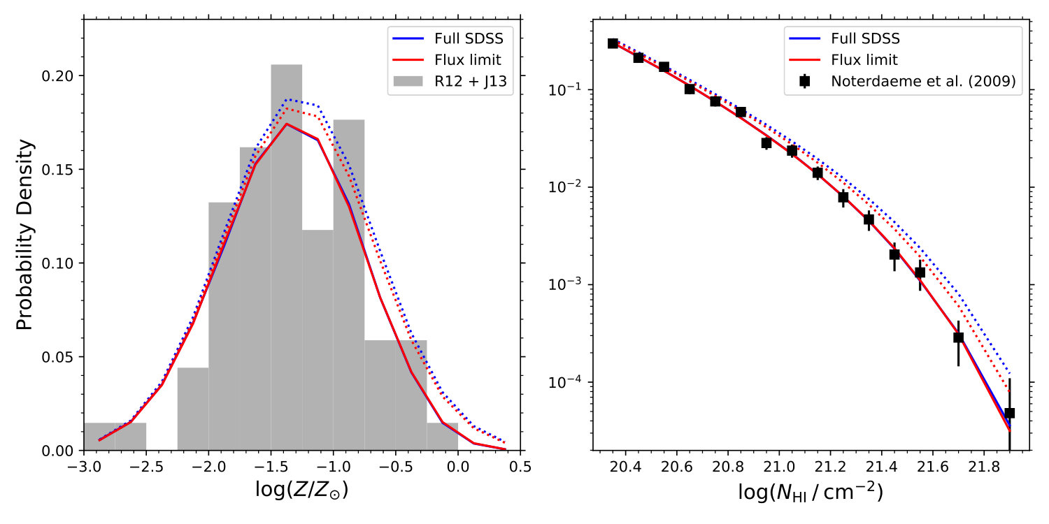 Figure 1
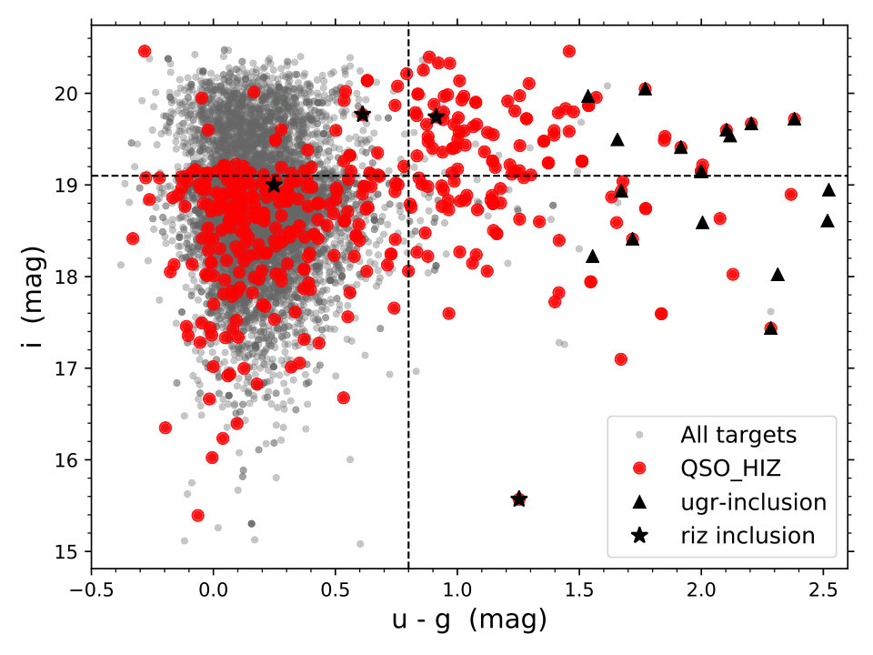 Figure 2
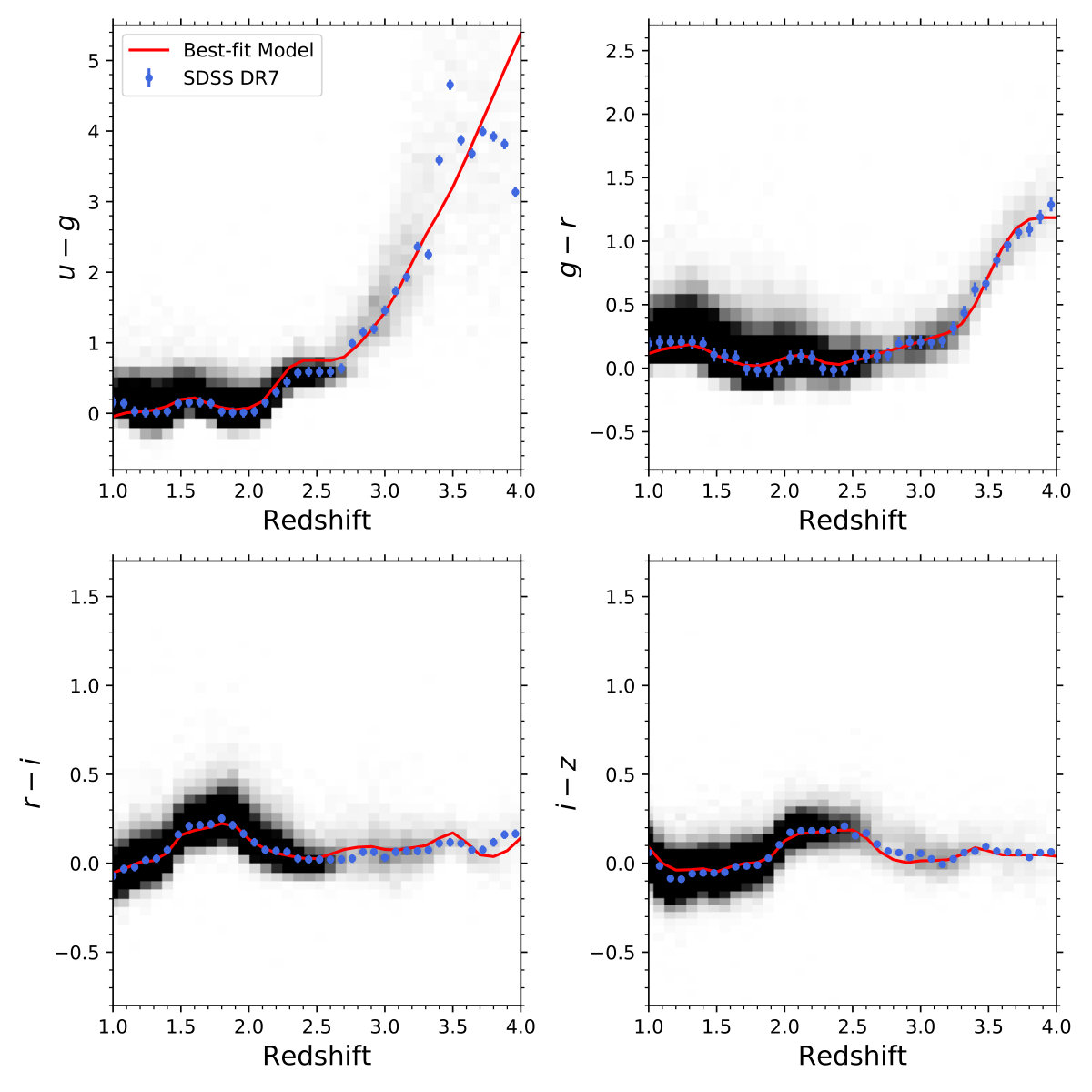 Figure 3
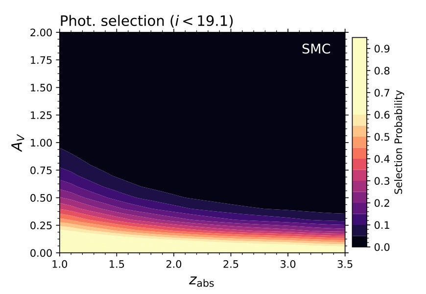 Figure 4
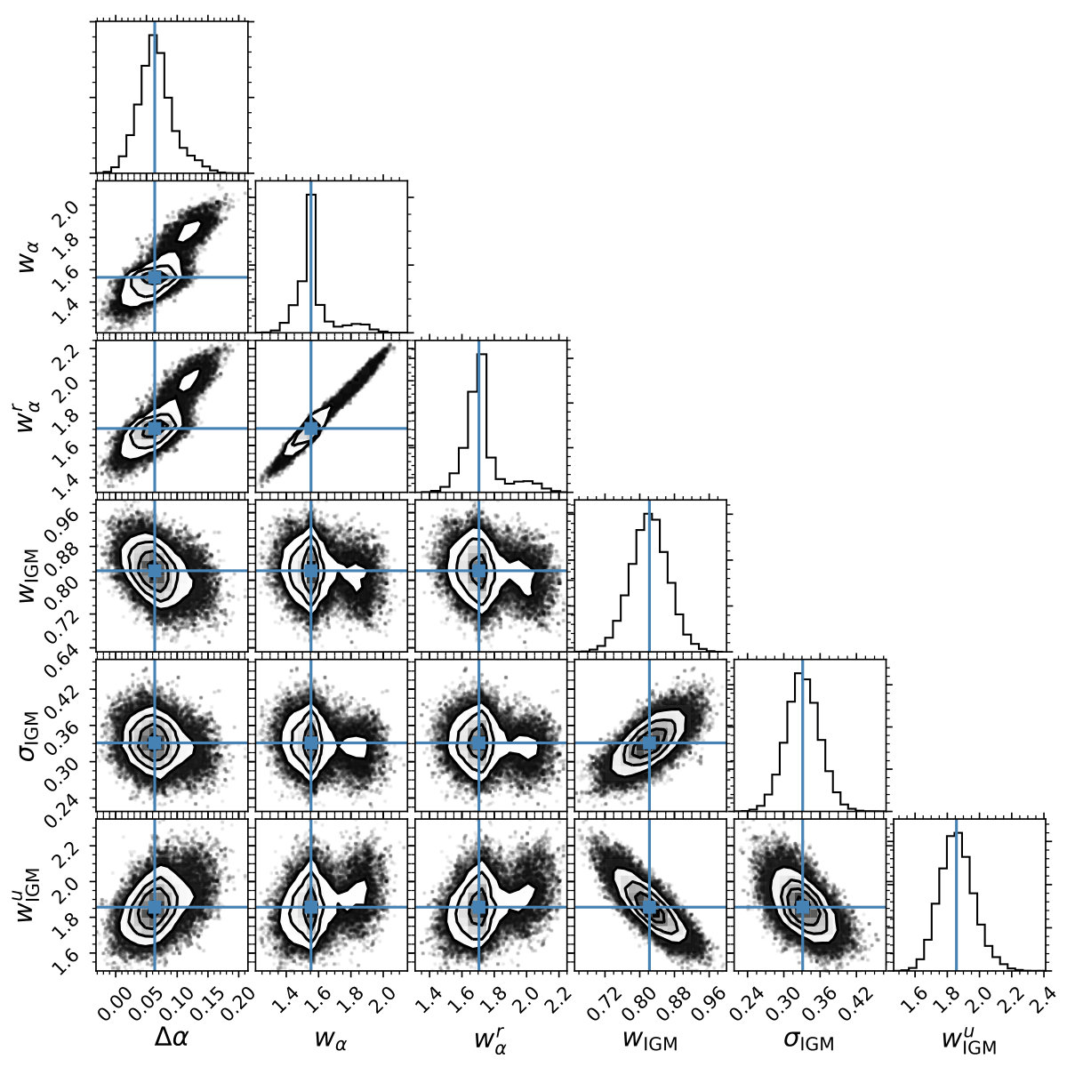 Figure 5
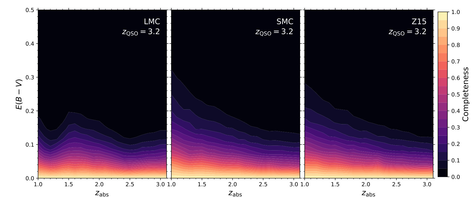 Figure 6
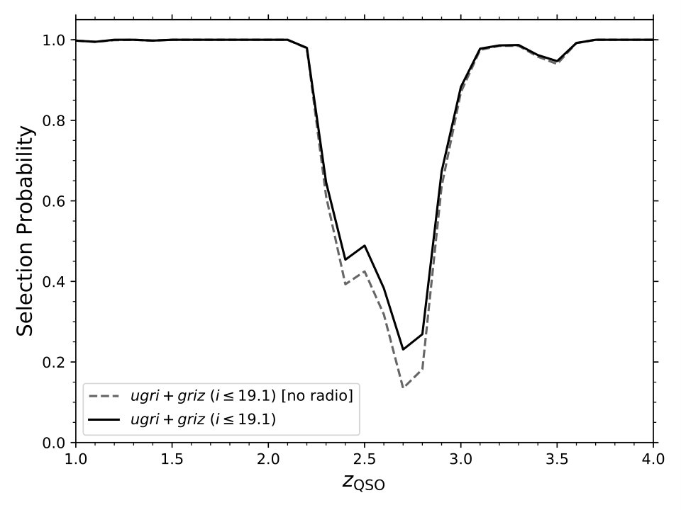 Figure 7
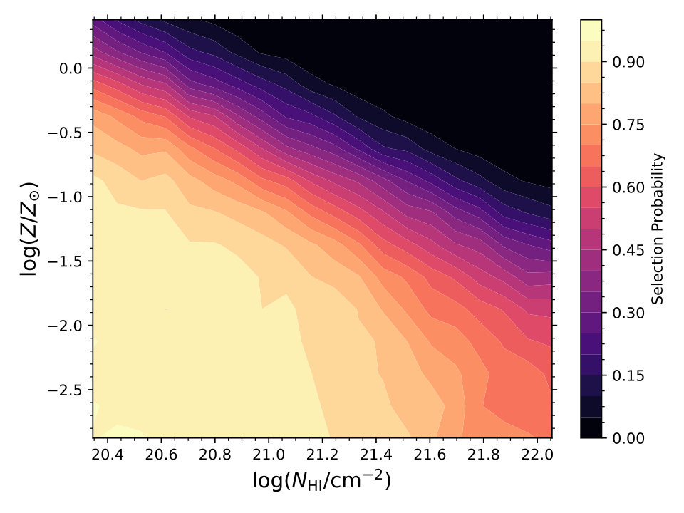 Figure 8
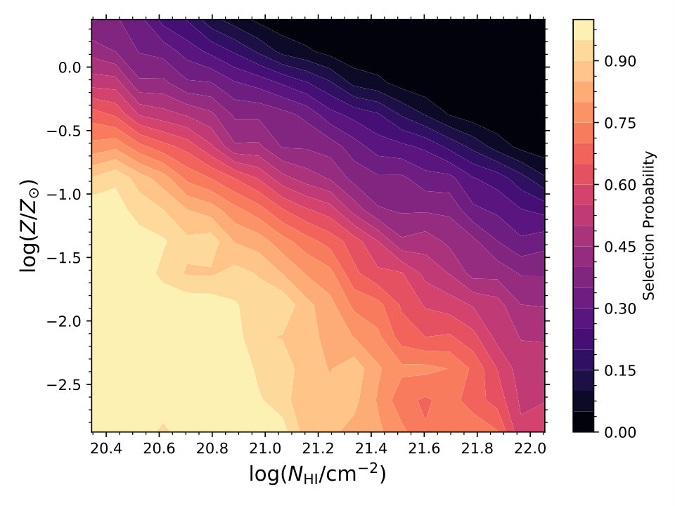 Figure 9
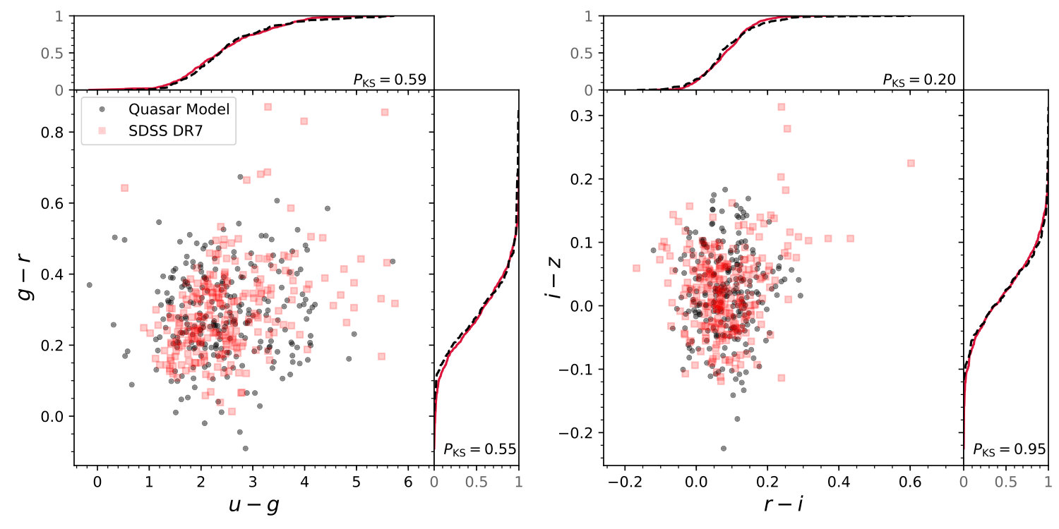 Figure 10
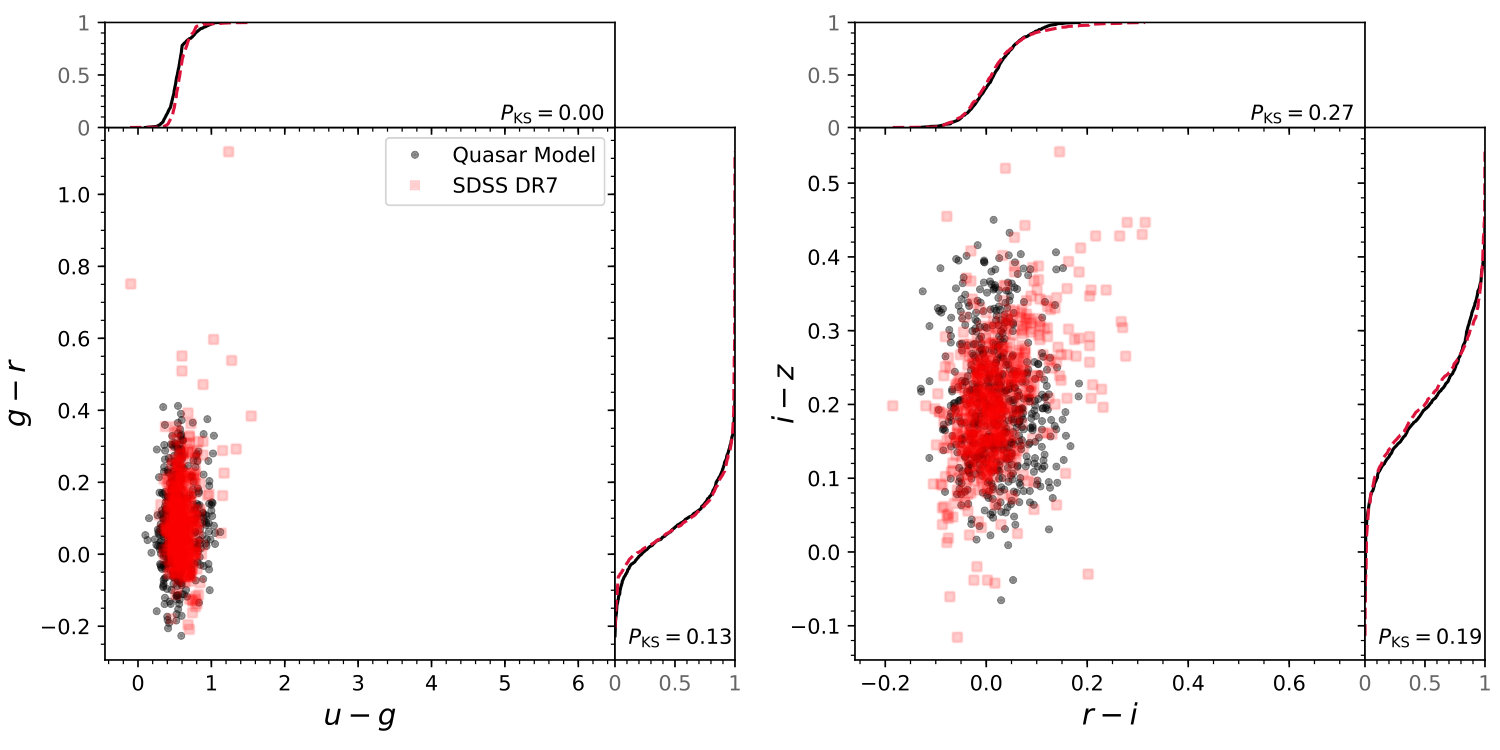 Figure 11
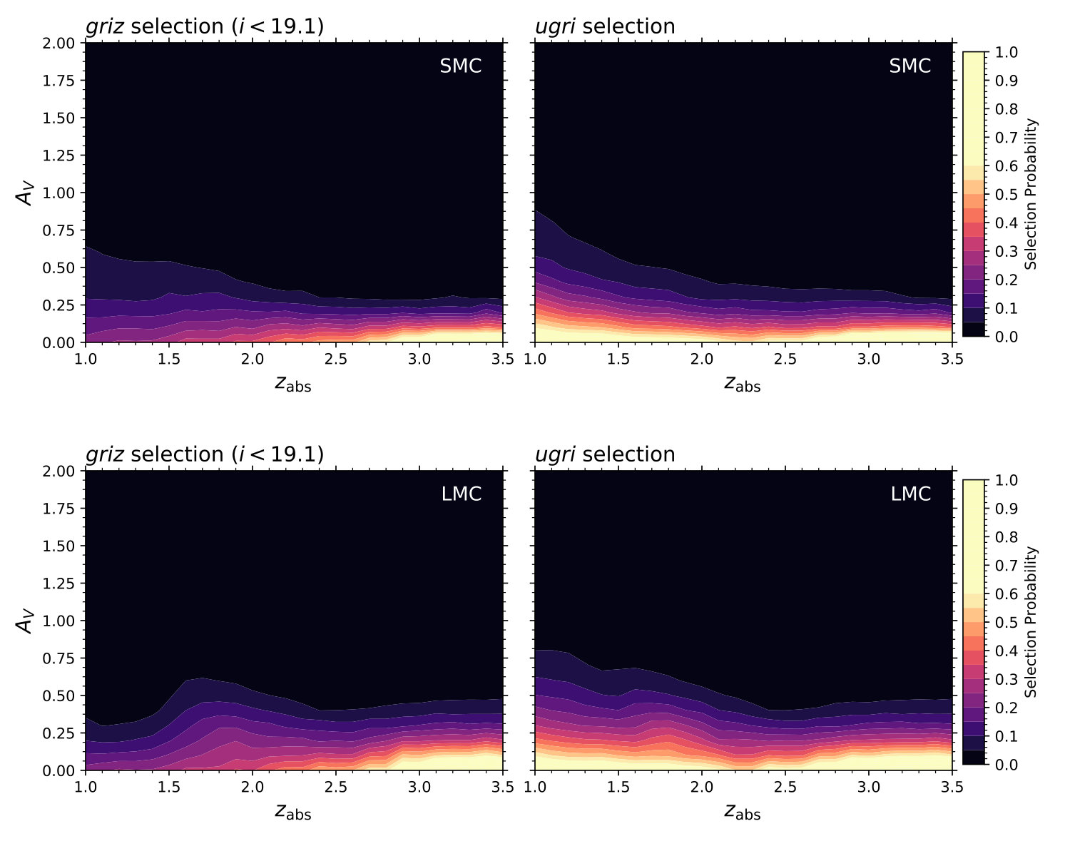 Figure 12
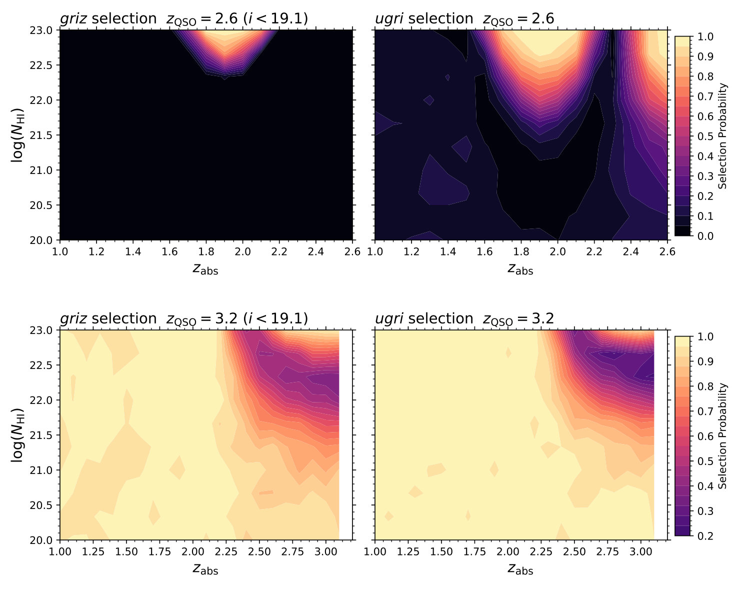 Figure 13
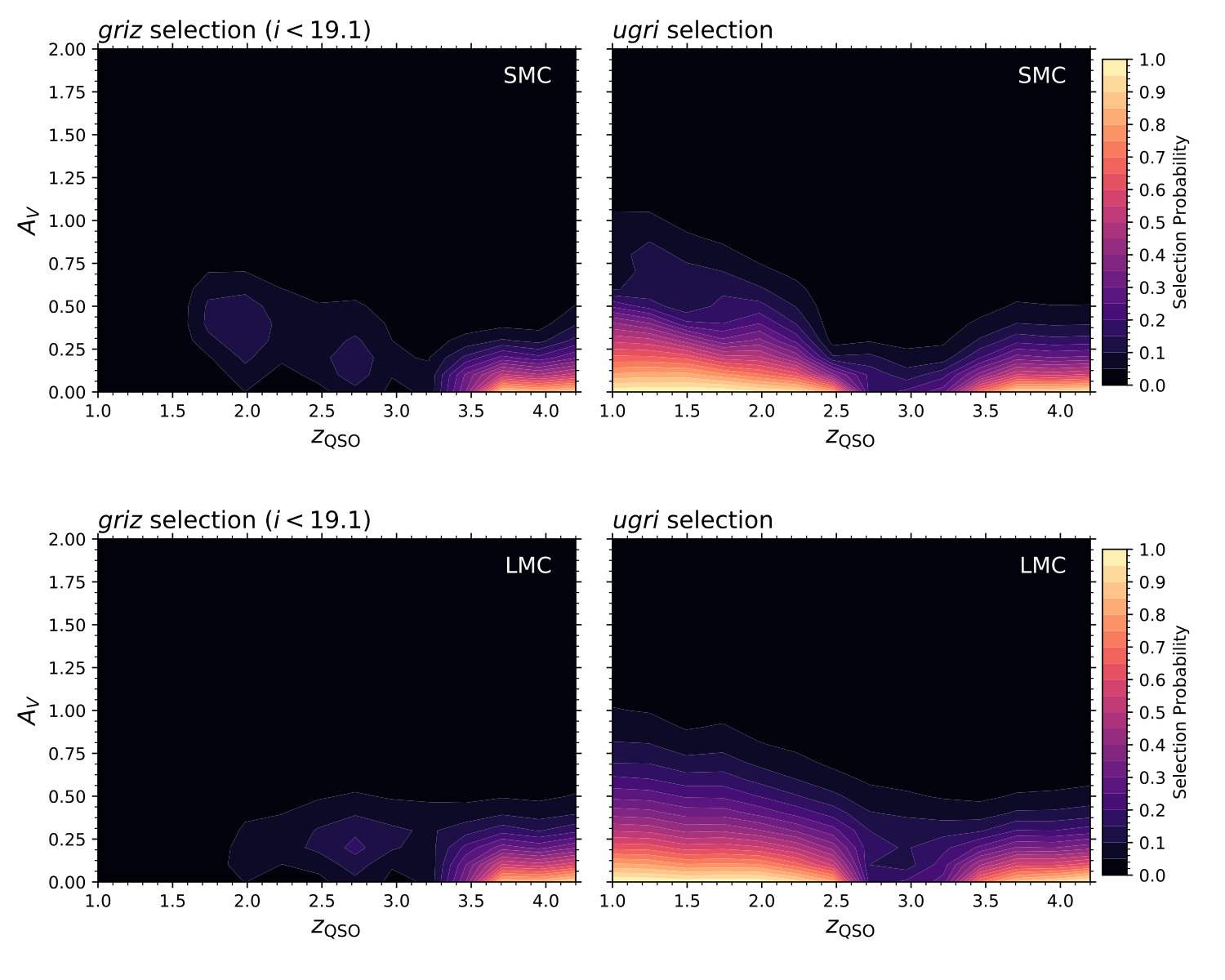 Figure 14
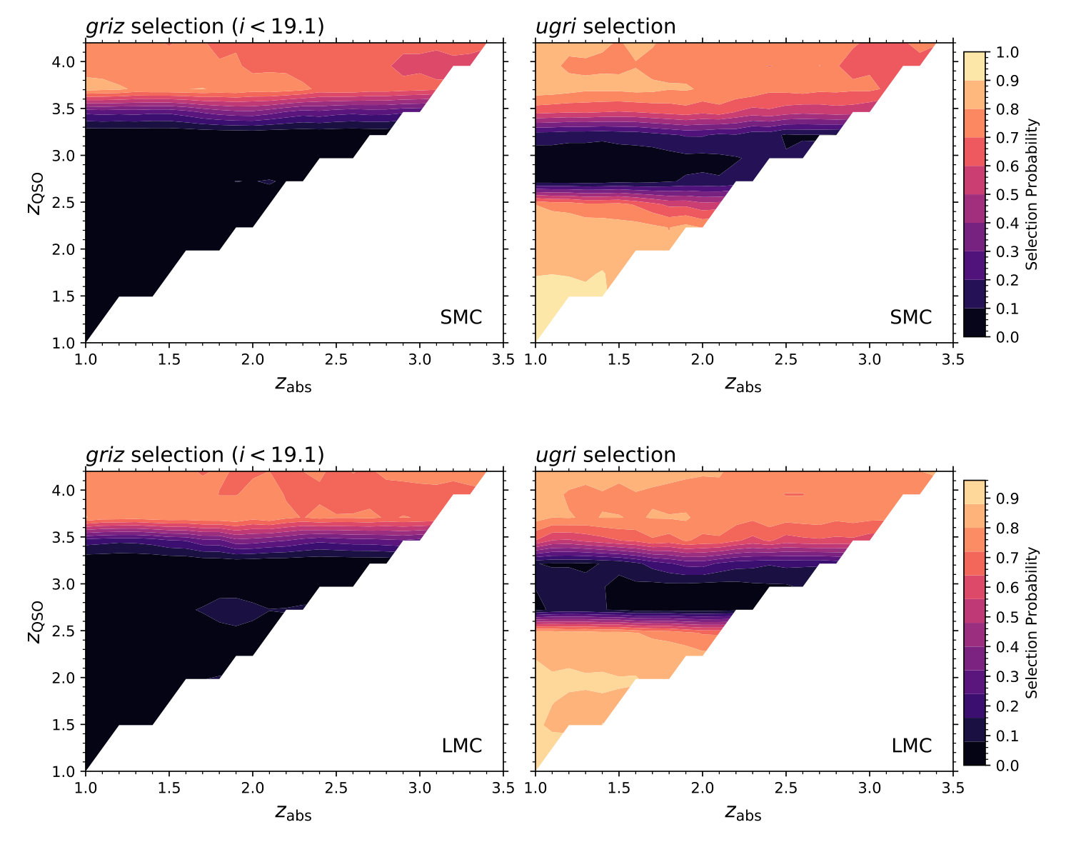 Figure 15
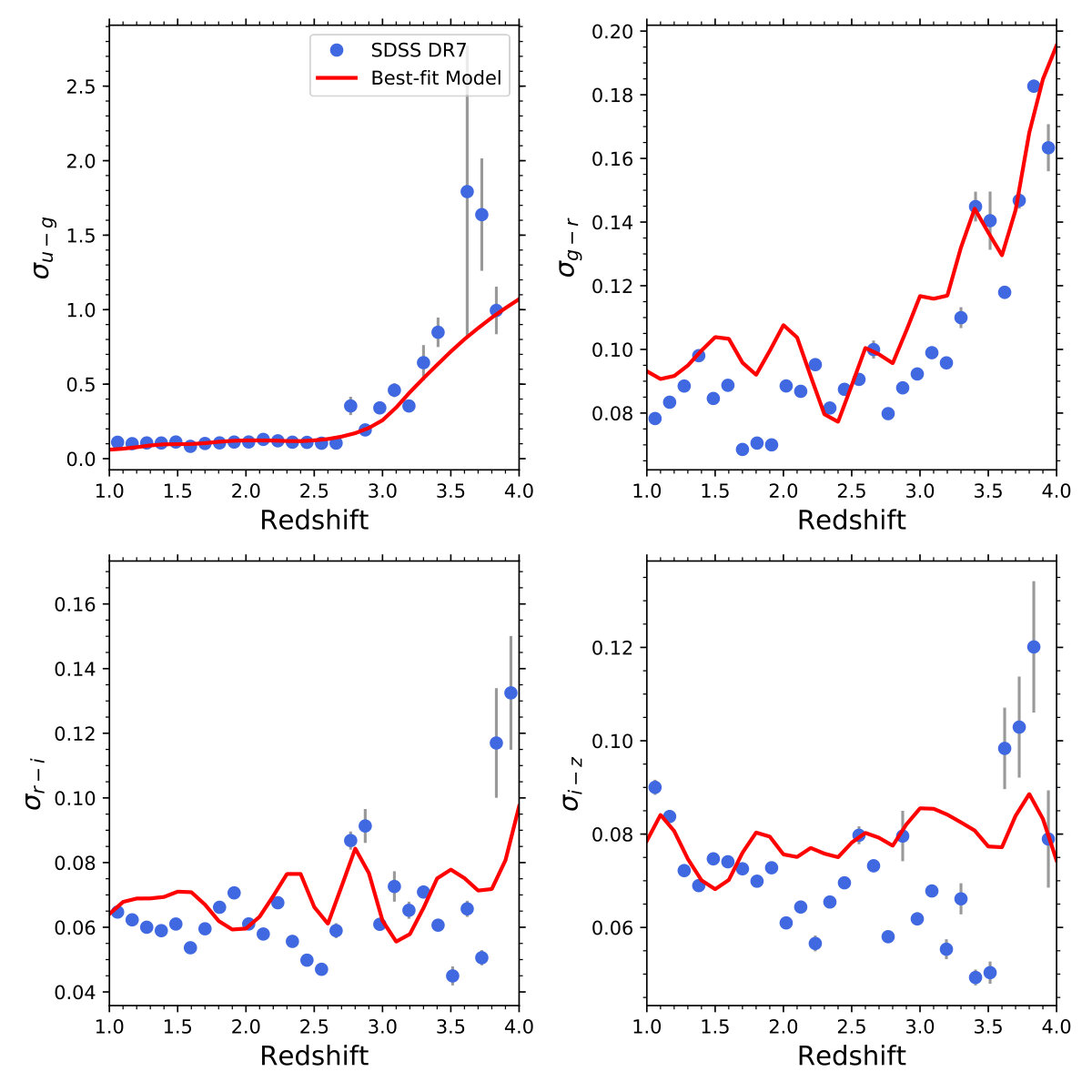 Figure 16
| / mmag | |||||||
|---|---|---|---|---|---|---|---|
| / mmag |
| / mmag | |||
|---|---|---|---|
| / mmag |
| Model | PP09 | ||
|---|---|---|---|
| / mmag | |||
| / mmag |
| Parameter | = | |
|---|---|---|
| Model | l99 | u99 |
|---|---|---|
| / mmag | ||
| / mmag |
| Model | l99 | u99 |
|---|---|---|
| / mmag | ||
| / mmag |
Peer Reviews
No public reviews on file for this paper yet. If you reviewed it on a platform where reviews are public (OpenReview, ICLR, NeurIPS, ICML), you can paste yours below so the community can read it here.
Videos
No videos yet. Explain this paper in a talk, walkthrough, or lecture? Add one.
The effect of dust bias on the census of neutral gas and metals in the high-redshift Universe due to SDSS-II quasar colour selection
Jens-Kristian Krogager1, Johan P. U. Fynbo2,3, Palle Møller4, Pasquier Noterdaeme1,Kasper E. Heintz5,3 and Max Pettini6
1Institut d’Astrophysique de Paris, CNRS-SU, UMR7095, 98bis bd Arago, 75014 Paris, France
2Dark Cosmology Centre, Niels Bohr Institute, University of Copenhagen, Juliane Maries Vej 30, 2100 Copenhagen Ø, Denmark
3The Cosmic Dawn Center, Niels Bohr Institute, University of Copenhagen, Juliane Maries Vej 30, 2100 Copenhagen Ø, Denmark
4European Southern Observatory, Karl-Schwarzschildstrasse 2, 85748 Garching bei München, Germany
5Centre for Astrophysics and Cosmology, Science Institute, University of Iceland, Dunhagi 5, 107 Reykjavík, Iceland
6Institute of Astronomy, Kavli Institute for Cosmology, Madingley Road, Cambridge CB3 0HA, United Kingdom
Abstract
We present a systematic study of the impact of a dust bias on samples of damped Lyman- absorbers (DLAs). This bias arises as an effect of the magnitude and colour criteria utilized in the Sloan Digital Sky Survey (SDSS) quasar target selection up until data release 7 (DR7). The bias has previously been quantified assuming only a contribution from the dust obscuration. In this work, we apply the full set of magnitude and colour criteria used up until SDSS DR7 in order to quantify the full impact of dust biasing against dusty and metal-rich DLAs. We apply the quasar target selection algorithm on a modelled population of intrinsic colours, and by exploring the parameter space consisting of redshift, (and ), optical extinction, and H i column density, we demonstrate how the selection probability depends on these variables. We quantify the dust bias on the following properties derived for DLAs at : the incidence rate, the mass density of neutral hydrogen and metals, the average metallicity. We find that all quantities are significantly affected. When considering all uncertainties, the mass density of neutral hydrogen is underestimated by 10 to 50%, and the mass density in metals is underestimated by 30 to 200%. Lastly, we find that the bias depends on redshift. At redshift , the mass density of neutral hydrogen and metals might be underestimated by up to a factor of 2 and 5, respectively. Characterizing such a bias is crucial in order to accurately interpret and model the properties and metallicity evolution of absorption-selected galaxies.
keywords:
galaxies: high-redshift — quasars: absorption lines — cosmology: observations
††pagerange: The effect of dust bias on the census of neutral gas and metals in the high-redshift Universe due to SDSS-II quasar colour selection–LABEL:lastpage
1 Introduction
Quasar absorption systems are invaluable tools for our understanding of neutral gas at high redshift, as this is currently the only way to study the neutral gas phases beyond the local environment where emission studies are sensitive. One such class of quasar absorption systems, the so-called damped absorbers (DLAs), are of particular importance since the high column density of H i ( cm*-2*, Wolfe et al. 1986) ensures that the hydrogen is predominantly neutral. Due to the low fraction of ionized gas in DLAs, we can infer very precise measurements of the abundances of metal species. Moreover, the neutral gas mass density in the Universe is dominated by these high column density systems (Lanzetta et al., 1995; Prochaska et al., 2005; Noterdaeme et al., 2009b). Since the neutral gas phase is needed in order to form molecules and subsequently stars, DLAs therefore provide important clues about the gas reservoir from which stars form over most of cosmic time.
Since certain elements (e.g., Fe, Cr, Mn) tend to deplete strongly into dust grains, their gas-phase abundances (as measured from absorption lines) are lowered according to the strength of the depletion. By studying abundance ratios in DLAs it is therefore possible to conclude that some amount of dust must be present in most DLAs (e.g., Ledoux et al., 2003; De Cia et al., 2016). Moreover it is found that the optical extinction, , scales with and metallicity (Vladilo & Péroux, 2005; Zafar & Watson, 2013). The more metal-rich and high-column density systems will therefore have a higher dust opacity. This will lead to a bias against metal-rich and high systems as these are more likely to be missed in optically selected, flux-limited surveys (Pei et al., 1991). The effect of obscuration has been studied statistically throughout the last decades, reaching conflicting conclusions about the average reddening from DLAs. Most studies agree that the average reddening is low but measurements still present a rather large scatter ranging from around 0.002 to 0.01 mag, with the strength of the effect varying from weak to no bias in optically selected DLA samples (e.g., Pei et al., 1991; Murphy & Liske, 2004; Vladilo et al., 2008; Pontzen & Pettini, 2009; Frank & Péroux, 2010; Kaplan et al., 2010; Khare et al., 2012). Alternatively, by selecting quasars purely based on their radio properties, the effect of a dust bias can be largely overcome as electromagnetic radiation at radio wavelengths does not suffer from dust obscuration (Ellison et al., 2001; Jorgenson et al., 2006). Yet, an optical counterpart must still be detectable to spectroscopically confirm the source as being a quasar. The largest analysis of radio selected quasars has put an upper limit on the average reddening from DLAs of mag (Ellison et al., 2005). However, the study is limited by the small sample size of only 14 DLAs from a total of 42 radio-selected quasars with optical and near-infrared data available. Combining optical and radio constraints, Pontzen & Pettini (2009) estimate that a small fraction of absorbers (less than around 5%) will be missed due to dust obscuration, but that the mass density of metals, , might be underestimated by up to a factor of two. Recently, Murphy & Bernet (2016) reanalysed the quasar sample of the Sloan Digital Sky Survey (York et al., 2000, SDSS) data release 7 (DR7). The authors find a low average reddening of mag and conclude that the optical criteria (both in terms of flux and colours) used for target selection in SDSS prior to DR7 have a negligible effect on their estimated reddening. While the authors replicate the complex selection function of SDSS DR7 to support their conclusion, they do not provide a full analysis of the impact of the selection effects on the observed metallicity and distributions.
While the number of systems missed due to a dust bias might be small (less than 5% in number, Pontzen & Pettini 2009), these systems are preferentially metal-rich and dusty and thus more likely to harbour cold neutral gas and molecules (Ledoux et al., 2003; Srianand et al., 2005, 2008; Noterdaeme et al., 2009a; Noterdaeme et al., 2018). It is therefore important to quantify the full implications of dust reddening and obscuration for our understanding of the cold ( K), dust-rich gas phases in DLAs. In an attempt to identify this obscured population of dusty DLAs, we have applied optical and near-infrared photometric criteria to observe reddened quasars that are not targeted by the SDSS selection algorithm (Fynbo et al., 2013; Krogager et al., 2015, 2016b). Based on these tailored surveys, we have identified three dusty DLAs at high redshift () towards quasars that were not flagged as quasar candidates in SDSS (Krogager et al., 2016a; Fynbo et al., 2017; Heintz et al., 2018b). All of these absorbers have high metallicity, and while cold ( K), neutral gas is only securely detected in the absorber HAQ2225+0527 (Krogager et al., 2016a), it is highly probable that higher resolution spectroscopy of the remaining DLAs will reveal similarly cold, neutral gas.
In this work, we study the combined effects of dust obscuration and reddening on the quasar selection in SDSS DR7 (Richards et al., 2002). In order to assess the selection probability of quasars, we first simulate intrinsic quasar colours and magnitudes as a function of redshift. We then introduce various absorber properties in front of the intrinsic quasar photometry and replicate the SDSS selection algorithm in order to quantify the effect of various parameters. Following the analysis of Pontzen & Pettini (2009), we use our calculated selection probabilities to infer the intrinsic distribution functions for metallicity and , and find that the full, combined optical selection (using both colour and flux-limit) leads to a significantly stronger bias than assuming a flux-limit alone. This is somewhat alleviated if assuming that a small fraction of quasars are selected irrespective of their optical properties (similar to the cross-matching to radio sources performed in the SDSS). We stress that all references to SDSS throughout this work refers solely to the first epochs of SDSS (I and II up until data release 7) before the onset of the Baryon Oscillation Spectroscopic Survey (BOSS, also referred to as SDSS-III), since the spectroscopic target selection changed completely from the algorithm described in Richards et al. (2002) for SDSS I/II to the more complex algorithms used for BOSS (Richards et al., 2009; Yèche et al., 2010; Kirkpatrick et al., 2011; Bovy et al., 2011; Ross et al., 2012). While the spectroscopic target selection for quasars is more complex for the BOSS sample, the selection is still based on optical information and is therefore still susceptible to biases. Moreover, the average reddening effect by DLAs has only been studied for DLAs selected from the quasar sample of SDSS data-release 7 (DR7). We therefore do not consider the quasar samples of later data-releases in the current work. The effect of the BOSS quasar selection will be studied in a forthcoming paper.
This paper is organized as follows: In Sect. 2, we describe our simulated photometry and the calculation of selection probabilities; In Sect. 3, we present our calculation of fractional completeness of absorption-derived quantities such as the gas mass density of neutral gas and metals in DLAs; The systematic uncertainties related to our modelling are investigated in Sect. 4; In Sect. 5, we discuss the results and implications of our work as well as the related caveats, and lastly in Sect. 6, we summarize our results.
Throughout this work, we will assume a flat CDM cosmology with , and (Planck Collaboration 2014).
2 Quasar Colour Selection
We investigate the effect of dust reddening by replicating the colour and magnitude selection algorithm of SDSS. As input to the selection algorithm, we simulate an intrinsic population of quasars at different redshifts () with varying amounts of foreground dust () at various absorption redshifts () for two broad classes of extinction laws (SMC and LMC; as quantified by Gordon et al. 2003). Moreover, we include the reddening effect of strong H i absorption in our model. In the following section, we will describe the details of how we simulate the intrinsic quasar properties, how we apply the SDSS quasar selection algorithm, and how we simulate the absorption properties and calculate the selection probabilities. Using a physically motivated model in which metallicity () and scale with , we then calculate the selection probabilities as a function of and . We use this 2-dimensional selection probability to fit intrinsic distributions of and in order to reproduce the observed distributions of by Rafelski et al. (2012) and Jorgenson et al. (2013) and of by Noterdaeme et al. (2009b) as well as the observed average reddening measured by Murphy & Bernet (2016). Lastly, we calculate the fractional completeness in various observable quantities for DLAs following Pontzen & Pettini (2009).
2.1 Constructing the Statistical Samples
In order to make a meaningful statistical comparison between our model and the data, we only consider quasars brighter than the magnitude-limit used for the complete sample of quasars in SDSS (). The quasar sample of SDSS does include a significant number of targets fainter than this limit, but the completeness is low ( % for based on the luminosity function at this redshift). It is therefore not possible for us to replicate this deeper selection (referred to as ‘high- quasar selection’ or ‘’-selection, see Sect. 2.3) in a statistically meaningful way.
Since the data by Rafelski et al. (2012), Noterdaeme et al. (2009b) and Murphy & Bernet (2016) are based on the full sample of DLAs in SDSS up until data-release 7 (DR7) irrespective of the brightness of the background quasar, we first have to clean the samples and remove DLAs observed towards quasars that do not meet the -band flux-limit. The sample by Rafelski et al. (2012) is composed of a purely SDSS-selected sub-sample from DR5 (their table 2) together with a sample compiled from the literature (their table 3). Since a large part of the literature sample is not covered by the SDSS foot-print, we are not able to obtain SDSS -band magnitudes. Instead, we have used available -band photometry from the Pan-STARRS1 (Chambers et al., 2016) as this survey uses a very similar -band to that of SDSS. When no photometry is available from neither SDSS nor Pan-STARRS1, we have used available broad-band photometry in , , and bands to infer an -band magnitude based on colour transformations between the various magnitude systems. In those cases, the targets are several magnitudes brighter than the limit, and the large uncertainty in the colour transformations is therefore not important. For one target (J02422917) we have not been able to obtain any photometric information. This object has been excluded from the final sample. Based on the photometry, we discard all DLAs for which the background quasar is fainter than . Moreover, we exclude targets where the metallicity is based on a combination of limits or on refractory elements alone (Fe, Ni, Cr, etc.).
We furthermore include the DLA sample of metallicities by Jorgenson et al. (2013) homogeneously selected from SDSS DR5 with . However, we remove duplicates between the two samples giving preference to measurements based on sulphur over those based on silicon and similarly we give preference to higher resolution measurements. As for the ‘Rafelski sample’, we remove measurements based on refractory elements or limits. This results in a total sample of 202 DLAs with good quality metallicity measurements.
We highlight that the quasar selection algorithm did not change up until DR7 and hence all SDSS data-releases before and including DR7 are based on the selection algorithm as presented by Richards et al. (2002). The literature sample included by Rafelski et al. (2012) is not strictly selected based on the same criteria as the SDSS selection algorithm; however, since quasars before SDSS were mainly identified either via radio observations or the UV excess method, both of which are explicitly included in the SDSS algorithm, we argue that the literature sample of Rafelski et al. would very likely have been targeted by the SDSS selection algorithm that we study in this work. This claim is further bolstered by the fact that such ‘pre-SDSS’ quasars were incorporated in the sample of quasars used to optimize the SDSS algorithm (Richards et al., 2002).
The samples by Noterdaeme et al. (2009b) and Murphy & Bernet (2016) are derived purely from SDSS-DR7 and we can therefore easily clean out the DLAs in front of quasars fainter than . The average reddening measurement by Murphy & Bernet (2016) is mmag. We find a consistent average reddening for the flux-limited sub-sample yet with a slightly larger uncertainty: mmag.
Similarly, we find no effect on the distribution function derived by Noterdaeme et al. (2009b) when restricting the sample to quasars with .
2.2 Simulating Quasar Photometry
In order to generate proper input for the SDSS quasar selection algorithm, we need not only the colour information but also the magnitudes in the 5 filters of SDSS (, , , , and ). We therefore draw samples from the quasar luminosity function as a function of quasar redshift (Manti et al., 2017) down to a limiting magnitude of . To get the right distribution of colours we construct a fiducial quasar model based on available constraints from the literature. For this purpose, we use the quasar template by Selsing et al. (2016) as a basis for the spectral energy distribution; however, as the template only covers rest-frame wavelengths down to 1000 Å, we extend the template bluewards of Å by assuming a power-law with a spectral index of (Lusso et al., 2015). This break wavelength corresponds fairly well to the break in the power-law spectral shape observed by Lusso et al. (2015), who infer Å. The template is redshifted to the given and scaled to the absolute flux as determined from the luminosity function. This results in a 5-element vector of magnitudes per band denoted referring to the -th random realisation of quasar photometry drawn from the luminosity function.
Since the intrinsic properties of quasars are known to vary from object to object, we include variations in the intrinsic power-law spectrum. The change in power-law index is applied as a relative offset () with respect to the intrinsic value of (Selsing et al., 2016). For the fiducial model, has a value of [math]. Following Krawczyk et al. (2015), we assume that the power-law index is distributed as a Gaussian centred at the intrinsic value of the template with a width of . Rather than randomly assigning a value of the power-law index for each realisation, we calculate the offset in magnitudes per band as a function of redshift relative to the intrinsic template for a change of in power-law index. This allows us to evaluate the mean colors at a given redshfit without having to evaluate a large ensemble. The pre-evaluated offsets per band is denoted as the 5-element vector, . For each quasar realisation, we then draw a random number from a Normal distribution and multiply by . Lastly, in order to take into account variations of emission lines, we scale by the parameter , which for the fiducial model has the value .
The last effect we include in the fiducial model is the attenuation bluewards of the quasar emission line due to hydrogen Lyman-series absorption from the intergalactic medium. We use the theoretically derived average attenuation for different redshifts as a function of wavelength by Meiksin (2006) to calculate the redshift-dependent average attenuation per band denoted 111The average attenuation is calculated by interpolating between the values given by Meiksin (2006).. The attenuation is assigned a randomly drawn weight from a Normal distribution: , where is an overall normalization of the theoretical prediction in order to match the data, and determines the dispersion in IGM absorption from one object to another. This mimics effects of random sight lines through the forest. For the fiducial model, the parameters of this distribution are: .
The final 5-band photometry for a given realisation, , is then calculated as:
[TABLE]
For each of the realizations of quasar magnitudes in the 5 SDSS filters, we assign photometric uncertainties following an empirically derived model between magnitude and uncertainty inferred from point source data in SDSS DR7. We fit the distribution of photometric uncertainties as a function of observed magnitudes for each of the five bands using a 4th order polynomial. For sources with magnitudes larger than mag, we assign a constant photometric uncertainty. This does not significantly affect our simulations, as targets this faint will not meet the -band criterion and hence will not be considered for target selection. Following Richards et al. (2002), we increase the photometric uncertainties by 0.0075 mag (added in quadrature) to account for systematic uncertainties in the flux calibration. The authors moreover add an error contribution from the correction for Galactic extinction, for which they add in quadrature 15% of the extinction value to the photometric uncertainty. Since we do not simulate the projected sky position of our targets, we simply assume a median correction in the five filters of for , , , , , respectively. The median Galactic correction values are derived from 10 000 quasars in SDSS DR7. We then add in quadrature 15% of the median for each filter to the uncertainty of the given filter.
In order to optimize this fiducial model, we fit the 4 colour relations of the SDSS colour-space (, , , ) as a function of redshift. We parametrize the colour–redshift relations by measuring the ‘mode’ and standard deviation of the 4 colour distributions in redshift bins of . In order to reproduce the mode of the observed colour–redshift distribution, we only need to vary the parameters: and . The widths of the distributions are not fitted during the same process, since they do not alter the mode of the distributions. We will instead constrain the width of the distributions in a subsequent step. We note that we fit the mode of the observed distributions since this quantity will be less affected by dust reddening compared to the mean and the median of the colour distributions. The best-fit model parameters are and ; However, we find that in order to fit the colour properly we need to increase the IGM absorption in the -band by a factor . The resulting colour–redshift relations are shown in Fig. 1.
In order to constrain the parameters and , we fit the width of the colour–redshift distributions while keeping the parameters and fixed to their best-fit values. In Fig. 2, we show the model for the best-fit parameters and . Although we include uncertainties in Fig. 2, these are not taken into account in the fit, since this would give much stronger weight to the low-redshift bins where there are many more quasars. In order to give equal weight to all redshifts during the fit, we use an average uncertainty of 0.01 for all measurements.
The intrinsic properties of the simulated data match well the observed properties of spectroscopically confirmed quasars as shown in Figs. 1 and 2. This allows us to probe the overall redshift dependence of the quasar selection algorithm (see Sect. 2.3). Yet, there are still significant discrepancies for certain redshift intervals. While it is beyond the scope of the current work to reproduce in detail the quasar properties over the full redshift range, we do attempt to optimize the model in certain redshift ranges of interest. Specifically for quasars at and , which we use for the detailed analysis of dust bias against absorption systems in Sect. 3, we optimize the quasar model. The additional optimization and robust evaluation of model uncertainties are described in Appendix A.
In the quasar model described above, we have neglected the contribution of BAL quasars as these are anyways not included in the sample of quasars used for absorption analyses. Other possible effects that could affect our intrinsic quasar photometry model would be systematic variations in the emission lines, e.g., the Baldwin effect (Baldwin, 1977), blazars with no apparent emission lines, or quasars with abnormal spectral shapes (Meusinger et al., 2012). However, as blazars and quasars with abnormal spectral shapes contribute very little to the overall population of quasars (Meusinger et al., 2012; Li et al., 2015), we have neglected the contribution of these in order to keep the model as simple as possible.
2.3 SDSS quasar candidate selection
The simulated photometry and errors described above are then passed through the steps of the selection algorithm as outlined in figure 1 of Richards et al. (2002). The calculation is split into two selection ‘branches’: , selected in the 3-dimensional , , and colour space, and , selected in the 3-dimensional , , colour space. We have re-implemented the definition of the ‘stellar locus’ in and colour-spaces by Richards et al. (2002). The details of our new implementation in Python are given in Appendix C. Since we are working on simulated photometry, we do not implement the checks for photometric data quality flags. Moreover, these photometric impurities will not introduce any significant bias but merely lower the completeness. Lastly, we apply the same magnitude cut as Richards et al. (2002), namely, mag and mag for targets in the and colour-spaces, respectively. However, for our statistical analysis, we use a single magnitude cut of . The resulting fraction of simulated quasars identified through the algorithm will hereafter be referred to as the selection probability, .
Since we only consider quasars brighter than for the statistical bias calculation in this work, the total selection probability is then given by the union of the two selection branches, and simultaneously fulfilling the -band criterion:
[TABLE]
where denotes the number of quasars that are selected either by the or criteria.
Lastly, we implement a mock radio selection corresponding to the cross-matching between FIRST (Becker et al., 1995) and SDSS by simply allowing a constant fraction of quasars to be selected irrespective of their optical colours. Here we assume a fraction of radio detections of 10% inferred from FIRST cross-matching in independent surveys (Hewett et al., 2001; Krogager et al., 2016b). Thus, 10% of the simulated quasars will be allowed to pass the quasar selection irrespective of the colour criteria; Nevertheless, the quasars still have to pass the -band magnitude limit. The result of passing the intrinsic quasar photometry as described in Sect. 2.2 is shown in Fig. 3. We recover the strong drop in selection probability for quasars with redshift as demonstrated in the original work by Richards et al. (2002). This low sensitivity for quasars in this redshift range is caused by the fact that the quasar colours cross the stellar locus in the optical colour spaces utilized by the SDSS. For the redshift range , we have carried out a similar optimization of the quasar model as described in Appendix A.
2.4 Absorption Properties
We here investigate the effect of applying intervening dust reddening and strong H i absorption to the quasar photometry. In the first part, we will simply calculate the selection probability for the various parameters in order to visualize the dependence of the selection probability on these variables. We therefore sample all properties uniformly and calculate the selection probability in this parameter space. In the second part, we will use a physically motivated model to calculate how the selection probability affects the observed distributions of metallicity and column density of H i.
When simulating the absorber properties, we set up a grid of quasar redshifts in the interval (in steps of 0.2), with absorber redshifts in the range in steps of 0.1 and requiring that , with in the interval mag in steps of 0.1, and with in the range in steps of 0.3. For each point in this 4-dimensional parameter space (, , , ), we then simulate an ensemble of 1000 quasars as described in Sect. 2.2 and apply the properties and to the simulated quasar photometry. The ensemble is then passed through the SDSS quasar selection algorithm and the selection probability is calculated. We perform this calculation twice assuming different reddening laws: either SMC- or LMC-type as parametrized by Gordon et al. (2003).
In Fig. 4, we show the resulting and in the (, )-grid averaged over all quasar redshifts and all values of . For comparison, we show the selection probabilities of quasars for a purely flux limited selection of . These flux-limited-only calculations were performed on the same simulated data simply by skipping the colour selection criteria and only applying the -band magnitude cut. In Appendix B, we show the averaged and in the (, ) and (, ) parameter spaces respectively.
In the above analysis, we have not assumed any physical relation between absorber properties and , however, it is well known that scales with both and metallicity (Vladilo & Péroux, 2005; Zafar & Watson, 2013, e.g.,). We therefore run a similar set of models as described above assuming a fixed dust-to-metals ratio () to investigate the effect of the colour selection on the and distribution of absorbers. We use the relation by Zafar & Watson (2013) to quantify the -band dust extinction in terms of and :
[TABLE]
where is the dust-to-metal ratio.
In order to compare our results to the previous work by Pontzen & Pettini (2009), we will assume an absorption redshift of which corresponds to the median redshift of absorbers in the analysis by Pontzen & Pettini (2009). While Pontzen & Pettini (2009) do not worry about the redshift of the background quasar, we must take this into account when estimating the bias of the full SDSS selection criteria, since the colours depend on . In the following, we assume that the background quasars are at an average . We will also investigate the selection probability at lower redshift () to demonstrate the redshift dependence of the bias.
We evaluate the selection probability at the specific redshift as a function of and , denoted , in the ranges of and , by uniformly drawing 200 000 sets of and . For each draw, we randomly assign a realization of intrinsic quasar photometry in the five SDSS bands for the given following the same method as described in Sect. 2.2. The optical extinction is then calculated using eq. (3), and the quasar fluxes are attenuated according to the SMC extinction law applied in the absorber rest-frame. Here we only focus on the SMC extinction curve as this the most commonly observed type of extinction for DLAs (see also Sect. 5.2). Furthermore, we apply the extinction from the DLA absorption itself. As before, the quasar photometry is passed through the selection algorithm and the selection probability in the 2-dimensional (, )-space is calculated. In Fig. 5, we show the selection probability for two models of and , and and . Both models are calculated assuming a value of for the SMC extinction law. It is clearly seen that the selection probability drops for high metallicity and high due to the increasing reddening moving diagonally from the bottom left corner to the top right corner.
3 Dust Bias in Damped Absorbers
We are now able to use the inferred selection probability, , to infer the completeness in metallicity and distributions of DLAs at . Since the colour selection is very redshift dependent, we also perform a calculation of the completeness for lower redshift DLAs at towards quasars at where the SDSS selection algorithm is very inefficient. For this purpose, we assume analytic, parametric functional forms for the intrinsic distributions of and . For a given set of parameters for intrinsic distributions, we apply the selection probability to infer the corresponding biased distributions (i.e., the distributions that would be observed). The parameters for the intrinsic distributions are then varied in order to match the observed distributions inferred from SDSS data up until DR7. Specifically, we use a log-normal metallicity distribution:
[TABLE]
with mean and standard deviation denoted as and , respectively. This functional form accurately describes the observed distribution (Rafelski et al., 2014) as well as simulations (Pontzen et al., 2008; Bird et al., 2015).
For the distribution, we use a -function:
[TABLE]
as argued by Pei & Fall (1995) and further supported by observations (Noterdaeme et al., 2009b, 2012).
We assume that the two distributions are independent since simulations of DLAs in cosmological contexts show no significant correlation between and halo-properties such as mass or metallicity (Pontzen et al., 2008), see also discussion in Sect. 5.3. We can therefore construct a 2-dimensional distribution, , as the product of the two distributions in the (, ) parameter space, such that:
[TABLE]
where refers to the set of intrinsic parameters for the two distributions.
We then construct the biased distributions:
[TABLE]
and
[TABLE]
which we can compare to the actual observed distributions (Rafelski et al., 2012; Jorgenson et al., 2013) and (Noterdaeme et al., 2009b). Although more recent and larger compilations of metallicity and H i column density measurements are available (e.g., Quiret et al., 2016; Noterdaeme et al., 2012), we use the data by Rafelski et al. (2012), Jorgenson et al. (2013) and Noterdaeme et al. (2009b) as these are, to our knowledge, the largest, homogeneous samples selected purely from SDSS-II up until DR7 (see Sect. 2.1). For later data releases, the quasars were selected based on different criteria than the colour selection algorithm that we investigate in this work. We highlight that the data presented by Rafelski et al. (2012) and Jorgenson et al. (2013) are compiled using various elements; sulphur is used whenever possible. If sulphur is not available, silicon or zinc is used, and lastly, iron is used at low metallicities as the authors argue that dust depletion does not significantly affect the abundances at low metallicity (Rafelski et al., 2012; Jorgenson et al., 2013). For the high-redshift absorbers ( ), we compare to metallicity measurements of DLAs in the redshift range in order to have a large enough sample. For the low-redshift absorbers ( ), we use metallicity measurements of DLAs in the redshift range .
The best-fit intrinsic parameters, , for the two distributions can then be found by minimization:
[TABLE]
where the and refer to the normalized distributions, e.g., .
In order to make a direct comparison to the work by Pontzen & Pettini (2009), we calculate the fractional completeness in the same quantities as they do. These are the incidence rate:
[TABLE]
the total mass density of neutral hydrogen in DLAs:
[TABLE]
the mean metallicity of DLAs:
[TABLE]
the total mass density of metals in DLAs:
[TABLE]
and the column density weighted mean metallicity of DLAs:
[TABLE]
The fractional completeness, , is then calculated for the above quantities as the ratio of the biased over the intrinsic quantity, e.g.:
[TABLE]
Moreover, we calculate the mean biased and intrinsic reddening as:
[TABLE]
and
[TABLE]
where and are shorthand notations for and , respectively.
In Table 1, we summarize the results from our analysis for different dust-to-metals ratios, , in order to match the range of probable values of the average observed reddening: mmag (Murphy & Bernet, 2016). The best-fit intrinsic distributions of and are shown in Fig. 6 as the dotted blue lines. The corresponding biased distributions are shown as solid lines together with the observational data, to which the biased distributions are fitted. The red lines result from a purely flux-limited selection as described below. In Table 2, we summarize the results for the low-redshift configuration of and . As the metallicity distribution is very sparsely sampled in this redshift range, we advise that these results should be interpreted with caution. Moreover, there are no direct measurements of the average reddening induced by DLAs in the SDSS-DR7 at this redshift. We therefore simply assume the same range of as used to match the observed range of for the high-redshift absorbers.
Lastly, we calculate the fractional completeness assuming a purely flux-limited selection in order to evaluate the separate contributions of the colour-selection and the magnitude limit and to compare our results to the previous results by Pontzen & Pettini (2009). For the comparison to be valid, we only compare models with a similar dust-to-metals ratio as used by the authors. Pontzen & Pettini (2009) infer a most likely value of the dust opacity at Å of , which corresponds to a value of of 222We note that Pontzen & Pettini use a metallicity dependent dust model where low metallicity absorbers below a threshold of roughly have a lower dust-to-metals ratio. This does not significantly alter the calculation of fractional completeness as this simply lowers the dust extinction at low metallicities where the completeness is already roughly unity. The converted value of is thus quoted for high metallicities, .. For the comparison, we therefore focus on models with , see the red lines in Fig. 6. The calculated fractional completeness for a purely flux-limited sample is given in Table 3. We highlight that only the high-redshift results should be compared to the results by Pontzen & Pettini (2009), as this is the only redshift range considered by these authors.
We find that the main contribution to the incompleteness at is due to the flux-limit imposed on the quasar selection. This is also evident from the close resemblance between the dotted blue and red lines in Fig. 6. However, the fractional completeness is systematically lowered when taking into account the full quasar selection algorithm. The effect on the fractional completeness of is 0.05, corresponding to a decrease in completeness by %. For the lower redshift model, the fractional completeness is significantly affected by the additional colour selection: and are lowered by 0.15 (22%) and 0.13 (37%), respectively, when taking the full selection algorithm into account.
4 Systematic Uncertainties
Our modelling of the dust bias in Sect. 3 is based on our best-fit intrinsic quasar model (Sect. 2.2). It is therefore important to understand to what degree the quasar model affects the inferred fractional completeness. In the following section, we study the systematic uncertainty introduced by variations in the intrinsic quasar properties. Furthermore, we assess the possibility of a non-Gaussian metallicity distribution.
4.1 Intrinsic Quasar Model
In order to test the effect of the intrinsic quasar model, we recalculate the selection probability for two extreme ranges of the best-fit model parameters. For the first model, referred to as ‘l99’, we offset the parameters by taking into account parameter correlations, see details in Appendix A. This results in a bluer intrinsic quasar shape. Similarly for the second model, referred to as ‘u99’, we offset the parameters by , resulting in a redder intrinsic quasar model. We then recalculate the fractional completeness in the various properties listed in Table 1 as a function of . The difference in the inferred fractional completeness is at most , thus well within the statistical uncertainty. Similarly, the systematic uncertainty on is mmag and mmag for, respectively, the highest and lowest value of considered in this work, both significantly smaller than the statistical uncertainty.
The systematic uncertainty might be more significant for the lower-redshift models, however, due to the complexity of fitting the intrinsic quasar colour distributions when these are heavily affected by the selection algorithm, it is not possible to formally address the error in the same way as above. Instead, we assume the same range of parameters as used for the high-redshift model and offset the quasar model similarly. We then recalculate the selection probability and the fractional completeness. The systematic uncertainties are significantly stronger for the low-redshift model, with the quantities , , and being mostly affected. For these quantities, the systematic uncertainty is of the same order as the statistical uncertainty yet slightly smaller ().
The precise systematic uncertainties for each quantity are given in Table 5 in Appendix A.
4.2 Non-Gaussian Metallicity Distribution
In the bias analysis above, we have assumed a log-normal distribution of metallicity as the intrinsic shape. However, given the strong bias against high-metallicity absorbers, the observed distribution might equally well arise from a skewed distribution where the high-metallicity tail has been suppressed by the dust bias. In the following we will investigate the effect of an intrinsically skewed log-normal distribution. We use the following parametrization of the skewed normal distribution (O’Hagan & Leonard, 1976):
[TABLE]
where and are the probability density and cumulative probability of the normal distribution, respectively. The skewness is controlled by the parameter , which for positive (negative) values will skew the distribution towards higher (lower) values than the mean. For , one recovers the symmetrical normal distribution.
We then perform the same analysis as in Sect. 3, however, we use the skewed normal distribution of metallicity instead of the standard normal distribution. For high-redshift configuration ( ), we find that the skewed distribution is poorly constrained: . For the lower redshift model (), we are not able to constrain at all. Hence, in both cases we find no evidence for a skewed intrinsic distribution providing a better fit to the data.
5 Discussion
In this work, we have calculated the fractional completeness of DLA statistics in terms of the incidence rate, the mass density of neutral hydrogen, the mean metallicity, the column density weighted mean metallicity, and the mass density of metals assuming a wide range of dust-to-metals ratios, . In the following discussion, we focus on the high-redshift results, as these are better constrained by data (for a discussion of the redshift dependence, see Sect. 5.1). Murphy & Bernet (2016) provide the latest measurement of from SDSS DR7 of mmag (when restricting to ). Moreover, the authors provide a review of recent measurements in the literature. The various studies reach different results concerning ; nonetheless, Murphy & Bernet (2016) argue that the most probable range is mmag. This range of corresponds to the full range of studied in this work. As observed from the results in Table 1, the fractional completeness depends strongly on . For the largest assumed value of , we infer that as measured in SDSS DR7 may be underestimated by 60%, and by a factor of 4. This high value of leads to an intrinsic average reddening of mmag which is consistent with the limit on the unbiased as inferred from a purely radio-selected sample of mmag (Ellison et al., 2005). However, such a large value of is slightly at odds with the recent results obtained by Zafar & Møller (2019) of , yet consistent at the 3 level. Instead, taking the Murphy & Bernet value of mmag at face value, we find a most likely value of of . This is equally at odds with the constraint by Zafar & Møller (2019). Murphy & Bernet (2016), however, note that their measurement of might be underestimated by up to mmag (see Sect. 6.1 and their Fig. 9). A correction of this size would bring their result in agreement with the measurement by Vladilo et al. (2008) ( mmag), and instead favour a dust-to-metals ratio between and , fully consistent with the result by Zafar & Møller (2019).
Given the lack of strong evidence as to the true value of for DLAs from SDSS DR7, we instead use the constraint on from the analysis by Zafar & Møller (2019) of . Based on this value, we infer a fractional completeness for and in DLAs of and , respectively, and we obtain an independent determination of the average reddening in optically-selected DLA samples of mmag. We further note that these results do not significantly depend on the intrinsic quasar model as the systematic uncertainty is much smaller than the statistical uncertainty (Sect. 4).
One last aspect to consider is the fraction of the population with super-solar metallicities, since the results must agree with constraints on the observed fraction of high-metallicity systems. For DLAs, we find that the intrinsic fraction of super-solar DLAs is 1-2%. This is consistent with the observed fraction of galaxies with super-solar metallicity as probed by gamma-ray bursts (GRBs) is % (Krühler et al., 2015). However, as GRBs trace the galaxy population differently than DLAs (Fynbo et al., 2008) it is not straightforward to directly compare the fraction of super-solar GRB-hosts to that of DLAs. Nonetheless, we argue that the inferred fraction of 1-2% in an unbiased sample of DLAs is not in stark contrast with observations since these highly enriched DLAs would be completely missed in the DR7 samples due to the strong dust bias.
5.1 Redshift Evolution of
Due to the redshift dependent nature of the colour criteria used in SDSS DR7, the magnitude of the dust bias depends on redshift. Based on our calculations of the fractional completeness at , we find that at this redshift is underestimated by a factor of 3 assuming as argued above. The corresponding inferred for an optically selected sample is mmag. While there are no direct constraints on in this redshift range, a value of 8 mmag at is consistent with the results by Murphy & Bernet (2016). For this value of , we find a fractional completeness of and of and .
Taking the uncertainties on into account, we infer a lower estimate for the fractional completeness on and of and , respectively. These values indicate a significant redshift evolution of both and .
Such a redshift evolution of the fractional completeness of would significantly affect the measurements presented by Rafelski et al. (2014), and bring the redshift evolution of for DLAs in closer agreement with that inferred for star-forming galaxies (as traced by LBGs), albeit with a lower fraction of metals in DLAs. Still, more detailed calculations and larger samples of precise metallicity and reddening measurements are needed in order to firmly address all the redshift dependencies in the DR7 (and later) samples of absorbers taking into account both absorber and quasar redshifts.
Lastly, as larger samples of DLAs are being compiled on the basis of more complex and varying selection criteria, the effect of a dust-bias on the metallicity distribution should be studied in detail. We have restricted our analysis to the magnitude limit of in order to make a statistically meaningful comparison. However, the parent sample of DLAs include many more targets that are selected down to a much deeper magnitude limit ( and even deeper for radio selected quasars and later SDSS surveys). One might therefore naïvely expect that the bias would be alleviated by the inclusion of such targets. However, since the completeness of quasars in SDSS-DR7 for is only around 30%, the direct impact on the bias is not easily quantified.
5.2 Different Extinction Curves
Recently, it has been shown that dust in various environments follows a steeper reddening law than the SMC reddening law (e.g., Fitzpatrick & Massa, 2007; Zafar et al., 2012, 2015; Fynbo et al., 2014; Heintz et al., 2017; Noterdaeme et al., 2017). In such cases, the reddening of the background quasar would be even larger than that of the SMC for the same . We have tested the impact of inserting a steeper extinction curve in our simulations. For this purpose, we use the reddening law inferred by Zafar et al. (2015, hereafter Z15) and in Fig. 7 we show a comparison of the absorber completeness as a function of absorber redshift and for three different extinction laws. We highlight that this figure, in contrast with similar figures in this work, shows the selection completeness not the selection probability, i.e., the selection probability has been corrected for the intrinsic quasar selection probability assuming no foreground dust.
Based on Fig. 7, it is seen that the smooth extinction curves (SMC and Z15) lead to a similar pattern of completeness as a function of and , yet with a slightly lower completeness for the steeper reddening law (Z15). In contrast, the characteristic 2175 Å bump for the LMC-type extinction curve leads to a significant drop in completeness of absorbers in the redshift range , see Fig. 7.
Since it is not yet possible to constrain the relative frequency of such steep reddening laws in DLA samples we cannot model the effects of a mixed population of extinction properties on the metallicity distribution. We are merely able to draw the qualitative conclusion that if a non-negligible part of the DLA population arises in galaxies with steeper reddening laws than the SMC, the bias on and will be larger than we estimate in this work. DLAs with such steep reddening laws would preferentially be missed in the SDSS sample (due to the larger bias against these) and hence would not significantly alter the average reddening measurements that generally show good agreement with the SMC reddening law (e.g., Vladilo et al., 2008; Murphy & Bernet, 2016).
Similarly, there are not many quantitative estimates of the frequency of the 2175 Å bump in DLA extinction curves. The largest sample is presented by Zhao et al. (2016), who identify around 400 absorbers (with ) with LMC-type extinction curves out of roughly 40 000 absorbers. However, as these are all preselected based on the Mg ii line, it is not clear what fraction of them would be DLAs. A proper comparison is further hampered by the fact that their full sample and the detection method has not yet been published. At face value though, their study implies that the fraction of DLAs exhibiting LMC-type extinction is less than 1%. This is consistent with the C i-selected sample by Ledoux et al. (2015) who find that roughly 1% of DLAs are selected as C i absorbers and roughly one third of them have LMC-type extinction. Given the very low frequency of LMC-type extinction in DLAs, we have focused on the SMC extinction law in this work.
5.3 Correlation between and ?
In Sect. 3, we explicitly assume that the distribution of metallicity and H i are independent, i.e., there are no intrinsic correlation between the two quantities. However, if large systems systematically arise in higher mass haloes one would expect a positive correlation between and . If such a correlation indeed exists, then the dust bias would be enhanced, since there would be relatively more high- and high- absorbers for which the bias is stronger.
Alternatively, there might be an anti-correlation between and at the highest column densities, since the high metallicity leads to very efficient cooling which in turns leads to efficient molecule formation thereby depleting the H i into H2. This effect would slightly alleviate the bias, since the part of the parameter space with high metal column (high and high ) would be intrinsically less populated and hence less affected by a dust bias.
Nonetheless, no significant correlation between and is observed in simulations where H2 formation is included at the highest (e.g., Rahmati & Schaye, 2014) nor is such a correlation reported in the observed data. The combination of both effects discussed above could explain the lack of any strong correlation between and in simulations (Pontzen et al., 2008; Rahmati & Schaye, 2014). We therefore do not include any intrinsic correlations in our dust bias analysis, and hence assume that the two distributions are fully separable.
5.4 DLA Identification Bias
Throughout this analysis, we have made the assumption that all DLAs would be identified correctly if the background quasars were indeed selected as quasars based on their photometric properties alone. However, as DLAs are identified and searched for in the resulting spectra after quasar target selection, the spectral quality also impacts the bias. Specifically the noise level in the -forest continuum is important since DLAs are found in this wavelength range. The largest catalog of DLAs from SDSS-II DR7 is based on an algorithm which only considers spectra with a continuum-to-noise (CNR) ratio larger than 4 in the appropriate wavelength range (Noterdaeme et al., 2009b). As reddened quasars with dusty foreground absorbers will have systematically lower CNR in the blue part of the spectrum where the DLAs are found, it is indeed possible that even though the quasar was correctly identified and observed, the DLA would not be identified in the algorithm due to the CNR being too low. This will therefore lead to an increase in the bias against dusty and metal-rich DLAs. Quantifying the additional effect would require a complete model of the spectral data which is beyond the scope of this paper.
6 Summary
In this work, we have analysed the impact of a bias against dusty absorption systems in SDSS DR7 on the measured cosmic mass density of neutral hydrogen and metals as inferred by DLAs. For this purpose, we develop a model to describe the intrinsic photometric properties of quasars as a function of redshift (Sect. 2.2). This model is calibrated to match the observed colour distributions in SDSS DR7. Next, we implement the colour selection algorithm used by SDSS up until DR7 (Richards et al., 2002) to calculate the selection probability as a function of quasar redshift, details are provided in Appendix C.
Based on the intrinsic quasar model, we furthermore calculate the selection probability of quasars for various foreground absorber properties (redshift, visual extinction and ). The selection probability of quasars and absorbers is highly redshift dependent and the final probability depends on both the absorber and the quasar redshift. In the remaining of the analysis, we focus our attention on the absorbers analysed by Pontzen & Pettini (2009) and Murphy & Bernet (2016), though we also explore a lower redshift model. We then calculate the fractional completeness of the following absorption inferred quantities: the DLA incidence rate, , the cosmic mass density of neutral hydrogen in DLAs, , the average metallicity, , the hydrogen weighted average metallicity, , and the cosmic mass density of metals, .
By assuming a constant dust-to-metals ratio of and a fixed flux-limited selection criterion, we are able to replicate the results by Pontzen & Pettini (2009). However, when we include the full set of colour criteria of the SDSS DR7 selection algorithm including radio selection, we find that the fractional completeness is lower compared to a single flux-limited sample (see Tables 1 and 3).
The extent of the incompleteness varies with the assumed . For a probable range in (reproducing the observed ), we find that and are underestimated by, respectively, % and %.
At lower redshifts ( ) assuming the same , we find a fractional completeness of and of and , respectively. However, taking all uncertainties into account, the fractional completeness of and may be as low as 0.55 and 0.22, respectively. We advise that these results at should be interpreted with caution as the metallicity distribution and the dust measurements in DLAs at this redshift are not well constrained, hence the resulting bias calculation is only preliminary.
We conclude that while the main driver of the dust bias against metal-rich absorption systems at is the flux-limit used in SDSS up until DR7, the colour selection adds additional incompleteness and makes the incompleteness a strong function of redshift. Such selection effects must be kept in mind (and preferably modelled) when interpreting absorber samples in any large quasar survey. Alternatively, the absorber statistics should be inferred using a purely unbiased selection such as larger radio-selected samples or Gaia-assisted selection (Heintz et al., 2018a, see also Geier et al. 2019, in preparation).
acknowledgements
We thank the anonymous referee for the thorough and constructive comments. JK acknowledges financial support from the Danish Council for Independent Research (EU-FP7 under the Marie-Curie grant agreement no. 600207) with reference DFF-MOBILEX–5051-00115. The research leading to these results has received funding from the French Agence Nationale de la Recherche under grant no ANR-17-CE31-0011-01 (project “HIH2” – PI Noterdaeme). The Cosmic Dawn Center is funded by the DNRF. KEH acknowledges support by a Project Grant (162948–051) from the Icelandic Research Fund. The Pan-STARRS1 Surveys (PS1) and the PS1 public science archive have been made possible through contributions by the Institute for Astronomy, the University of Hawaii, the Pan-STARRS Project Office, the Max-Planck Society and its participating institutes, the Max Planck Institute for Astronomy, Heidelberg and the Max Planck Institute for Extraterrestrial Physics, Garching, The Johns Hopkins University, Durham University, the University of Edinburgh, the Queen’s University Belfast, the Harvard-Smithsonian Center for Astrophysics, the Las Cumbres Observatory Global Telescope Network Incorporated, the National Central University of Taiwan, the Space Telescope Science Institute, the National Aeronautics and Space Administration under Grant No. NNX08AR22G issued through the Planetary Science Division of the NASA Science Mission Directorate, the National Science Foundation Grant No. AST-1238877, the University of Maryland, Eotvos Lorand University (ELTE), the Los Alamos National Laboratory, and the Gordon and Betty Moore Foundation.
Appendix A Optimization of Intrinsic Quasar Model
We optimize the quasar model to fit more accurately the intrinsic properties of quasars in the redshift ranges used for the bias analysis, i.e., and . For the high-z solution we do not need to take selection effects into account, since the completeness is rather high (95%). However, for the low-z model, the model strongly depends on the colour-selection algorithm, which increases computation time beyond what is feasible for the scope of this paper. We there have to manually tweak the low-redshift model in order to match the observed properties. The details for the two models are presented below.
In order to match the correlated widths of the colour distributions, we introduce an additional parameter: , the weight of the -band dispersion due to intrinsic variations in the quasar spectral shape. The remaining 4 bands are all scaled using the parameter as before. This can be expressed in vector notation as the 5-element vector: . Hence, the parameter is strongly correlated with by construction. The randomly assigned intrinsic variation (the second term of eq. (1)) is then calculated as:
[TABLE]
where “” denotes the Hadamard product, i.e., component-wise multiplication.
We fit the quasar model to the 4 colour distributions by minimizing the squared residual of the median, the standard deviation, the skewness (3rd moment), and the kurtosis (4th moment) for each of the distributions. The 4 quantities are weighted by the uncertainty on each of them which are determined by bootstrapping. For the high-redshift model, we optimize the 6 model parameters using a simple max-likelihood estimator. The fit is then refined using an Monte-Carlo approach in order to properly study parameter correlations. For this purpose, we use the Python package emcee (Foreman-Mackey et al., 2013) with 100 ‘walkers’ initiated around the max-likelihood solution. We run the chain for 1000 iterations discarding the first 100 as ‘burn-in’ and using ‘flat’ priors for all parameters.
The best-fit parameters are given in Table 4, and the posterior probability distributions and parameter correlations are shown in Fig. 8. We furthermore a comparison between the observed SDSS photometry and the model prediction in Fig. 9. As indicated by the -values of the 2-sample Kolmogorov–Smirnov (KS) test, all the modelled colour distributions are fully consistent with the data.
For the low-redshift model, as explained above, the colour selection algorithm strongly affects the quasar colour distributions and it is therefore not possible to do a robust Monte Carlo analysis. Moreover, we find that the 6 model parameters are not able to provide a good fit based on KS tests of the four distributions. Instead, we manually match the distributions by fixing the best-fit parameters and applying ad-hoc shifts to the model photometry in order to match the distributions. The applied shift per band is 0.02, 0.0, 0.088, 0.088, 0.092 mag for the , , , , and bands, respectively. A comparison between the observed SDSS colours and the model predictions are shown in Fig. 10. The most problematic distribution to match is for the colour, where we are not able to fully match the shape of the distribution. However, the median is matched (by design) and the width of the distribution fits well, only the asymmetries in the distribution are not well reproduced. Since our main analysis is focused on the high-redshift model, we make no further attempts of improving the quasar model for this particular redshift. Moreover, due to uncertainties in the -selection (Sect. C.2), which is very important for this redshift range, the analysis at this redshift is inherently uncertain.
A.1 Quasar Model Systematics
In order to assess the systematic effect of varying the quasar model within the parameter uncertainties, we perform the calculation of the fractional completeness as outlined in Sect. 3 for quasar models using the parameters offset by 3 towards bluer (l99) and redder (u99) spectral slopes. We take the parameter correlations into account when offsetting the model parameters. The resulting fractional completeness for the two redshift configurations are shown in Tables 5 and 6 for a fixed value of .
Appendix B Supporting Figures
In Fig. 11, we show the calculated selection probability as a function of and for mag in the top two rows. In the bottom two rows of Fig. 11, we show the selection probability as a function of and averaged over all absorption redshifts and . In Fig. 12, we show the quasar selection probability as a function of and for fixed visual extinction ( ) and two different quasar redshifts.
Appendix C Implementation of SDSS Colour Selection Algorithm
C.1 Implementing the selection algorithm in Python
We follow the outline of the selection algorithm as presented by Richards et al. (2002) using their tabulated definition of the stellar locus in the two 3-dimensional colour-spaces ( for the three colours: , and ; and for the three colours: , and ). The coordinates in 3D colour space is denoted (, , ). The stellar locus is defined as a sequence of ellipsoids and elliptical cylinders centred on so-called ‘locus points’ in the 3D colour-space. For each locus point, there is an associated major () and minor () axis of the ellipse forming the base of the cylinder, a cylinder length , an angle defining the orientation of the major axis in the ellipse-plane333The angle is given with respect to the basis vector in the ellipse-plane. denoted by coordinates (, ), and a normal vector k̂ perpendicular to the ellipse-plane indicating the direction of the ellipse along the stellar locus in the 3D colour-space. Any target with observed magnitudes in the 5-band photometric system describes a point in each of the two 3D colour spaces denoted by a vector x. The first step in order to assess whether an observed point lies within the locus is to identify the nearest locus point to the data point x. This is calculated by the euclidian distance in colour-space.
Since a given data point in colour-space has an associated uncertainty, any data point is represented by an error ellipsoid determined by its centre (x) and covariance matrix. We follow the definition of the covariance matrix given by Richards et al. (2002) who assume no correlation between individual filters. This translates to a covariance between two colours with the same filter occurring in both colours, e.g., . An example of the covariance matrix for the colour-space is as follows:
[TABLE]
where , denotes the 1 uncertainty in a given filter
In order to take the measurement uncertainty into account when testing whether a point falls inside the locus, the base-ellipse of the nearest locus-point cylinder is convolved with the error ellipse which arises from the projection of the error ellipsoid onto the (, ) ellipse-plane. The data points are required to fall 4 away from the stellar locus. The covariance matrix is therefore multiplied by . This projection and convolution is implemented in terms of linear algebra and this is the only place where we do not directly follow Richards et al. (2002). However, we have tested that the two methods yield the exact same results. The projection is based on linear algebra equations from Pope (2008) and is performed as follows:
- I.
Define a projection matrix, P, which has the dimension (), containing the two basis vectors of the locus ellipse-plane: and . 2. II.
The inverse covariance matrix of the error ellipse in the (, ) ellipse-plane is thus: , where B and G are given by:
[TABLE] 3. III.
Construct the covariance matrix defining the base of the locus point cylinder in the (, ) plane by applying a rotation to the diagonal matrix, D, by the angle :
[TABLE]
with
[TABLE] 4. IV.
The convolution of the error ellipse, defined by A, and the cylinder base in the ellipse-plane, defined by E, is then simply obtained as the sum of the two covariance matrices: .
After convolving the base ellipse of the locus point cylinder, we project the data point onto the ellipse-plane, i.e., from colour-space (, , ) to ellipse-plane (, ). We then check whether the projected point, , lies within the convolved cylinder defined by the covariance matrix C. The last step is to calculate whether the point falls inside the cylinder length, which is similarly convolved by the projected variance along k̂.
The first locus point is enclosed by a half ellipsoid defined by the two axes of the cylinder ellipse together with a third axis pointing along of length (which is taken to be 0.2 and 0.5 for the and colour-spaces, respectively). If x is closest to the first locus point, it is therefore necessary to test whether the data point falls within this locus ellipsoid. Again, in order to take the photometric error into account we convolve the base ellipse as specified above. Lastly, we convolve the third axis by the error by projecting the error ellipsoid onto the line defined by k̂ which gives the measure . The length of the expanded half-ellipsoid is then given as the quadratic sum of and . We subsequently test whether x lies within the expanded half-ellipsoid.
If a data point falls inside the stellar locus, it will not be considered any further as a quasar candidate. In addition to the locus-exclusion step, Richards et al. (2002) include a series of colour and magnitude criteria which we similarly implement. These are given by Richards et al. (2002) and we shall therefore not replicate those steps here.
Since we only use the code on simulated photometry, we do not implement the photometric flag criteria nor do we include the handling of non-detections in certain bands.
All the equations necessary for the projections and operations presented above are implemented in a Python module, scspy, and the code is publicly available on GitHub444https://github.com/jkrogager/scspy.
C.2 Testing the selection algorithm
In order to test the algorithm, we have compiled a random set of 10 000 quasars from SDSS-DR7 for which photometry is available in all 5 bands. For the tests here, we use the dereddened photometry as is the case in the actual target selection algorithm. We have obtained the target selection information from the SDSS database555http://skyserver.sdss.org/CasJobs/ stored as the prim_target flag together with photometric flags indicating any possible errors with the photometry. Out of these 10 000 quasars, 8 417 quasars pass the photometric requirements imposed by Richards et al. (2002). Before testing the colour selection algorithm, we include the additional systematic uncertainties (Richards et al., 2002, Sect. 3.4.2), i.e., 0.0075 mag together with 15% of the Galactic reddening value are added in quadrature to the photometric uncertainty. Of these 8 417 quasars, only 6 460 have been selected purely on the basis of colour selection, i.e., they have at least one of the primary target flags ‘QSO_SKIRT’, ‘QSO_CAP’ or ‘QSO_HIZ’. When we pass the quasar photometry through our re-implementation of the algorithm, we recover 6 103 objects (94%) as quasars based on colour selection.
We note that since it is not stated which photometric dataset was used for the original classification, from which the prim_target flag stems, we are not able to reproduce the classification on a one-to-one basis. However, on a statistical basis we are able to recover the vast majority of quasars. This is further demonstrated by the fact that 280 of 6 101 quasars flagged as ‘QSO_SKIRT’ or ‘QSO_CAP’ by the SDSS selection have . Yet the target selection algorithm only considers targets with as candidates (Richards et al., 2002). When only regarding quasars which fulfil the -band magnitude cuts for the and selection branches, we are able to recover 99% of the quasars.
In testing the algorithm, we discovered a mistake in eq. 1 from the work by Richards et al. (2002) describing the low-redshift rejection criteria in the selection branch. When running the algorithm as specified in Richards et al. (2002), we find that 9 times too many targets are classified as ‘QSO_HIZ’. Investigating the colours and magnitudes of the ‘QSO_HIZ’ candidates in the vs. -band magnitude plane reveals that the rejection criteria of eq. 1 do not match the distribution of the ‘QSO_HIZ’ quasars in the test dataset (see Fig. 13). Eq. 1 of Richards et al. (2002) specify that quasars with , , and or are not targeted as ‘QSO_HIZ’. However, the distribution of vs -band magnitude for ‘QSO_HIZ’ targets in the test data with does not follow the criteria laid out in eq. 1. According to the criteria in eq. 1, there should be no targets in the range irrespective of their -band magnitude, i.e., in Fig. 13 there should be no targets selected as ‘QSO_HIZ’ (large red dots), only targets selected from inclusion regions (black stars and triangles) should be included. This is, however, clearly not the case. Since the criteria in eq. 1 were designed to exclude low- quasars fainter than we find it more plausible that the criteria should read , , and . This set of criteria would indeed discard the upper-left corner of the colour-magnitude diagram where the number of ‘QSO_HIZ’ targets is very low.
Nevertheless, we have not been able to recover the actual criteria that were used in the classification of the SDSS target selection (Richards, private communication). Instead, we have come up with an approach that closely recovers the classification of the test data described above. However, we caution that the selection from our re-implemented algorithm does not provide fully robust results.
This error does not significantly affect our main results, since the magnitude limited () sample is selected almost entirely from the branch (only 2% are selected purely from the branch for our high-redshift modelling, i.e., ).
Similarly, the analysis by Murphy & Bernet (2016) is affected by the error in the paper describing the target selection.
The reference list from the paper itself. Each links out to its DOI / PubMed record.
- 1Baldwin (1977) Baldwin J. A., 1977, Ap J , 214, 679 · doi ↗
- 2Becker et al. (1995) Becker R. H., White R. L., Helfand D. J., 1995, Ap J , 450, 559 · doi ↗
- 3Bird et al. (2015) Bird S., Haehnelt M., Neeleman M., Genel S., Vogelsberger M., Hernquist L., 2015, MNRAS , 447, 1834 · doi ↗
- 4Bovy et al. (2011) Bovy J., et al., 2011, Ap J , 729, 141 · doi ↗
- 5Chambers et al. (2016) Chambers K. C., et al., 2016, preprint, ( ar Xiv:1612.05560 )
- 6De Cia et al. (2016) De Cia A., Ledoux C., Mattsson L., Petitjean P., Srianand R., Gavignaud I., Jenkins E. B., 2016, A&A , 596, A 97 · doi ↗
- 7Ellison et al. (2001) Ellison S. L., Yan L., Hook I. M., Pettini M., Wall J. V., Shaver P., 2001, A&A , 379, 393 · doi ↗
- 8Ellison et al. (2005) Ellison S. L., Hall P. B., Lira P., 2005, AJ , 130, 1345 · doi ↗