Tail probabilities of random linear functions of regularly varying random vectors
Bikramjit Das, Vicky Fasen-Hartmann, Claudia Kl\"uppelberg

TL;DR
This paper extends Breiman's Theorem to multivariate cases, providing a comprehensive method to compute tail probabilities of linear transformations of regularly varying vectors, with applications in finance and reinsurance risk assessment.
Contribution
It offers a complete characterization of multivariate regular variation under random linear transformations, expanding tail probability analysis beyond classical models.
Findings
Derived new tail probability formulas for multivariate regular variation
Applied results to risk assessment in financial and reinsurance contexts
Demonstrated effectiveness through bipartite network models
Abstract
We provide a new extension of Breiman's Theorem on computing tail probabilities of a product of random variables to a multivariate setting. In particular, we give a complete characterization of regular variation on cones in under random linear transformations. This allows us to compute probabilities of a variety of tail events, which classical multivariate regularly varying models would report to be asymptotically negligible. We illustrate our findings with applications to risk assessment in financial systems and reinsurance markets under a bipartite network structure.
Click any figure to enlarge with its caption.
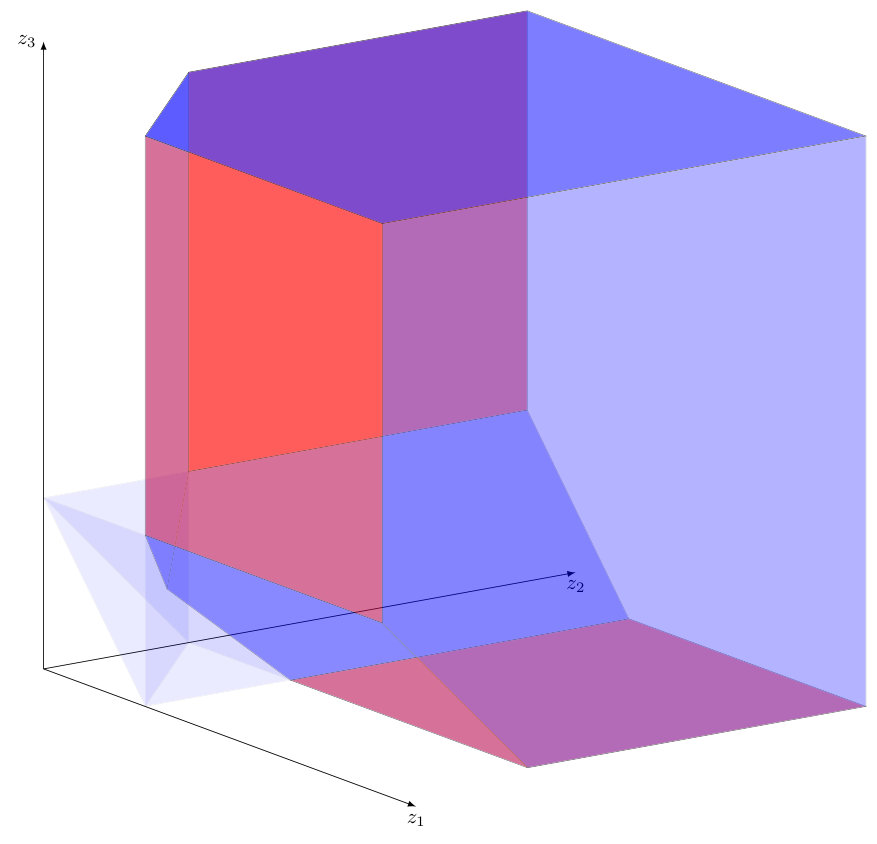 Figure 1
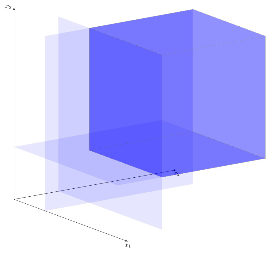 Figure 2
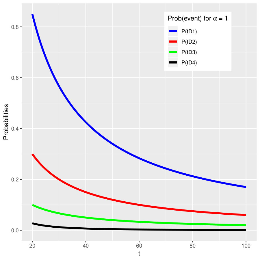 Figure 3
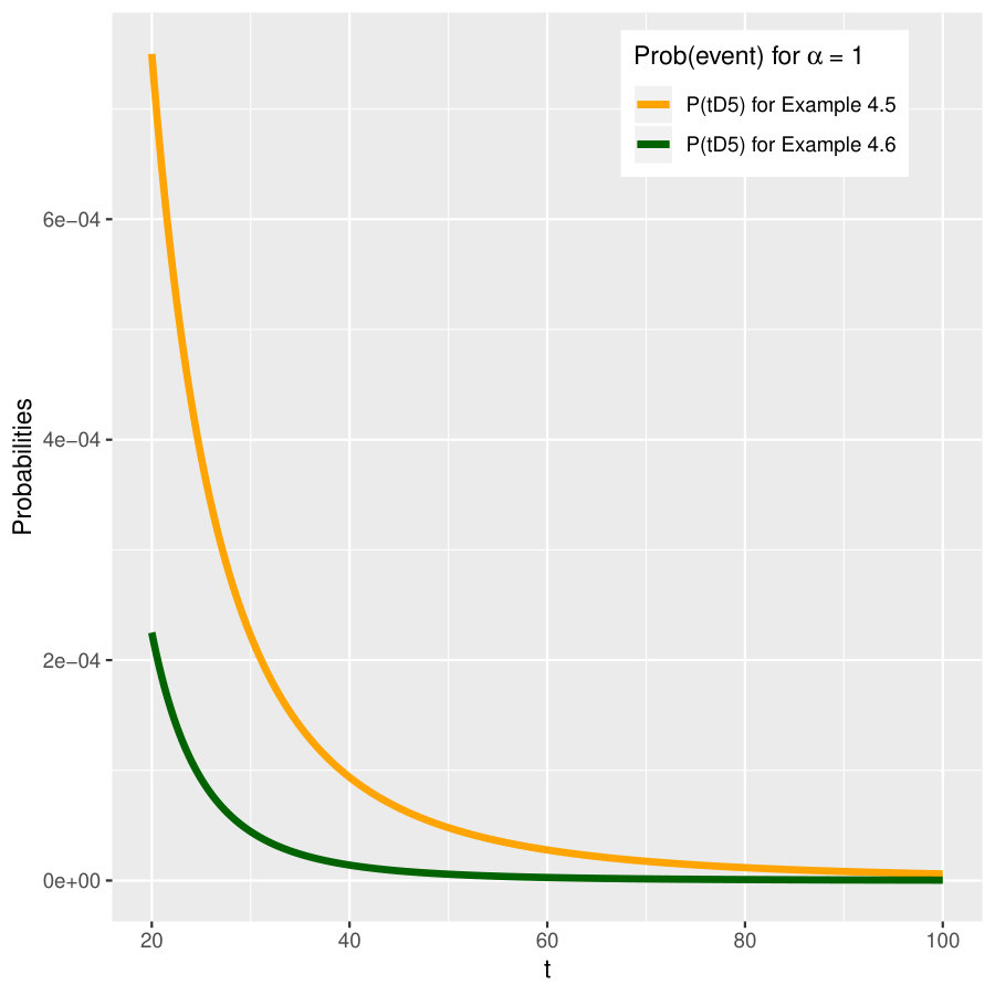 Figure 4
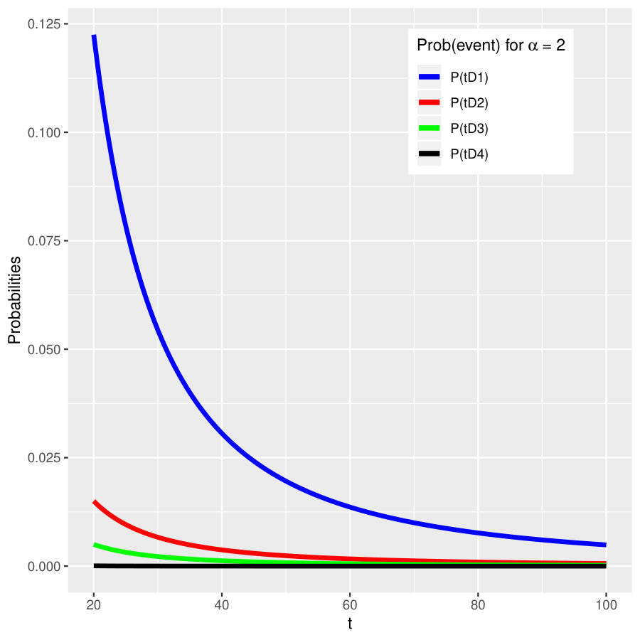 Figure 5
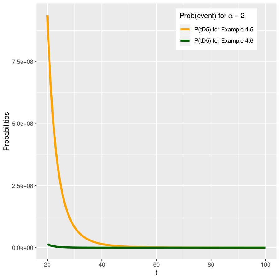 Figure 6
Peer Reviews
No public reviews on file for this paper yet. If you reviewed it on a platform where reviews are public (OpenReview, ICLR, NeurIPS, ICML), you can paste yours below so the community can read it here.
Videos
No videos yet. Explain this paper in a talk, walkthrough, or lecture? Add one.
Tail probabilities of random linear functions of regularly varying random vectors
Bikramjit Das label=e1][email protected] [ Engineering Systems and Design
Singapore University of Technology and Design
8 Somapah Road
Singapore 487372, Singapore
Singapore University of Technology and Design
Vicky Fasen-Hartmannlabel=e2][email protected] [ Institute for Stochastics
Karlsruhe Institute of Technology
Englerstrasse 2
76131 Karlsruhe, Germany
Karlsruhe Institute of Technology
Claudia Klüppelberg label=e3][email protected] [ Center for Mathematical Sciences
Technical University of Munich
Boltzmanstrasse 3
85748 Garching, Germany
Technical University of Munich
Abstract
We provide a new extension of Breiman’s Theorem on computing tail probabilities of a product of random variables to a multivariate setting. In particular, we give a complete characterization of regular variation on cones in under random linear transformations. This allows us to compute probabilities of a variety of tail events, which classical multivariate regularly varying models would report to be asymptotically negligible. We illustrate our findings with applications to risk assessment in financial systems and reinsurance markets under a bipartite network structure.
60B10,
60F10,
60G70,
90B15,
bipartite graphs,
heavy-tails,
multivariate regular variation,
networks,
keywords:
[class=AMS]
keywords:
\setattribute
journalname
\arxivmath.PR/0000000
and
and
t1B. Das was partially supported by the MOE Academic Research Fund Tier 2 grant MOE2017-T2-2-161 on “Learning from common connections in social networks”.
1 Introduction
In this article we study the probability of tail events for random linear functions of regularly varying random vectors. Throughout all random elements are defined on the same probability space . Suppose is a non-negative random vector with multivariate regularly varying tail distribution on with index , denoted as . A precise definition of this notion is given in Section 2. Furthermore, let be a random matrix independent of . For , our goal is to find for large values of and a wide variety of sets .
A classical result on the tail behavior of a product of random variables, now known as Breiman’s Theorem, states that given independent non-negative random variables and , where has a univariate regularly varying tail distribution with index and for some , the tail distribution of is also regularly varying with index . More precisely,
[TABLE]
This was stated first in Breiman (1965) for and established for all in Cline and Samorodnitsky (1991). The inherent applicability of this result to stochastic recurrence equations and portfolio tail risk computations has lead to a few generalizations in the past decades. A generalization of Breiman’s Theorem by relaxing the assumption of independence of the random variables and to asymptotic independence was provided in Maulik, Resnick and Rootzén (2002). On the other hand, a weakening of the conditions on such that (1.1) holds was given in Denisov and Zwart (2007).
A vector-valued generalization of (1.1) was obtained in Basrak, Davis and Mikosch (2002, Proposition A.1) where the -dimensional non-negative random vector for is independent of a -dimensional random matrix with for some . The result states that in such a case where . A generalization of this result with respect to the dependence and joint regular variation assumptions on was given in Fougeres and Mercadier (2012). On the other hand, Janssen and Drees (2016, Theorem 2.3) generalized Proposition A.1 in Basrak, Davis and Mikosch (2002) so that one may compute probabilities of tail sets contained in when and is of full rank (and certain other conditions). For they show that .
Consider the following example to fix ideas in this setting. Let be comprised of iid (independent and identically distributed) Pareto random variables with for , where , and let be a random matrix independent of satisfying the conditions for both Basrak, Davis and Mikosch (2002, Proposition A.1) and Janssen and Drees (2016, Theorem 2.3). Then and . Hence for sets of the form and with , we are able to compute for :
[TABLE]
for some measures and to be elaborated on later. Moreover, the expectations on the right hand side of both (1.2) and (1.3) are non-trivial and finite; hence our probability estimates are valid. Thus (1.2) allows us to compute probabilities of events described as “at least one of the components of is large”, whereas (1.3) allows us to compute probabilities of events described as “all components of are large”. Natural questions to inquire of here would be, what if we want to compute such probabilities when the matrix is not invertible, or perhaps . We may also wish to find the probability that “at least three of the components of are large” or “exactly two of the components of are large”. We can check that, although a probability computation akin to (1.2) is possible in such a case, it will often render the measure and hence, the right hand side of (1.2) to be zero. On the other hand, (1.3) will fail to answer such a question if either or the particular set of concern does not have all components to be large. To the best of our knowledge, (1.2) and (1.3) are the only results that compute probabilities of extreme sets for random linear functions of regularly varying vectors. In our work, we provide a generalization of Breiman’s Theorem which allows us to compute such probabilities for more general extreme sets. For example, in this particular setting of being iid Pareto, our results show that
[TABLE]
where the index depends on the structure of the matrix and the set , and represents an expectation over an appropriate subspace of the probability space; see Section 3.2 for the definition. Finding the correct exponent under a general set-up forms the basis of this paper.
Further related literature: A few other publications have also exhibited interesting applications and generalizations of Breiman’s Theorem, albeit in different contexts. In Jessen and Mikosch (2006), the authors provide partial converses to Breiman’s Theorem: assuming and to be non-negative independent random variables, if has a regularly varying tail distribution, they find conditions when will also have a regularly varying tail distribution. In Tillier and Wintenberger (2017) we find an extension of Breiman’s multivariate result to vectors of random length, determined for instance by a Poisson random variable. In a more general setting, Chakraborty and Hazra (2018), extend Breiman’s result for multiplicative Boolean convolution of regularly varying measures. Finally, the monograph Buraczewski, Damek and Mikosch (2016) provides many applications of Breiman’s result and its generalizations in the area of stochastic modeling with power-law tails.
Our interest in computation of probabilities of the form (1.4) is motivated by a wide range of applications in mind. Regularly varying tail distributions have been used to model power-law tail behavior in stochastic models in applications including hydrology, finance, insurance, telecommunication, social networks and many more. A regularly varying random vector like can be used to represent investment risks from multiple stocks (in finance) or losses pertaining to different insurance companies (in an insurance context). In such applications a random matrix represents randomly weighted choices of portfolios of a group of stockholders or business entities, or, randomly weighted exposures of insurance companies to losses, respectively. Thus a common quantity of interest to compute here is for tail sets representing a variety of worst case scenarios relating to multiple portfolios, or bankruptcy or loss for multiple insurers.
Our paper is organized as follows. We provide a summary of notations used in the paper in Section 1.1 to finish up the introduction. In Section 2, we discuss multivariate regular variation with -convergence in different subspaces of which provides a set up for the main result of the paper. Our main result extending Breiman’s Theorem is developed in Section 3. In Section 4, we provide applications of the model in the context of bipartite networks, where agents can be exposed to the risk of objects where are the risks of the objects. The exposures of the agents is represented by and illustrate the behavior of tail risk of the agents for possible structures of the weighted adjacency matrix . We conclude with indications to future directions of research in Section 5.
1.1 Notations
Various notations and concepts used in this paper are summarized in this section. Vector operations are always understood component-wise, e.g., for vectors and , means for all . For a constant and a set , we denote by . Further notations are tabulated below. References are provided wherever applicable.
[TABLE]
[TABLE]
2 Multivariate regular variation and convergence concepts
We use the notion of -convergence of measures to define multivariate regular variation on Euclidean spaces and subsets thereof; see Das, Mitra and Resnick (2013); Lindskog, Resnick and Roy (2014) for details. In particular, we investigate regular variation of a random vector , which is given as , where is multivariate regularly varying with index and is a random matrix independent of such that for some and some operator norm for matrices.
Our goal is to obtain a complete picture concerning linear functions which possess multivariate regular variation on a sequence of subspaces of (also called hidden regular variation), thus extending results from Basrak, Davis and Mikosch (2002); Janssen and Drees (2016). The particular choice of subsets where we seek regular variation are natural, depending on the type of extreme sets for which we seek to find probabilities; see Mitra and Resnick (2011) for examples. The necessary definitions and results formulated with respect to -convergence are discussed below.
Consider the space endowed with a metric satisfying for some
[TABLE]
Any metric defined by a norm as will always satisfy (2.1). In this paper, we use the sup-norm as our choice of metric , since the distance of a point to a specific closed set can be represented as an order statistic of the co-ordinates of ; see (3.3).
Recall that a cone is a set which is closed under scalar multiplication: if then for . A closed cone of course, is a cone which is a closed set in . Now we define multivariate regular variation using convergence of measures on a closed cone with a closed cone deleted. Moreover, we say that a subset is bounded away from if . The class of Borel measures on that assign finite measure to all Borel sets , which are bounded away from , is denoted by .
In this paper, regular variation on cones is defined using -convergence, which is slightly different from vague convergence which has been traditionally used in multivariate regular variation. Reasons for the preference of -convergence are presented in Das and Resnick (2015, Remark 1.1); see also Das, Mitra and Resnick (2013); Lindskog, Resnick and Roy (2014). In the space the notions of vague convergence and -convergence are identical.
Definition 2.1**.**
Let be closed cones containing . Let be Borel measures on and as for any bounded, continuous, real-valued function whose support is bounded away from , then we say * converges to in *, and write in .
Definition 2.2**.**
Let be closed cones containing . A random vector is regularly varying on if there exists a function for , called the scaling function, and a non-null (Borel) measure called the limit or tail measure such that
[TABLE]
in . We write or, if the scaling function is contextually irrelevant. If , we simply write or .
For , a possible choice of is given by using as . Since , the limit measure has a scaling property:
[TABLE]
2.1 Regular variation on a sequence of subspaces
We define regular variation on a specific sequence of subspaces of following Mitra and Resnick (2011). For , write . Moreover, the order statistics for any vector is defined as
[TABLE]
where denotes the -th largest component of . First we define closed sets which we think of as a union of co-ordinate hyper-planes of various dimensions in . Let and for define
[TABLE]
Here represents the union of all -dimensional co-ordinate hyperplanes in . Also define . Now define the following sequence of subcones of :
[TABLE]
Hence is the non-negative orthant with removed, is the non-negative orthant with all one-dimensional co-ordinate axes removed, is the non-negative orthant with all two-dimensional co-ordinate hyperplanes removed, and so on. Clearly, we have
[TABLE]
Note that according to our definition We also define for ,
[TABLE]
where denotes the -th -dimensional co-ordinate hyperplane in with positive and zero co-ordinates in some ordering of the hyperplanes. We note in passing that
[TABLE]
A recipe for finding regular variation in the above sequence of cones can be devised as follows. To start with, suppose with .
- (1)
If , we seek no further regular variation on cones of . 2. (2)
If , we may find an such that , yet . Hence concentrates on . So we seek regular variation in . Suppose there exists with and on such that . Then, , and for . Hence has regular variation on with parameter . 3. (3)
In the next step, if , we stop looking for regular variation; otherwise we keep seeking regular variation through sequentially.
The idea of regular variation on a sequence of cones is easier understood with an example.
Example 2.3**.**
For , suppose and are iid Pareto() random variables with such that , .
- (i)
First we observe that for all , we have with and where the limit measure on is such that for any ,
[TABLE]
This follows from Example 5.1 in Maulik and Resnick (2005) and Example 2.2 in Mitra and Resnick (2011). Hence, if
[TABLE]
we find
[TABLE] 2. (ii)
The measure as defined in (2.5) concentrates on . 3. (iii)
In general, from part (i) we conclude that for any Borel set which is bounded away from ,
[TABLE]
So, in case , we get as . However, if is of the form (2.6), or a finite union of such sets (for fixed ), from (2.7) we know that .
Remark 1**.**
Although multivariate regular variation can be defined for a very general class of cones in (see Das, Mitra and Resnick (2013); Lindskog, Resnick and Roy (2014); Mitra and Resnick (2011) for examples), for the purposes of this paper, restricting to the sub-cones defined in (2.2) and (2.3) suffices. For an example of regular variation with infinite sequence of indices on an infinite sequence of cones contained in the space , see Das, Mitra and Resnick (2013, Example 5.3).
Definition 2.4**.**
Suppose and is the generalized inverse of the distribution function of , where are the order statistics of . If , we call the canonical choice of the scaling function.
3 Breiman’s Theorem and regular variation on Euclidean subspaces
In this section we provide a complete characterization of the vector-valued generalization addressed in Basrak, Davis and Mikosch (2002, Proposition A.1) for the space and its subsequent modification for for provided in Janssen and Drees (2016, Theorem 2.3). We investigate the vector , where is a random matrix which is independent of , and is multivariate regularly varying on subspaces for . We provide asymptotic rates of convergence of tail probabilities for for Borel sets for . For the sake of convenience, first we present the two available results addressing this issue.
Throughout denotes an arbitrary vector and operator norm, only the metric is always defined by the sup-norm. Most results quoted from previous papers appeared with asymptotic properties and definitions in terms of vague convergence, we restate them here with respect to -convergence.
Theorem 3.1** **(Basrak, Davis and
Mikosch (2002, Proposition A.1)).
Let be a random vector such that with and be a random matrix independent of with for some . Then
[TABLE]
*in . In particular, we have . *
Remark 2**.**
A couple of remarks are in order here.
- (i)
For to become large, it suffices that one component of becomes large. Hence as for some constant , and provides the rate of convergence of to zero. 2. (ii)
The observation in (1.2) is an easy consequence of this theorem.
For certain sets in , it is possible that the right hand side of (3.1) turns out to be zero, rendering the result uninformative. A partial solution for guaranteeing a non-zero limit in (3.1) is provided in Janssen and Drees (2016), when and where convergence occurs in the space , which means that we focus on sets, where all components of are large, translated into the event .
The formal setting in Janssen and Drees (2016) is as follows. Define to be the distance of a point from the space in the sup-norm, given by . For a deterministic matrix we define the analog
[TABLE]
where for ,
[TABLE]
Theorem 3.2** (Janssen and Drees (2016, Theorem 2.3)).**
Let be a random vector such that and be a random matrix independent of . Assume almost surely and for some . Then
[TABLE]
*in . In particular, we have . *
Remark 3**.**
A couple of remarks are necessary to explain the result stated above.
- (i)
Note that which provides the rate of convergence of to zero as . 2. (ii)
The observation in (1.3) is an easy consequence of Theorem 3.2. 3. (iii)
Theorem 3.2 is designed for a specific situation in the context of stochastic volatility models. It is restrictive in its assumptions and may fail to capture a variety of instances where the right hand side of (3.1) is zero. In particular, for a square random matrix with almost surely non-negative entries, Theorem 3.2 requires that is almost surely invertible and, moreover, that its inverse has almost surely non-negative entries (see Janssen and Drees (2016, Lemma 2.2)). This entails that almost all realizations of are row permutations of diagonal matrices with positive diagonal entries (cf. Ding and Rhee (2014)).
3.1 Extension of Breiman’s Theorem to Euclidean subspaces
In light of the previous results, we provide a multivariate extension to Breiman’s Theorem which entails non-trivial convergence for a multitude of forms of . Let be deterministic. We define the analog sequence of subcones of as in (2.2)-(2.3) and proceed as follows. For , define to be the distance of a point from the space in the sup-norm, given by
[TABLE]
Furthermore, we define in analogy to (3.2) the function given by
[TABLE]
Note that from (3.2) if .
Although the functions are not necessarily seminorms on the induced vector space (see Horn and Johnson (2013, Section 5.1)), they admit to some useful properties as listed below. We call a row of trivial, if it is a zero vector.
Lemma 3.3**.**
For every deterministic matrix and the following hold for and :
- (a)
*. * 2. (b)
. 3. (c)
*. * 4. (d)
* if and only if all rows of are non-trivial.* 5. (e)
.
Proof.
- (a)
By definition we have
[TABLE] 2. (b)
and (c) immediately follow from the definition. 3. (d)
If has no trivial row, denoting , we have
[TABLE]
the final domination being a consequence of each row of having at least one positive entry.
On the other hand, suppose that and has a trivial row. Then for any , we have
[TABLE]
This implies
[TABLE]
which is a contradiction. Hence cannot have a trivial row. 4. (e)
The first inequality follows from (b). Moreover
[TABLE]
∎
For a deterministic matrix and , the pre-image of is given by
[TABLE]
The following lemma characterizes the mapping of the subspaces of under the linear map and is key to the results to follow.
Lemma 3.4**.**
Let be a deterministic matrix with all rows non-trivial. Then for fixed and fixed , the following are equivalent:
- (a)
.
- (b)
.
Proof.
(a)(b): Let . First suppose that . Hence by definition, from (3.4) we have that for every . Thus
[TABLE]
contradicting the premise.
Now suppose that . Let where . Then there exists a such that . Fix such a and without loss of generality assume that (otherwise we may arrange columns of accordingly). Hence . Define by converting the last components of to 1. Hence
[TABLE]
Since the components of and are ordered and component-wise , we have . Now, define
[TABLE]
Clearly as well as since . Note that means at least -elements of are larger than , whereas by definition. Hence all elements of are at most . Since , at least elements of are greater or equal to . Therefore, . Thus which is a contradiction.
(b)(a): Let . Then . Furthermore, let and let . Then by Lemma 3.3(a),
[TABLE]
implying . Hence . ∎
Example 3.5**.**
The following example illustrates the equivalence shown in Lemma 3.4. Suppose that
[TABLE]
and . Then
[TABLE]
For we find
[TABLE]
The supremum value of 3 in the first two cases is attained at for . The final equality is attained by using for , where . Hence according to Lemma 3.4 we have
[TABLE]
This means that the pre-image contains vectors , whose largest two components are positive, and the other two components can be either zero or positive.
This example can be compared to Janssen and Drees (2016, Lemma 2.2) where only is considered, which for this example is infinite by Lemma 3.3(c). The only choice for where are permutations of diagonal matrices with positive diagonal entries; see Remark 3 (iii).
3.2 Main Result
The key result extending Theorems 3.1 and 3.2, incorporating general random matrices and a wide variety of tail sets, is provided in this section. If with asymptotically independent components, implying , we may seek and find multivariate regular variation in subcones for as seen in Section 2.1. Theorem 3.6 provides the appropriate non-null limit and its rate in the presence of such regular variation for .
For and define and
[TABLE]
which creates a partition of given by
[TABLE]
We write and . This means, for fixed , we summarize all , such that yields the same , and we work on measure spaces indexed by .
Theorem 3.6**.**
Let be fixed and a random vector such that with canonical choice of as in Definition 2.4. Also let be a random matrix with almost surely no trivial rows independent of . Furthermore, assume that the following conditions are satisfied for some :
- (i)
for some we have
[TABLE] 2. (ii)
* for all .*
Then we have
[TABLE]
*in . *
Proof.
If then (3.5) is trivially satisfied because the left and right hand side are zero. Thus we assume that . Let be a Borel set which is bounded away from and satisfies . Then there exists a constant such that for all . Using Lemma 3.3(a), we have for all ,
[TABLE]
Since , and and are assumed to be independent, the univariate version of Breiman’s Theorem in combination with yields
[TABLE]
Note that is again a.s. bounded away from , since for , , and we have by Lemma 3.3(a),
[TABLE]
and, thus, . Hence abbreviating and conditioning on , by independence of and , we obtain
[TABLE]
where we used for the third equality that in combination with Pratt’s lemma (Pratt, 1960), since for we have for the integrand
[TABLE]
We need to show that . Define . By the homogeneity of and (3.6) we have
[TABLE]
To finish the proof it remains to show that
Case 1: Suppose . Let . We know from Lemma 3.4 that . By definition, . We claim that
[TABLE]
If not, then we have . Therefore by Lemma 3.4, . But this is a contradiction to the definition of since .
So let . Then by (2.4), we have for some . Let . Clearly,
[TABLE]
Hence for every we have that some component of is positive if and only if the corresponding component of is positive, since has only non-negative entries. Thus , i.e., . Hence, we get that
[TABLE]
Since due to assumption (ii), has positive mass on each of the hyperplanes , this results in
[TABLE]
and
[TABLE]
which proves the claim for .
Case 2: Suppose . Let . Take , then all components of and are positive. Thus has no trivial row and we get that for every also has only positive components, i.e., . This results in and . ∎
Remark 4**.**
The condition that for all could be relaxed to for at least one , but showing that the limit measure is non-zero turns out to be a cumbersome exercise and needs to be done with proper care. In many examples, the measures turn out to be exchangeable with respect to their co-ordinates and the assumption being true for all is not uncommon. One such example is given in Example 2.3 where are iid Pareto for and we have for all .
Theorem 3.6 provides regular variation limit measures for sets in restricted to , whenever the two conditions are satisfied and, as a consequence, we have the following limit probabilities.
Theorem 3.7**.**
*Let be a random vector such that for all , we have with canonical choice of as in Definition 2.4. Moreover, for all we assume as . Let be a random matrix with almost surely no trivial rows independent of . Furthermore, let for be a Borel set bounded away from with for all .
Suppose further that*
- (i)
* for some ,* 2. (ii)
* for all .*
*Then the following results hold. *
- (a)
We have
[TABLE] 2. (b)
Define
[TABLE]
Then we have
[TABLE]
in . Hence, .
Proof.
- (a)
Since forms a partition of , . Hence using (3.5) and observing that
[TABLE]
we have
[TABLE] 2. (b)
Now, since forms a partition of , there exists a with and hence, is well-defined. Note that using (3.7), we have for any Borel set bounded away from with for , the following asymptotic behavior:
[TABLE]
since for all we have , and hence
[TABLE]
Hence .
∎
Remark 5**.**
When we assume for all , with as for all , it results in restricting the supports for the measures to ; a specific case is discussed in Example 2.3.
Remark 6**.**
If has asymptotically independent components, and each component has distribution tail as for some , then we get a generalization of Theorem 3.2 of Kley, Klüppelberg and Reinert (2016). We investigate such structures further in the next section.
The following example illustrates the image and pre-image of sets under the map as well as the regions, where the limit measure is positive in a 3-dimensional setting. We emphasize that for this example our theory is not really necessary, the calculations can be done by hand, but it helps in clarifying the ideas and the notation needed for more complex examples to follow.
Example 3.8**.**
Let have iid Pareto() marginal distributions with for some as in Example 2.3. Then for where and are the canonical choices and
[TABLE]
for . Consider the matrix
[TABLE]
Then, under the map , the region has pre-image given by
[TABLE]
It is easy to check that , as defined in (3.8). Hence, with we obtain
[TABLE]
Figure 1 gives a plot of the region and the transformed region colored in blue. The red region on the right plot shows the support of the measure .
Remark 7**.**
In Theorem 3.7, we ascertain the asymptotic behavior of for certain sets . Specifically, from Theorem 3.7 (b) we have
[TABLE]
where is defined in (3.8). If , we only get
[TABLE]
However, under certain assumptions on and we can say more about the precise rates, illustrated in the following results.
Proposition 3.9**.**
*Let the assumptions and notations of Theorem 3.7 hold. Define *
[TABLE]
Suppose for all and that . Then
[TABLE]
Proof.
Since by assumption, for all and , we have , we obtain
[TABLE]
Therefore due to the definition of ,
[TABLE]
using Theorem 3.6.∎
The additional assumption made in Proposition 3.9 is often satisfied by random matrix structures. One such example is a random matrix with only one positive entry in each row. Such matrices are for instance proposed in the examples of Section 4.1. Moreover, if and we follow the assumptions of (Janssen and Drees, 2016, Theorem 2.3), we also obtain such matrices; cf. Remark 3(iii). The following proposition formalizes the result in this case.
Proposition 3.10**.**
Let the assumptions and notations of Theorem 3.7 hold. Moreover, let be such that for some , where each is of the form:
[TABLE]
and for all . Let be defined as in (3.9). If the random matrix has a discrete distribution and has exactly one positive entry in each row, then (3.10) holds.
Proof.
If we show that for all and , we have , then applying Proposition 3.9 we get the result. Fix . By definition, we have . Suppose there exists with
[TABLE]
Then there exists and with .
Since , exactly components of are positive. Without loss of generality let Now for any with , we have and by the structure of , we have Hence
[TABLE]
Now from assumption (ii) of Theorem 3.7 and the homogeneity of the measure , we have
[TABLE]
since has a discrete distribution and . Hence , which is a contradiction. Thus
[TABLE]
Now suppose that . Then there exist and with . Since , exactly columns of have at least one positive entry. W.l.o.g. assume these are the first columns of . Then for
[TABLE]
we have
[TABLE]
since columns of have all entries zero and hence the last entries of or do not count towards the computation of . Hence , which is a contradiction to (3.12). This gives the statement. ∎
4 Bipartite networks
Risk-sharing in complex systems is often modeled using a graphical network model, one such example being the bipartite network structure for modeling losses in insurance markets or financial investment risk as proposed in Kley, Klüppelberg and Reinert (2016, 2018). In these papers, only first order asymptotics of risk measures based on the agents’ and market’s tail risks are derived. In the same spirit, but going beyond first order approximations, we consider a vertex set of agents and a vertex set of objects (insurance claims or investment risks) .
Each agent chooses a number of objects to connect with. Figure 2 provides an example of such a network. This choice can be random according to some probability distribution. A basic model assumes and connect with probability
[TABLE]
Let denote the risk attributed to the -th object and forms the risk vector. Assume that the graph creation process is independent of . The proportion of loss of object affecting agent is denoted by
[TABLE]
where denotes the effect of the -th object on the -th agent. Now define the weighted adjacency matrix by
[TABLE]
The total exposure of the agents given by , where can be represented as
[TABLE]
Our goal is to find the probability of tail risks of some or all agents in terms of .
In Kley, Klüppelberg and Reinert (2016, 2018), proportional weights are used to distribute the insurance loss of object affecting agent or to diversify the investment risk of an agent. The weights complicate calculations and only affect the values of the limit measures, resulting in different constants, whereas the rate of convergence remains the same. As they rather blur the mathematical insight, we work in Section 4.1 with unweighted adjacency matrices. However, they can be incorporated in the calculations by appropriate multiplications using the independence of and . We consider a weighted adjacency matrix in Section 4.2, when we investigate dependent objects in contrast to independent ones; see Examples 4.4 and 4.5 below. Throughout we formulate our examples and results in terms of investment risk.
4.1 Independent objects
For illustration we start with an example, which shows how regular variation of for independent Pareto-tailed components of and random adjacency matrices transforms into regular variation of . The choice of specifies the tail risk, and in this example we calculate the asymptotic tail risk explicitly for two different kinds of sets leading to two different asymptotic rates.
Example 4.1**.**
Suppose there are two products and in the market with associated risks and respectively, which are independent and for as with constants for . Assume there are three investors, each of whom may either invest in one unit of or one unit of or one unit of both (we assume that they always invest). Hence there are possible market investments which may be represented by the matrix so that the joint risk of the investors is given by Now the 27 possibilities for the matrix are given by
[TABLE]
[TABLE]
[TABLE]
[TABLE]
[TABLE]
and let for such that , and .
Suppose we want to assess the risk of all investors being above a high threshold . Moreover, we also want to find the probability that when all risks of the investors are above , the risk of the first investor is larger than that of the second which is larger than the one of the third, i.e., . Hence given and
[TABLE]
we want to compute for First note that and where and for
[TABLE]
In order to compute the necessary probabilities, we first need to compute as defined in Theorem 3.7 based on for and . We can check that for ,
[TABLE]
Hence for , we get for On the other hand for , we observe that
[TABLE]
Therefore for , we get and
Clearly from our assumptions,
[TABLE]
where
[TABLE]
Note that both . Applying Theorem 3.7(b) results in and we have
[TABLE]
First consider the set as defined in (4.2). Since
[TABLE]
we have
[TABLE]
The same result can be obtained from Proposition 3.9, since (4.4) indicates Now consider the set as in (4.3). Note that in this case,
[TABLE]
Hence using notation from Proposition 3.9, we have . Furthermore, for we have . Therefore the assumptions of Proposition 3.9 are satisfied and we obtain
[TABLE]
Examples for different choices of risk sets are aplenty considering the numerous risk situations for a group of agents. In what follows, we address tail risks for extreme events where the portfolio risk of all agents are above a high threshold in a more systematic way. Such events are represented by sets of the form . In case we want to study the problem for a specific set of agents, we need only to consider a reduced set of rows of the adjacency matrix .
We suppose that each agent is able to take investment decisions according to a probability distribution, where the agents’ choices are independent of each other. Hence, we may assume for each agent that there exist subsets of investments such that
[TABLE]
for and . We may also consider for as in (4.1).
Our examples also show exactly how our results extend those of Theorem 3.2 of Janssen and Drees Janssen and Drees (2016) in multiple directions. Firstly, we allow for a non-square matrix with , whereas the result in Janssen and Drees (2016) was restricted to . For computational ease we restrict to the case where the components of are independent. Although this results in as required in Janssen and Drees (2016), we obtain to be multivariate regularly varying with different indices in different spaces; whereas in the aforementioned paper, the indices of regular variation of and on remain identical.
Our first result provides tail probabilities for the agents’ risk exposures for a model, where each agent invests in exactly one investment possibility and the investment possibilities are independent of each other. Moreover, agents take their investment decisions independently.
To invest into one investment possibility is a risk averse investment strategy for small . According to Remark 13.3(b) of Rüschendorf Rüschendorf (2013), for portfolio diversification does not reduce the danger of extreme losses, but typically increases extreme risks.
Proposition 4.2**.**
Let be independent random variables such that for as with constants for . Let for be a random adjacency matrix, where for all independently,
[TABLE]
- (a)
For we have with
[TABLE]
where for and . 2. (b)
We have and for and we have as ,
[TABLE]
where
[TABLE] 3. (c)
For we have with where and
[TABLE]
such that for as ,
[TABLE]
Proof.
First note that using similar arguments as in Lemma 2.3, we have for any that with canonical choices and
[TABLE]
Moreover, for we have
[TABLE]
and
[TABLE]
The structure of guarantees that \mathbf{E}_{i}^{(q)}\big{[}\tau_{q,d}^{(k,i)}(\boldsymbol{A})^{i\alpha}\big{]}=1, satisfying condition (i) of Theorems 3.6 and 3.7. Also, referring to Remark 4 and (4.1), we have for all , satisfying condition (ii) in Theorems 3.6 and 3.7. Now we show the various parts of the result.
- (a)
Let . Then and hence, the conclusion follows from Theorem 3.7. 2. (b)
Since each row of has exactly one entry 1 and all others zero, we have for ,
[TABLE]
because if and only if there are not more than columns of with positive entries.
Clearly and we have .
Now for and define
[TABLE]
Hence for ,
[TABLE]
Now an application of Theorem 3.6 yields
[TABLE]
which is the result in (b). 3. (c)
Using notation from Theorem 3.7, we have . Also note that for ,
[TABLE]
Therefore using Theorem 3.7(b) we have and as ,
[TABLE]
which shows (c).
∎
Proposition 4.2 shows that for sets for , is of the order . But for sets of the form which belong to , we observe a tail probability of the order . However, if we restrict to as in part (b), we may observe tail probabilities of the order for all .
In the next example we show that tail probabilities of other orders can also be observed for risk sets of the form . Here we fix and consider the same investment scenario as in Proposition 4.2; i.e., each agent invests in exactly one investment possibility and agents take their investment decisions independently. As before each row is a unit vector, but the distribution of changes. Given , the single 1 in each row is chosen uniformly on a subset of size , the subset changing across each row.
From a mathematical point of view, we obtain multivariate regular variation with different indices on depending on the choice of . Such a model leads to explicit expressions for the asymptotic tail probabilities for .
Proposition 4.3**.**
Let be independent random variables such that for as with constants for . Let , and be a random adjacency matrix, where for all independently
[TABLE]
where is defined as
[TABLE]
Also define for ,
[TABLE]
Then the following assertions hold:
- (a)
For we have with
[TABLE]
and for we have with
[TABLE]
*where , is defined as in (4.1), and with as in (4.6). * 2. (b)
For , and we have as ,
[TABLE] 3. (c)
For , part (a) applies with
[TABLE]
with as in (4.6), and we have as ,
[TABLE]
Proof.
For ,
[TABLE]
such that and . The proposition can then be proved in a similar manner as Proposition 4.2, and is omitted here. ∎
4.2 Dependent objects
In this section we contrast independent objects as we have considered previously with a specific dependence structure of the components of . Moreover, we also investigate the influence of weights in a numerical example. Let be the investment portfolios of five agents, each of whom connects to a subset of three objects whose risks are given by . We estimate the tail risks for :
[TABLE]
We use a weighted adjacency matrix, which is now, however, deterministic and in both examples given by
[TABLE]
with weights . Also for the convenience of computing the limit measures of the sets we assume and .
Moreover, we assume that has a probability distribution given by
[TABLE]
for , where . For the components of are independent Pareto (cf. Example 4.4) and for they are dependent (cf. Example 4.5). Such dependence in terms of copulas has been discussed in Rodríguez-Lallena and Úbeda Flores (2004).
This setting implies that in the two examples below, the underlying distribution of has either independent marginals or at least it has a tractable form; the adjacency matrix is relatively simple, in order to provide an interpretable illustration.
Example 4.4**.**
Suppose are independent random variables such that with constants for .
We calculate all relevant quantities. First, the tails of the order statistics are given for ,
[TABLE]
We have with canonical given by
[TABLE]
and limit measures
[TABLE]
Note that for . We can check from the form of that
[TABLE]
Hence using Theorem 3.7, along with (4.10) and (LABEL:eq:mui), we have as ,
[TABLE]
Similarly, we can show that as ,
[TABLE]
The forms for and become more complicated if we do not assume . Furthermore, if all weights are equal to one, the above formulas hold true.
As an illustration, we fix . Moreover, let , , and . The five probabilities obtained above are plotted for the case in Figure 3 for . We also compare the probability for the event in this example and in Example 4.5; see the right two panels of Figure 3.
Example 4.5**.**
Suppose are dependent with joint distribution (4.9) for . Otherwise assume the setting as in Example 4.4 We calculate again all relevant quantities. First, the tails of the order statistics are given for ,
[TABLE]
Notice that the only difference from (4.10) is in the term . Hence, for we have with canonical choice for as in (4.11) and as in (LABEL:eq:mui). On the other hand, we have with
[TABLE]
and
[TABLE]
As in Example 4.4, we have Using Theorem 3.7, along with (4.10) and (LABEL:eq:mui), we have the same limits for for . The only difference occurs for , where we have for ,
[TABLE]
Again we fix and let , , and , as in Example 4.4. The probabilities for events asymptotically remain the same as in Example 4.4 (matching the plots in the left two panels of Figure 3 for the case ). In the right panels Figure 3 we plot the values for when ; clearly these values differ in the two examples.
5 Conclusion
This work is motivated by the need to find probabilities of a variety of extreme events under a linear transformation of regularly varying random vectors. By an extension of Breiman’s Theorem we have shown that probabilities of many such events can be calculated, if we have information on the regular variation property of the underlying random vector on specific subcones of the positive quadrant. Most of the subsets of such cones have linear boundaries and hence form a polytope, whose pre-image under linear transformation also turns out to be a polytope in . Computing the limit measures in such cases means finding the appropriate boundaries of the polytope which can become quite complicated. For moderate dimensions of the matrix , numerical solutions can be obtained even when the distributional forms of and are more complicated.
We envisage wide application of such results in areas of risk management. There are clear implications for computing conditional value at risk, as well as a variety of conditional risk measures. We also believe that an alternative characterization of the rate of decay of tail probabilities can be provided via connectivity of the row components (in the bipartite network model, the agents); this work is under current investigation.
The reference list from the paper itself. Each links out to its DOI / PubMed record.
- 1Basrak, Davis and Mikosch (2002) {barticle} [author] \bauthor \bsnm Basrak, \bfnm B. \binits B., \bauthor \bsnm Davis, \bfnm R. A. \binits R. A. and \bauthor \bsnm Mikosch, \bfnm T. \binits T. ( \byear 2002). \btitle Regular variation of GARCH processes. \bjournal Stoch. Proc. and their Appl. \bvolume 99 \bpages 95–115. \endbibitem
- 2Bingham, Goldie and Teugels (1989) {bbook} [author] \bauthor \bsnm Bingham, \bfnm N. H. \binits N. H., \bauthor \bsnm Goldie, \bfnm C. M. \binits C. M. and \bauthor \bsnm Teugels, \bfnm J. L. \binits J. L. ( \byear 1989). \btitle Regular Variation. \bseries Encyclopedia of Mathematics and its Applications \bvolume 27. \bpublisher Cambridge University Press, \baddress Cambridge. \endbibitem
- 3Breiman (1965) {barticle} [author] \bauthor \bsnm Breiman, \bfnm L. \binits L. ( \byear 1965). \btitle On some limit theorems similar to the arc-sin law. \bjournal Theory Probab. Appl. \bvolume 10 \bpages 323–331. \endbibitem
- 4Buraczewski, Damek and Mikosch (2016) {bbook} [author] \bauthor \bsnm Buraczewski, \bfnm D. \binits D., \bauthor \bsnm Damek, \bfnm E. \binits E. and \bauthor \bsnm Mikosch, \bfnm T. \binits T. ( \byear 2016). \btitle Stochastic Models with Power-law Tails. \bseries Springer Series in Operations Research and Financial Engineering. \bpublisher Springer. \endbibitem
- 5Chakraborty and Hazra (2018) {barticle} [author] \bauthor \bsnm Chakraborty, \bfnm S. \binits S. and \bauthor \bsnm Hazra, \bfnm R. S \binits R. S. ( \byear 2018). \btitle Boolean convolutions and regular variation. \bjournal ALEA Lat. Am. J. Probab. Math. Stat. \bvolume 15 \bpages 961–991. \endbibitem
- 6Cline and Samorodnitsky (1991) {barticle} [author] \bauthor \bsnm Cline, \bfnm D. B. H. \binits D. B. H. and \bauthor \bsnm Samorodnitsky, \bfnm G. \binits G. ( \byear 1991). \btitle Subexponentiality of the product of independent random variables. \bjournal Stoch. Proc. and their Appl. \bvolume 49 \bpages 75-98. \endbibitem
- 7Das, Mitra and Resnick (2013) {barticle} [author] \bauthor \bsnm Das, \bfnm B. \binits B., \bauthor \bsnm Mitra, \bfnm A. \binits A. and \bauthor \bsnm Resnick, \bfnm S. I. \binits S. I. ( \byear 2013). \btitle Living on the multidimensional edge: seeking hidden risks using regular variation. \bjournal Adv. in Appl. Probab. \bvolume 45 \bpages 139–163. \endbibitem
- 8Das and Resnick (2015) {barticle} [author] \bauthor \bsnm Das, \bfnm B. \binits B. and \bauthor \bsnm Resnick, \bfnm S. I. \binits S. I. ( \byear 2015). \btitle Models with hidden regular variation: Generation and detection. \bjournal Stochastic Systems \bvolume 5 \bpages 195-238. \endbibitem