On the two-body decay processes of the predicted three-body $K^*(4307)$ resonance
Xiu-Lei Ren, Brenda B. Malabarba, K. P. Khemchandani, A. Martinez, Torres

TL;DR
This paper calculates the decay processes of a theoretically predicted exotic $K^*(4307)$ resonance with hidden charm, providing decay widths that can guide experimental searches and help understand its internal structure.
Contribution
It presents the first detailed calculation of the decay channels of the $K^*(4307)$ resonance, linking its decay widths to its exotic nature and internal structure.
Findings
Decay widths for $J/\psi K^*$, $\bar{D}D_s$, $\bar{D}D_s^*$, and $\bar{D}^* D_s^*$ channels.
Decay mechanisms involve triangular loops related to the resonance's internal structure.
Results support the $K^*(4307)$ as an exotic meson with hidden charm, not a simple quark-antiquark state.
Abstract
In a recent theoretical work, Phys. Lett. B785, 112 (2018), we proposed that a resonance with hidden charm content arises from the dynamics, where the system is treated as a or . With the motivation of determining its further properties, which can be observed in experiments, we now present a calculation of the decay processes of this , namely , to two-body channels. Particularly, we consider the decay channels , , and . The mechanisms of the decay to these channels involve triangular loops and are a consequence of the internal structure of the state. Thus, the values found for the decay widths of the proposed are related to its nature and should be valuable for carrying on an experimental study of the . A state with such a mass (in…
Click any figure to enlarge with its caption.
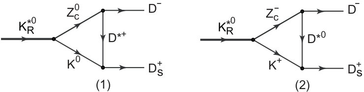 Figure 1
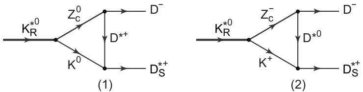 Figure 2
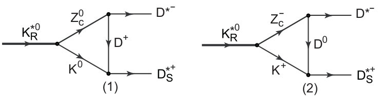 Figure 3
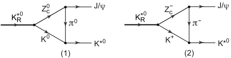 Figure 4
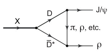 Figure 5
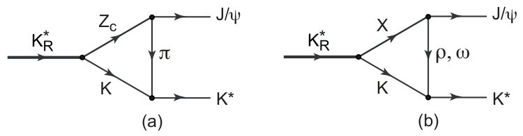 Figure 6
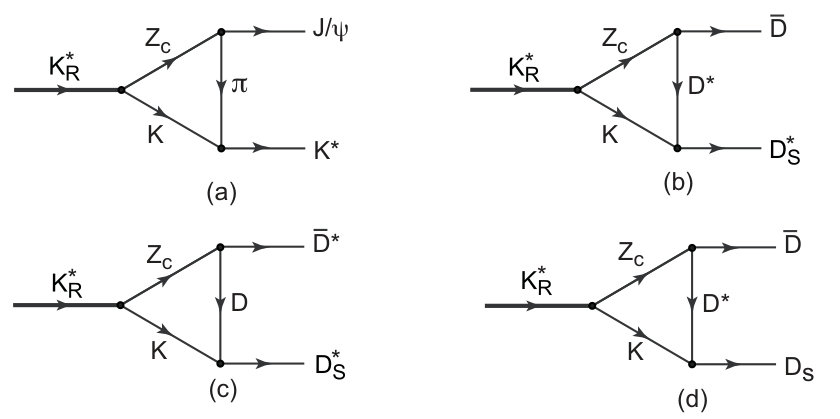 Figure 7
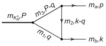 Figure 8
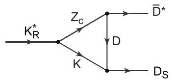 Figure 9
Peer Reviews
No public reviews on file for this paper yet. If you reviewed it on a platform where reviews are public (OpenReview, ICLR, NeurIPS, ICML), you can paste yours below so the community can read it here.
Videos
No videos yet. Explain this paper in a talk, walkthrough, or lecture? Add one.
††institutetext: Ruhr-Universität Bochum, Fakultät für Physik und Astronomie, Institut für Theoretische Physik II, D-44780 Bochum, Germany.††institutetext: Instituto de Física, Universidade de São Paulo, C.P. 66318, 05389-970 São Paulo, São Paulo, Brazil.††institutetext: Universidade Federal de São Paulo, C.P. 01302-907, São Paulo, Brazil.††institutetext: Instituto de Física, Universidade de São Paulo, C.P. 66318, 05389-970 São Paulo, São Paulo, Brazil.
On the two-body decay processes of the predicted three-body resonance
Xiu-Lei Ren
Brenda B. Malabarba
K. P. Khemchandani
A. Martínez Torres
Abstract
In a recent theoretical work, Phys. Lett. B785, 112 (2018), we proposed that a resonance with hidden charm content arises from the dynamics, where the system is treated as a or . With the motivation of determining its further properties, which can be observed in experiments, we now present a calculation of the decay processes of this , namely , to two-body channels. Particularly, we consider the decay channels , , and . The mechanisms of the decay to these channels involve triangular loops and are a consequence of the internal structure of the state. Thus, the values found for the decay widths of the proposed are related to its nature and should be valuable for carrying on an experimental study of the . A state with such a mass (in the charmonium region) and quantum numbers is a clear manifestation of an exotic meson, since, having hidden charm (i.e., a pair), its mass and quantum numbers can not be explained within a quark-antiquark description.
1 Introduction
The existence of exotic mesons and baryons, whose masses, widths and/or quantum numbers can not be explained within the constituent quark model of Gell-Mann and Zweig, is one of the peculiar characteristics of Quantum Chromodynamics which has been, and still is being, intensively explored in experiments and in theory. Typical examples are: the scalar nonet in the meson sector, which includes the , , , states Jaffe:1976ig ; Weinstein:1982gc ; vanBeveren:1986ea ; Tornqvist:1995kr ; Oller:1997ng ; Oller:1998hw , and the in the baryon sector Dalitz:1959dn ; Dalitz:1960du ; Kaiser:1995eg ; Oset:1997it ; Meissner:1999vr . With the increase of the accessible energy range by the experimental facilities, claims for the observation of such states, especially in the heavy quark sector, with a hidden charm content, started appearing in the last decade, as the so called , and families (see, e.g., Refs. Klempt:2007cp ; Brambilla:2010cs ; Hosaka:2016pey ; Oset:2016lyh ; Lebed:2016hpi ; Chen:2016qju ; Olsen:2017bmm ; Guo:2017jvc ; Liu:2019zoy for reviews on the topic). In case of the family, consisting of charged particles with masses in the charmonium mass range, 3.94.2 GeV, at least two quarks and two antiquarks are necessarily required, with a pair being responsible for their heavier masses. The isoscalar partners, belonging to the and families, are also categorized as exotic, not due to the fact that to obtain their quantum numbers we need to invoke a different structure to that of , but because their masses and widths cannot be explained within the traditional constituent quark model Chen:2016qju ; Guo:2017jvc .
All these heavy exotic mesons found experimentally in the recent years share a common feature: they are mesons with no strangeness. A glance at the Particle Data Book (PDB) Tanabashi:2018oca shows a low activity in the strange pseudoscalar and vector meson sectors since the last 30 years: in the pseudoscalar sector, the last Kaon state reported corresponds to . Its existence was claimed in 1983 from a partial wave analyses of the system produced in the reaction Armstrong:1982tw , and, recently, the LHCb collaboration took it into account in the amplitude analysis of the decay Aaij:2016iza . Similarly, in the vector sector, the latest state listed in Ref. Tanabashi:2018oca is the , whose existence dates to experiments and partial wave analysis performed during 1978-1988 Estabrooks:1977xe ; Etkin:1980me ; Aston:1986jb ; Aston:1987ir . As in the case of also, the LHCb collaboration has recently considered its existence in the analysis of the amplitude for the decay process Aaij:2016iza . And, overall, the final excited state in the meson sector, with nonzero strangeness quantum number, reported in the PDB corresponds to , whose quantum numbers are unknown, and which was observed in several pions reactions during the years 1986-1993 Aaij:2016iza .
In view of such a panorama, it is worth to explore whether or not there could be another family member to be added to the already known , , families whose members will also have masses in the charmonium mass range, i.e., GeV, but nonzero strangeness. Such states are manifestly exotic, since within a quark description, we will need at least a pair as well as a quark and a light antiquark (, ) to account for their masses and quantum numbers. Surprisingly, although being currently accessible, the existence of such states has not been yet explored experimentally. But formation of such states has been claimed theoretically very recently using different models: in Ref. Ma:2018vhp , the system was studied by solving the Schrödinger equation and considering a pion exchange potential model to describe the interactions between the pairs forming the three-body system. As a result, a bound state with mass MeV was obtained. Considering -parity arguments, the authors of Ref. Ma:2018vhp claim also the existence of a bound state with basically the same mass. In Ref. Ren:2018pcd , the system was studied by solving the Faddeev equations under the fixed center approximation Kamalov:2000iy ; Xie:2010ig ; Roca:2010tf ; MartinezTorres:2010ax ; Bayar:2011qj ; Bayar:2015oea ; Debastiani:2017vhv ; Ren:2018qhr . In this case, the interaction between the particles in the two-body subsystems were obtained by solving the Bethe-Salpeter equation in coupled channels with a kernel determined from an effective field theory implementing symmetries like the chiral symmetry Gasser:1983yg ; Gasser:1984gg or the heavy quark spin symmetry Voloshin:1978hc ; Isgur:1989vq ; Burdman:1992gh . Under such an approach, the states , and are generated from the coupled channel dynamics and are mainly bound states in isospin 0, states in isospin 0 and 1, respectively Gamermann:2006nm ; Guo:2006fu ; Nieves:2012tt ; Aceti:2014uea . As a consequence of the dynamics involved, a theoretical evidence for an state with a mass of MeV was obtained when the system clusters as or .
Theoretically, the attraction in the and subsystems, which leads to the generation of the , and states, constitutes a compelling argument in favor of the existence of such exotic state with a mass around 4.3 GeV and hidden charm. Experimentally, observation of such state should be possible in the current facilities and it would constitute an exciting novelty in the Kaonic spectroscopy and in that of the exotic mesons.
In the present work, we continue with the investigation of the properties of the state predicted in Ref. Ren:2018pcd and calculate the decay widths to several open two-body channels. Particularly, we consider the channels , , and , which are the most relevant ones, based on the nature of . This information should be reliable for experimental searches of the state proposed in Ref. Ren:2018pcd , since the decay mechanism of the state is linked to the internal structure of the decaying particle.
2 Theoretical Framework
The coupled channel calculation of Ref. Ren:2018pcd shows that the rescattering of a Kaon with the and , which cluster to form in isospin 0 and in isospin 1, generates a state with a mass around 4307 MeV, which is below the threshold, thus, it is a bound state. When considering the width of , which is around 28 MeV, a width close to 18 MeV is found for the state. A state with such an internal structure can naturally decay to three-body channels, like , since the state itself is obtained as a consequence of the three-body dynamics involved in the system. However, it can also decay to two-body channels. In this latter case, due to the nature found for in Ref. Ren:2018pcd , such a decay mechanism can proceed through triangular loops (see Fig. 1) and we can have as main decay channels , , , and (see Fig. 2). In order to avoid confusion between and and to simplify the notation, we shall, henceforth, denote the former as and the latter as .
From the results of Ref. Ren:2018pcd , the coupling of to is around 4 times bigger than that to , thus, when calculating the decay width of (which is proportional to the squared coupling of to or ), the contribution arising from the diagram shown in Fig. 1(b) is negligible when compared to the one coming from the diagram in Fig. 1(a). On top of that, for the decay process , the vertex shown in Fig. 1(b) involves yet another triangular loop Aceti:2012cb (see Fig. 3) and such a vertex produces a contribution much smaller than that of the vertices , , , since couples directly to , (where c.c means complex conjugate) Aceti:2014uea , at the tree level.
It is also interesting to notice that, with the internal structure found in Ref. Ren:2018pcd for the predicted , the decay process could also be contemplated, but it would involve a three pseudoscalar vertex (see Fig. 4), resulting in a null amplitude.
2.1 Determination of the vertices
Let us then start evaluating the contribution arising from the diagrams shown in Fig. 2. Considering the decay of a neutral into a and a , we have two diagrams contributing to each of the processes shown in Fig. 2: in one of the diagrams, the primary vertex is while in the other it is the vertex . We illustrate these two contributions in Fig. 5 for the decay process .
To evaluate these diagrams, we need several vertices involving vector and pseudoscalar mesons. The contribution for the vertices in Fig. 5 can be written in terms of the polarization vectors and associated with the vector mesons and , respectively, and the coupling of to the channel as
[TABLE]
where the four momenta and masses assigned to the particles are as shown in Fig. 6.
The couplings and in Eq. (1) can be obtained from the isospin 1/2 scattering matrix, , determined in Ref. Ren:2018pcd . To do this, we consider, a Breit-Wigner expression for this -matrix in an energy region around the mass of the state, i.e.,
[TABLE]
and we can get , i.e., the coupling of to the isospin 1/2 state , from the residue of at the pole position in the complex energy plane. Alternatively, since the decay width of is proportional to , we can estimate such a value directly from Eq. (2), by considering the limit Nagahiro:2008um
[TABLE]
Once we have the value of , the couplings and can be related to by using the fact that
[TABLE]
where we use the phase convention . In this way, from Eq. (4),
[TABLE]
Using isospin average masses for the particles belonging to the same isospin multiplet and Eq. (5), we can write Eq. (1) as
[TABLE]
with
[TABLE]
Next, we need the vertices , , for different charge combinations. As shown in Ref. Aceti:2014uea , a state with mass around 3872 MeV and 30 MeV of width is generated from the dynamics present in the (c.c. means complex conjugate) and coupled channel system in isospin 1 and positive -parity. This state can be related to Aceti:2014uea .
A comment regarding this latter state is here in order: the nature of is still under debate. Experimental investigations seem to report two states with around 3900 MeV, Ablikim:2013mio ; Liu:2013dau ; Xiao:2013iha and Ablikim:2013xfr ; Ablikim:2015swa . It is still not clear if these states are two different ones or are the same. The lattice investigations Prelovsek:2013xba ; Prelovsek:2014swa ; Chen:2014afa , on the other hand, do not seem to find an evidence for the existence of a molecular state around 3900 MeV. However, the analysis made in Ref. Albaladejo:2016jsg shows that the lattice data is compatible with the existence of the resonance. Further, the latest experimental investigations continue to find signals of a state with mass near 3900 MeV in different processes, such as -decays Abazov:2018cyu , invariant mass spectra Yuan:2018inv , etc. In spite of the debate, both experimental and theoretical investigations indicate that the interaction in isospin 1, spin-parity is attractive in nature and produces a peak in the cross sections of the relevant processes. In our study, the we refer to is the state arising from the and coupled channel dynamics found in Ref. Aceti:2014uea .
Following the approach of Ref. Aceti:2014uea , we can write
[TABLE]
where we have defined
[TABLE]
The subscript 1 in the above equation indicates the total isospin of the system. The and coefficients in Eq. (10), which relate the state to the and states in the charge basis, are given by
[TABLE]
where we have used the isospin phase convention and . In case of pions, we follow the isospin phase convention . In this way, for the processes and .
The couplings in Eq. (10) can be obtained from the residue of the isospin 1 two-body scattering matrix determined in Ref. Aceti:2014uea in the complex energy plane. We have calculated them and obtain
[TABLE]
Other vertices needed to evaluate the contribution of the diagrams shown in Fig. 2 are , and . To determine these contributions, we use the effective Lagrangian Bando:1987br ; Oset:2009vf involving two pseudoscalars and a vector meson
[TABLE]
with and being matrices containing the corresponding vectors and pseudoscalar fields,
[TABLE]
respectively. The coupling in Eq. (18) is given by , with MeV being an average mass for the vector mesons , and and MeV being the pion decay constant. While this value of the coupling produces a theoretical width of the meson, which comes basically from the decay processes , , compatible with the experimental result, it underestimates the width of the meson, obtained from the processes , . In this latter case, as shown in Ref. Aceti:2014kja , arguments based on the heavy quark symmetry establish that when using the Lagrangian in Eq. (18) for describing processes involving heavy pseudoscalar and vector mesons. Having this in mind and using Eq. (18), we get the following amplitudes for the above mentioned vertices
[TABLE]
In the above equations, and , and the coefficients , and are given by
[TABLE]
[TABLE]
The last vertex whose contribution needs to be determined corresponds to . To do this, we consider the effective Lagrangian Bando:1987br ; Meissner:1987ge involving two vectors and a pseudoscalar meson
[TABLE]
where the coupling is given by with . Using Eq. (27), we can write
[TABLE]
with
[TABLE]
2.2 Triangular loops
Once we have all the vertices associated with the decay mechanisms of , we can evaluate the contributions related to the diagrams in Fig. 2. We start with the process shown in Fig. 2(a) and the two Feynman diagrams shown in Fig. 5 (for the decay). Using the vertices given in Eqs. (1), (10), (20), the corresponding amplitude can be written as,
[TABLE]
where we have introduced the three tensor integrals , which are defined as
[TABLE]
with , and being the masses of the particles in the triangular loops shown in Fig. 2 (see Fig. 6 for the corresponding four momenta labels).
Based on the Lorentz covariance, Eq. (33) can be written in terms of the external momentum and . In particular, we have
[TABLE]
which correspond to the standard Passarino-Veltman decomposition for tensor integrals Passarino:1978jh . The coefficients are scalars to be determined. Considering the Lorenz gauge and using , the amplitude in Eq. (2.2) can be further simplified to
[TABLE]
and we need to determine seven coefficients, , , , , , , and . To do this, the way of proceeding is: first, by using Eq. (34), we can contract the expressions in Eq. (34) with the different Lorentz structures present there and get a system of coupled equations which can be solved. For example, from the expression of in Eq. (34), we have
[TABLE]
By solving this system of coupled equations, we can write as
[TABLE]
where
[TABLE]
Equation (37) clearly shows that the coefficients depend on the mass of the decaying particle, , the masses of the particles in the loops, , and , and the masses and of the particles to which can decay (see Fig. 6). For all the diagrams shown in Fig. 2, and , and for the particular case of the diagram in Fig. 2(a), , and . The next step consists in calculating the Lorentz scalar terms appearing in Eq. (38) directly from the definition in Eq. (33). For example, using Eq. (33), is given by
[TABLE]
with
[TABLE]
where we have used the rest frame of the decaying particle, for which and
[TABLE]
Next, we can use Cauchy’s theorem to determine the integration of Eq. (39), and we get
[TABLE]
Similarly, we can continue with the evaluation of the other coefficients of Eq. (2.2). The results are given in the appendix A. Note that some of these coefficients, after performing the integration on the variable, involve integrals in which are divergent. In such a case, we regularize the corresponding integral by introducing a cutoff MeV, which corresponds to the value used in Ref. Ren:2018pcd to get the resonance from the three-body system. It is also interesting to notice that for the cases in which the integration does not involve divergences, the upper limit for such integration is also naturally provided Aceti:2015zva , in this case, by the value of the cut-off used when regularizing the two-body loops involved in the generation of the state from the interaction of and coupled channels, and which is also 700 MeV Aceti:2014uea .
Let us consider now the decay mechanism shown in Fig. 2(b) and the two Feynman diagrams contributing to it, which are shown in Fig. 7. In this case, considering Eqs. (1), (10) and (28), the amplitude describing the process is given by
[TABLE]
where the Lorenz gauge and the antisymmetric properties of the Levi-Civita tensor have been used to get the last line. Using the decomposition in Eq. (34) and considering once again the antisymmetric properties of the Levi-Civita tensor, Eq. (43) can be written as
[TABLE]
where the coefficient can be obtained from Eq. (37), where now, from Fig. 2(b), , , , and the expression for can be found in the appendix A.
Next, we continue with the evaluation of the process depicted in Fig. 2(c). In this case, considering the diagrams shown in Fig. 8 and using the results in Eqs. (1), (10), (20), the amplitude associated with such decay mechanism reads as
[TABLE]
Note that the above expression is analogous (up to a phase) to the expression of in Eq. (2.2) changing , , , in the couplings and in the products of four momenta, i.e., we have now (instead of ), (instead of ) and (instead of ). This result is expected since we are, basically, changing a light pseudoscalar (the pion) by a heavy pseudoscalar (the meson) and light vector mesons ( and ) by heavy ones ( and respectively).
At last, considering the vertices in Eqs. (1), (10), (20) and the diagrams in Fig. 9, we get the following amplitude for the description of the process shown in Fig. 2(d),
[TABLE]
Using the Lorenz gauge, we can write Eq. (46) as
[TABLE]
We could proceed as in the previous cases and use the Lorentz covariance to write the tensor integrals in terms of the the possible Lorentz structures and some coefficients. However, the presence of the tensor integrals and makes such a method inconvenient, since many different Lorentz structures would appear. We adopt then a different strategy: although the particles in the triangular loop are off-shell, their interactions give rise to the and states. In such a situation, the momenta associated with the particles generating such states are much smaller as compared to their energies. In this way, the temporal component of the polarization vector (of the order momentum/mass) is negligible as compared to the spatial components. Thus, when summing over the internal polarizations of the particles, if we call and the four-momentum and mass, respectively, of the vector meson whose interaction with the corresponding pseudoscalar generates or ,
[TABLE]
with and being spatial indices. Considering such an approach, the amplitude in Eq. (46) can be written as
[TABLE]
where is given by Eq. (33) (with , and ) and
[TABLE]
Note that the approach shown in Eq. (47) could have also been used when calculating the amplitudes in the diagrams depicted in Fig. 2(a)-(c). There, however, such an approach would not lead to a significant simplification in the calculations, and we have not implemented it. In any case, for completeness, in Sect. 3, we discuss the validity of such an approach by comparing the results obtained with and without the substitution of Eq. (47) for the diagram shown in Fig. 2(a).
The next step to get consists in performing the integration in Eq. (49). The details of this integration are given in the appendix A. After that, since in the rest frame of the decaying particle , the integral in Eq. (49) is a function of . In such a case, to perform the integration in , it is more convenient to introduce the dot product between and , which can be done by replacing
[TABLE]
3 Results and discussion
The decay width of the state to the two-body channels shown in Fig. 2 can be obtained from the amplitudes determined in the previous section as
[TABLE]
where the index , , , is associated with the processes shown in Fig. 2 (, , , ), represents the solid angle, is the center of mass momentum of the particles in the final state, the factor has its origin on the average over the meson polarizations and the symbol indicates summation over the polarizations of the initial and final states.
Considering Eq. (51) and Eqs. (2.2), (44), (45), (2.2), we get, when regularizing the integrals present in the coefficients with a cut-off MeV,
[TABLE]
It is interesting to notice that the process depicted in Fig. 2(b) involves an anomalous vertex Wess:1971yu ; Witten:1983tw , the vertex, whose contribution is given by the Lagrangian in Eq. (27). It is sometimes argued that processes involving anomalous vertices should give smaller contributions that those in which no anomalous vertices are involved. However, the importance of the anomalous vertices in different contexts, like in the determination of production and absorption cross sections of several processes, calculation of radiative decays of scalar and axial resonances and kaon photo-production, has been shown Oh:2000qr ; Nagahiro:2008mn ; Nagahiro:2008cv ; Ozaki:2007ka ; Torres:2014fxa ; Abreu:2016qci ; MartinezTorres:2017eio ; Abreu:2017cof . In the present work, as can be seen, the decay width found for the channel, which, as stated above, involves an anomalous vertex, is comparable to the result obtained for the channel, which does not involve anomalous vertices, but has smaller phase space than .
We can study the sensitivity of the results to the cut-off used when regularizing the integrals appearing in the coefficients of Eqs. (2.2), (44), (45), (2.2). Changing in the range 700-800 MeV, we get the following values for the decay widths
[TABLE]
We can also study the uncertainty produced in the results under changes in the coupling constant of . If we allow a variation of in this coupling, for a fixed cut-off MeV, we get
[TABLE]
In case of the diagram shown in Fig. 2(a), when calculating the decay width of , we can also consider the fact that the meson has a width 47 MeV from its decay to the channel. This can be done by convoluting the expression in Eq. (51) with the spectral function associated with the meson, in which case
[TABLE]
where
[TABLE]
the expression for in Eq. (55) is given by Eq. (51), and
[TABLE]
Note, however, that since the mass of the resonance is far from the threshold, even when the width of is taken into account, a significant change in the results is not expected. We indeed find almost the same value for the decay width .
It is also interesting to establish the validity of the approach in Eq. (47). If we would have considered such an approach when determining the amplitude in Eq. (2.2), the terms related to the coefficients different to would have vanished. In such a case, we would have got for the value of 6.66 MeV instead of the result in Eq. (52). This clearly shows that the approach in Eq. (47) is, in fact, reliable.
4 Conclusion
In this work we have calculated the decay width of the predicted in Ref. Ren:2018pcd to the two-body channels , , and . These channels, as well as the decay mechanism, are related to the internal structure of the proposed , which, as found in Ref. Ren:2018pcd , corresponds to a system in which the subsystem clusters as or . The possible formation of vector meson resonances with strangeness at the charmonium energy region has been, so far, unexplored. The mass and quantum numbers of the state invoke a clear non quark-antiquark structure for it. The results presented in this work constitute a prediction for the decay properties of this and should serve as a motivation for conducting experimental investigations of this state.
Acknowledgements
This work was partly supported by DFG and NSFC through funds provided to the Sino-German CRC 110 “Symmetries and the Emergence of Structure in QCD” (Grant No. TRR110), CNPq (Grant No. 310759/2016-1 and 311524/2016-8), and NSFC (Grant No. 11775099). X. -L. Ren thanks to the valuable discussion with Profs. Cheng-Ping Shen and Li-Ming Zhang during the QNP 2018 conference, which motived the present calculation.
Appendix A Determination of the coefficients involved in the triangular loops depicted in Fig. 2
In this appendix we give the details of the calculation of the coefficients appearing in Eqs. (2.2), (44), (45), which are related to the Lorentz decomposition of Eq. (34), and to determine Eq. (49). By contracting , and with the corresponding Lorentz structures, we can get a set of coupled equations whose solution, in each case, allow us to write the coefficients in terms of scalar integrals. We obtain (the expression for the coefficient can be found in Eq. (37) but, for convenience, we write it here again)
[TABLE]
where,
[TABLE]
Note that the coefficients in Eq. (58) and the scalars in Eq. (59) depend on the masses , and of the particles involved in the triangular loop as well as of the mass of the state and the masses of the particles to which it can decay, which we represent by and (see Fig. 6).
Using Eq. (33), and working in the rest frame of the decaying particle, we can write
[TABLE]
where
[TABLE]
with , and . The integrals in Eq. (60) are particular cases of the most general integral defined as
[TABLE]
Indeed, we can write the integrals in Eq. (60) as
[TABLE]
where and
[TABLE]
The integration in Eq. (62) can be performed analytically by using Cauchy’s theorem. After that, the resulting integration in is regularized. This is done by means of a cut-off MeV, in agreement with the cut-off used in the study of the system, in which the state was predicted Ren:2018pcd . In this way, we get
[TABLE]
with and
[TABLE]
where we have introduced , and .
Similarly,
[TABLE]
The integrals in Eq. (67) are particular cases of the most general integral defined as
[TABLE]
with , , , . Particularly, we can write
[TABLE]
The integral on the variable of Eq. (68) can be obtained using Cauchy’s theorem and the remaining integration in is regularized using a cut-off MeV. In this way,
[TABLE]
where
[TABLE]
Next, we determine the and integrals of Eq. (2.2). By means of the Cauchy’s theorem we can integrate on the variable and get the following integration in , which is regularized by using a cut-off MeV,
[TABLE]
where
[TABLE]
The reference list from the paper itself. Each links out to its DOI / PubMed record.
- 1[1] Robert L. Jaffe. Multi-Quark Hadrons. 1. The Phenomenology of (2 Quark 2 anti-Quark) Mesons. Phys. Rev. , D 15:267, 1977.
- 2[2] John D. Weinstein and Nathan Isgur. Do Multi-Quark Hadrons Exist? Phys. Rev. Lett. , 48:659, 1982.
- 3[3] E. van Beveren, T. A. Rijken, K. Metzger, C. Dullemond, G. Rupp, and J. E. Ribeiro. A Low Lying Scalar Meson Nonet in a Unitarized Meson Model. Z. Phys. , C 30:615–620, 1986.
- 4[4] Nils A. Tornqvist. Understanding the scalar meson q anti-q nonet. Z. Phys. , C 68:647–660, 1995.
- 5[5] J. A. Oller, E. Oset, and J. R. Pelaez. Nonperturbative approach to effective chiral Lagrangians and meson interactions. Phys. Rev. Lett. , 80:3452–3455, 1998.
- 6[6] J. A. Oller, E. Oset, and J. R. Pelaez. Meson meson interaction in a nonperturbative chiral approach. Phys. Rev. , D 59:074001, 1999. [Erratum: Phys. Rev.D 75,099903(2007)].
- 7[7] R. H. Dalitz and S. F. Tuan. A possible resonant state in pion-hyperon scattering. Phys. Rev. Lett. , 2:425–428, 1959.
- 8[8] R. H. Dalitz and S. F. Tuan. The phenomenological description of -K -nucleon reaction processes. Annals Phys. , 10:307–351, 1960.