Connection Formulae for Asymptotics of the Fifth Painlev\'e Transcendent on the Imaginary Axis: I
F. V. Andreev, A. V. Kitaev

TL;DR
This paper derives asymptotic expansions and connection formulas for solutions of the fifth Painlevé equation on the imaginary axis, using monodromy data and numerical verification to enhance understanding of its complex behavior.
Contribution
It introduces new connection formulas for the fifth Painlevé transcendent's asymptotics on the imaginary axis, based on monodromy data and numerical validation.
Findings
Asymptotic expansions for solutions as t→i∞ are obtained.
Connection formulas linking asymptotics are derived.
Numerical verification confirms the theoretical results.
Abstract
Leading terms of asymptotic expansions for the general complex solutions of the fifth Painlev\'e equation as are found. These asymptotics are parameterized by monodromy data of the associated linear ODE. The parametrization allows one to derive connection formulas for the asymptotics. We provide numerical verification of the results. Important special cases of the connection formulas are also considered.
Click any figure to enlarge with its caption.
 Figure 1
 Figure 2
 Figure 3
 Figure 101
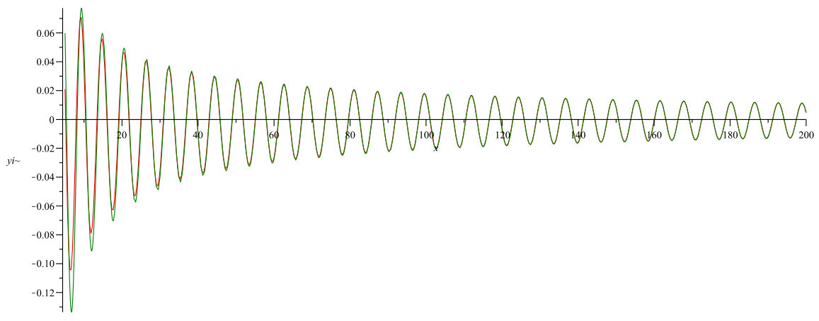 Figure 101
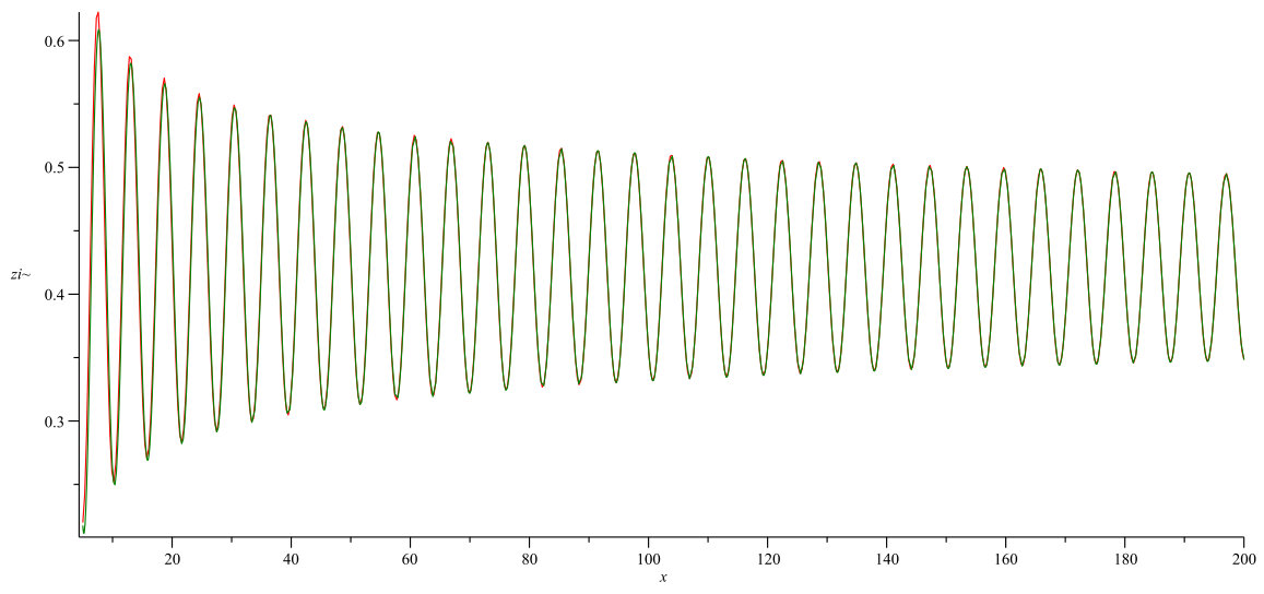 Figure 101
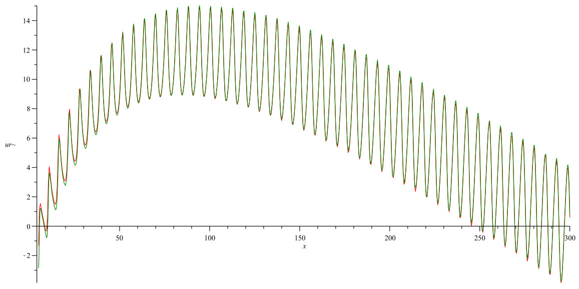 Figure 101
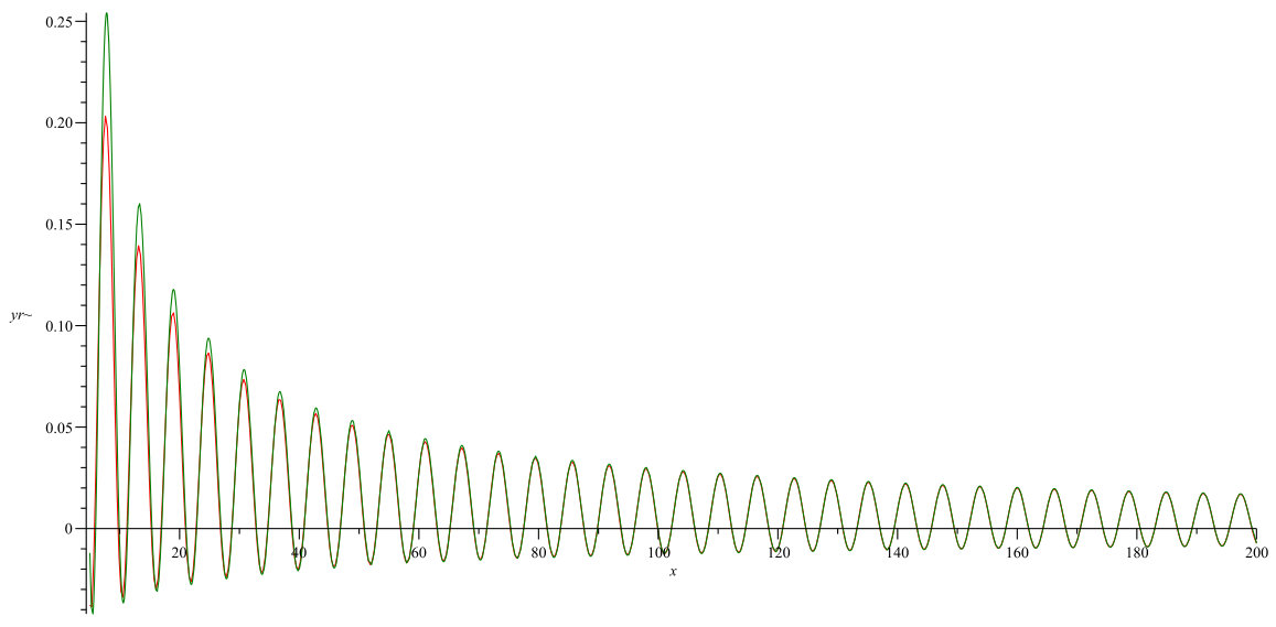 Figure 101
 Figure 101
 Figure 101
 Figure 101
 Figure 101
 Figure 101
 Figure 101
 Figure 101
 Figure 102
 Figure 102
 Figure 102
 Figure 102
 Figure 102
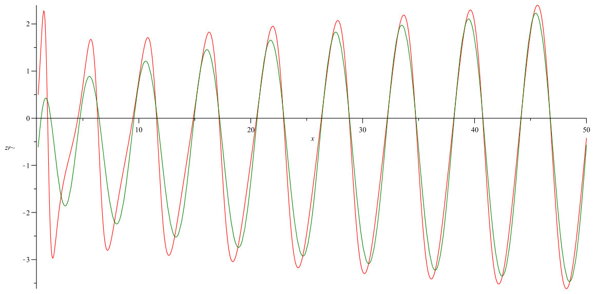 Figure 102
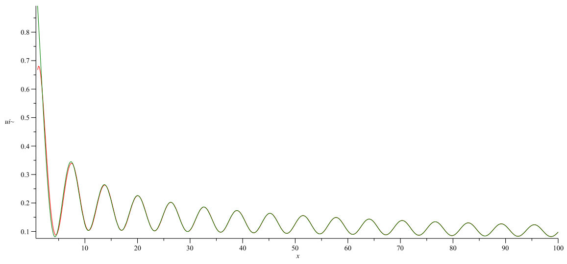 Figure 103
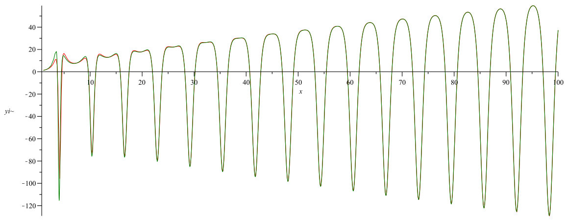 Figure 103
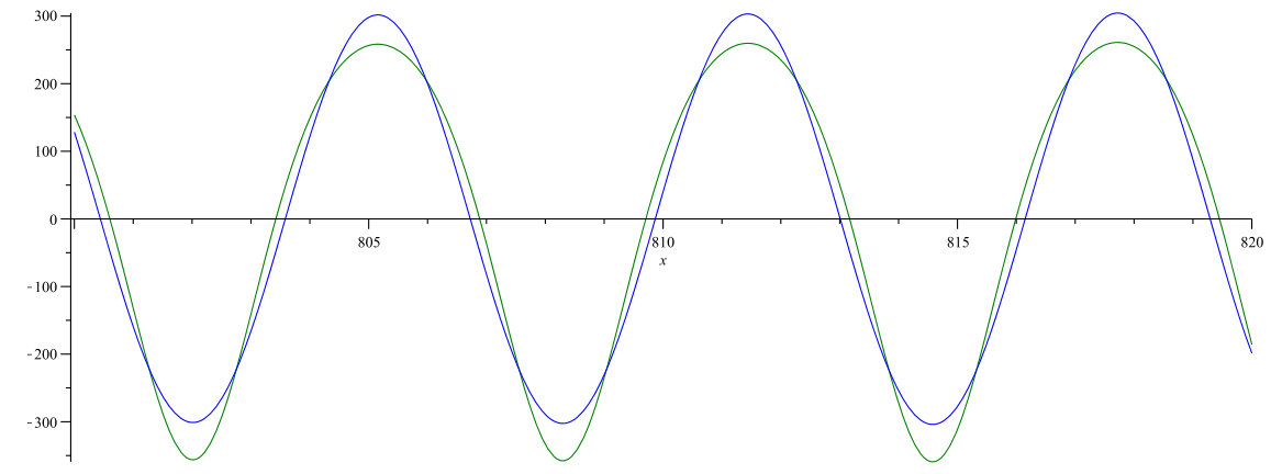 Figure 103
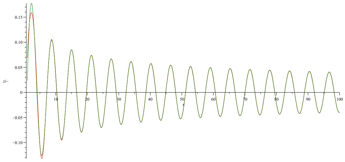 Figure 103
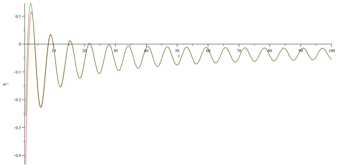 Figure 103
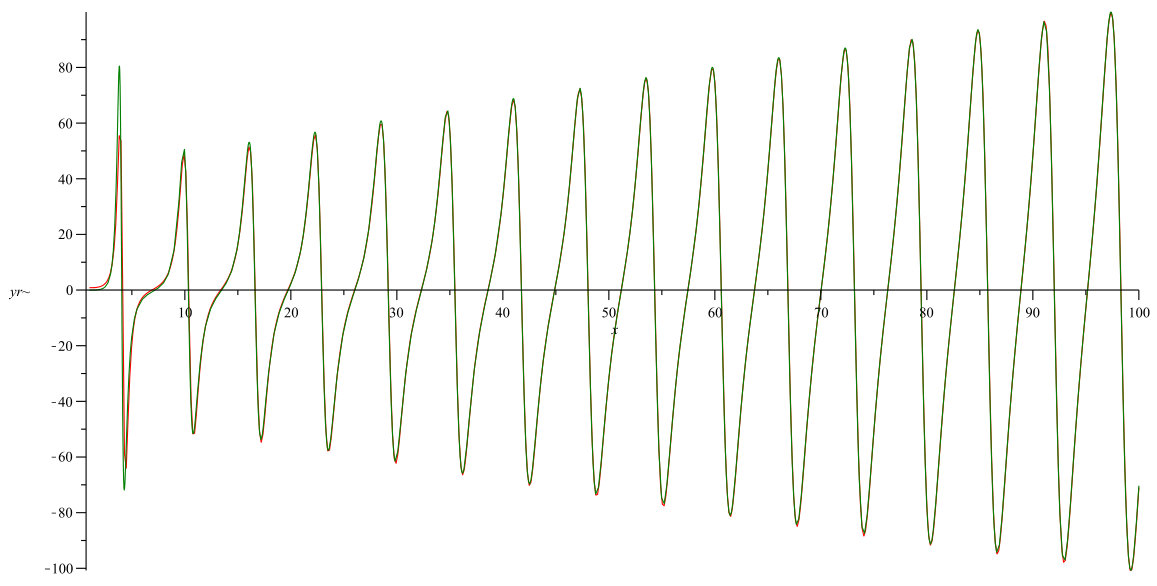 Figure 103
 Figure 103
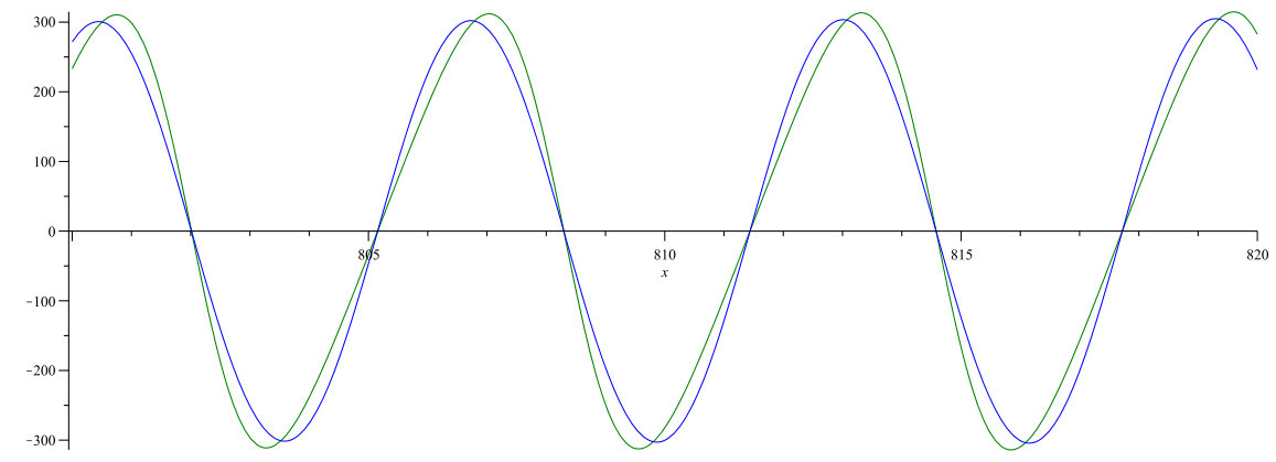 Figure 103
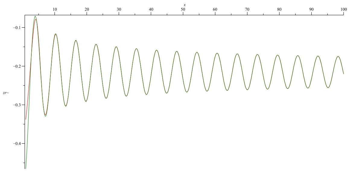 Figure 103
Peer Reviews
No public reviews on file for this paper yet. If you reviewed it on a platform where reviews are public (OpenReview, ICLR, NeurIPS, ICML), you can paste yours below so the community can read it here.
Videos
No videos yet. Explain this paper in a talk, walkthrough, or lecture? Add one.
Taxonomy
TopicsNonlinear Waves and Solitons · Nonlinear Photonic Systems · Quantum chaos and dynamical systems
Connection Formulae for Asymptotics of the
Fifth Painlevé Transcendent on the Imaginary Axis: I
F. V. Andreev and A. V. Kitaev
Department of Mathematics, Western Illinois University, Macomb, IL 61455, USA
Steklov Mathematical Institute, Fontanka 27, St.Petersburg, 191023, Russia E-mail: [email protected]: [email protected]
(April 12, 2019)
Abstract
Leading terms of asymptotic expansions for the general complex solutions of the fifth Painlevé equation as are found. These asymptotics are parameterized by monodromy data of the associated linear ODE,
[TABLE]
The parametrization allows one to derive connection formulas for the asymptotics. We provide numerical verification of the results. Important special cases of the connection formulas are also considered.
2010 Mathematics Subject Classification: 34M55, 33E17, 34M40, 34M35, 34E20.
Key Words: Isomonodromy deformations, Painlevé equations, asymptotics.
Short title: Connection formulas for
1 Introduction
We study asymptotics111The notion “asymptotics” is used throughout the paper to abbreviate the expression “the leading terms of asymptotic expansion” as , , of isomonodromy deformations (with respect to parameter ) of the following linear ODE
[TABLE]
Here \sigma_{3}=\left(\begin{array}[]{cc}1&0\\ 0&-1\end{array}\right) and the matrices () are independent of . This paper is a continuation of our earlier work [1] on asymptotics of the isomonodromy deformations of system (1.1) on the real -axis. For convenience of the reader, we recall here the basic notation and some results obtained in [1].
Following Jimbo and Miwa [12], we consider the following parameterization of the matrices ,
[TABLE]
Then the isomonodromy deformations of Equation (1.1) with respect to are governed by the following system of nonlinear ODEs, which is called the Isomonodromy Deformation System (IDS)
[TABLE]
In this system () are complex constants considered as parameters. Eliminating function from Equation (1.5) by using Equation (1.4), one finds that function satisfies the fifth Painlevé equation :
[TABLE]
Together with the functions , , and , we are also interested in the so-called -function [12, 13, 1]222Function exactly coincides with function introduced by Jimbo and Miwa in [12]., which is associated with the Hamiltonian structure for System (1.4), (1.5) and the corresponding -function. Function , in terms of functions and , is defined as follows
[TABLE]
This function has been proven to be an important object in physical and geometrical applications, where the connection problem for its asymptotics arises in a natural way.
As in the work [1] we use for our studies the method of isomonodromy deformations: this method is based on parametrization of asymptotics of IDS (1.4)-(1.6) via the monodromy data of system (1.1). Such parametrization allows one to find the connection formulae for asymptotics of a given solution at different singular points (in our case [math] and ) and at different directions in the neighborhood of an essential singular point (in our case and ). This parametrization is based on asymptotic solution of the direct and inverse monodromy problems for Equation (1.1). There are various approaches how one can achieve these goals:
(1) Combination of local asymptotic analysis of IDS with the subsequent asymptotic solution of the direct and inverse monodromy problems. Note that IDS can always be presented as the first order system of ODEs with the quadratic r.-h.s. with respect to unknown functions, so that local asymptotics of those systems can be constructed in a regular way. However, the local asymptotic analysis can be also based on various asymptotic ideas and approaches. The following asymptotic solutions of the direct and inverse monodromy problems also can be performed by using slightly different asymptotic methods;
(2) The inverse monodromy problem can be formulated as a matrix Riemann-Hilbert conjugation problem in the complex plane with its further asymptotic solution with the help of the Deift-Zhou asymptotic method;
(3) The method we use here is in general similar to (1), however, it suffers substantial differences. We do not use any apriori information about the local asymptotic expansions for IDS (1.4)-(1.6) or (1.7). Instead, for the solution of the direct monodromy problem for Equation (1.1) some asymptotic assumptions on the matrix elements of of Matrices (1) and (1), which are much less detailed comparing with the local asymptotics, are assumed. These assumptions are dictated by our ability to perform asymptotic estimates which finally lead us to asymptotic solution of the direct monodromy problem. In curse of these calculations appears a number of such assumptions. Then asymptotic solution of the inverse monodromy problem gives us local asymptotics of the matrix elements together with their parameterization via the monodromy data. After that we verify, whether thus obtained asymptotics passes all the assumptions imposed. This verification provide us with the restrictions on monodromy data, for which our analysis is valid. So, this methodology allows one to drop out the preliminary stage of the local asymptotic analysis of IDS. It is substantially based on the fact that we deal with the isomonodromy deformations. We do not touch at any stage of our asymptotic analysis either IDS (1.4)-(1.6), nor Equation (1.7). Therefore, we call this asymptotic method as the Method of Isomonodromy Deformations.
As of now the main source of the connection results for with the normalization on the pure imaginary axis is the papers [7, 8] by McCoy and Tang. In these papers they consider a special case of (1.7) with the parameters and with the primary motivation to serve applications related with the study of correlation functions for the Ising model, level spacing distribution in the theory of random matrices and one-particle density matrix of the one-dimensional impenetrable Bose gas. Methodologically, for studying asymptotics as , these authors applied the scheme (1) outlined above and for asymptotics as used the corresponding results obtained by Jimbo [16]. McCoy and Tang not only proved for the following asymptotics
[TABLE]
where are parameters of the transcendent, but also found the connection formulae for asymptotics of this solution as and .
The case of studied by McCoy and Tang is known to be equivalent to a special case of the third Painlevé equation, so it is not a ”truly” fifth Painlevé transcendent. Our main motivation for this study was to extend the connection results to the case of the true transcendent by following methodology (3) in the above list.
We also study the real reduction of the solutions; this is impossible to get real reduction from solution (1.11).
Recently, two papers devoted to asymptotics on pure imaginary axis were published (see [10] and [11]). In these papers the asymptotics of the general real reduction of the on pure imaginary axis were obtained. These results are in complete agreement with our Corollaries 3.2 and 3.3. Also, in [10] and [11], the general asymptotic of the form
[TABLE]
found by Jimbo in [16], is rigorously and directly proved.
Our results are more advanced than that obtained in [10] and [11] in several aspects. First, we establish the connection formulas which allow one to find the asymptotic parameters at infinity for given parameters in the asymptotic expansion at zero (say, and in the previous formula). This is due to we have computed the monodromy data which is an important result in itself. Second, we found and parameterized asymptotics of the general complex solution, not just real ones. Third, (1.12) is not the only possible solution at zero: there is a lot of others and we give a complete list of them for the case of general -parameters. Finally, our approach is completely different: we use the isomonodromy deformation method (IDM).
Having said this let us note that that the proof of results obtained by IDM can be justified with the help of the scheme suggested in [5]. This scheme requires a more careful attention to error estimates, than that presented in this paper. For the experienced reader it is clear that the estimates possess the properties required for launching the scheme [5]. At the same time the explicit presentation of these estimates would substantially blow up the size of the paper without adding any new information. Since we do not provide all the details we use the word derivation, rather than the proof in the corresponding sections. It is important to mention that there is another possibility of the justification of asymptotics obtained by IDM, it is an application of the well-known Wasow theorem (see Theorem 35.1 of [21]): As long as the leading term of asymptotics is obtained, one can develop it into the complete asymptotic series (see Appendix B), after that the Wasow theorem implies the existence of the solution of IDS with the prescribed asymptotics. In that scheme our derivation constitutes the proof of correspondence between coefficients of the leading terms of asymptotics and monodromy data. The latter proof does not require any special properties of the error estimates and is enough for the justification. Here, however, we do not give the complete details for application of the Wasow theorem, so the word derivation is correct in this sense too.
Although, there are no doubts in the correctness of IDM, surely, there might be some ad hoc faults, in formulae because of the personal reasons, some of them indicated below, we provide our formulae with examples of the numerical verification, which can be useful for he reader interested in application of our results and comparison them with the results obtained by the other authors.
We also refer to the papers [10, 11] mentioned above, which contains rigorous proofs of the asymptotic results, which coincides with special cases of our formulae.
Recently appeared a number of papers [29, 30, 31, 32] where different justification schemes for asymptotics of the fifth Painlevé transcendents has been used. They concern the results for the real axis we discuss in [1], we expect that they will be working for the imaginary axis too.
The paper is organized as follows. In Section 2, we define the monodromy data for Equation (1.1). The main results are presented in Sections 3 and 7, for asymptoics as and , respectively. In Sections 4 and 5 brief derivations of the results, stated in Theorems 3.1 and 3.3, respectively, are presented. In Appendix A, we consider Schlesinger transformations for . Using these Schlesinger transformations, we can derive Theorems 3.2 and 3.3 in an alternative way. In Appendix B, we consider the complete asymptotic series for solutions found in Section 3, and explain how to find the first terms of these series. In Section 6, we compare our results with those obtained in paper [8]. Section 7 is devoted to presentation of the results for small argument, . Comparing to our previous paper we present a refined formula for the leading term of small asymptotics. In Section 8 we deal with the degenerated cases of asymptotics as .
To demonstrate how our results can be used, we consider deriving connection formulas for an equation, we met in applications. Reader can find the details in Section 9.
This paper is written in stylistics close to that of the paper [1] published quite some time ago. This happened because the first draft of this work was written in 1997, soon after preprints [14] and [15] were finished. Paper [1] is the unification of these preprints, which were originally written in different notation. So, after [1] was published in 2000 we turn back to this work to unify notation. Interchanging of the notation required great care and large time because we have got many complicated formulae. We were not able to finish this work at that time because while doing it we digressed to some other studies of the Painlevé equations. We came back to this work only in 2013. Since the large time past after the paper were written and the mess with the notation we decided to check our results independently. On this way appeared Sections 9 and 10 where we considered some special application of our results and undertook numerical studies, respectively. At this stage the paper took the form close to its modern state, however, we again digressed to another studies and were not able to make the final editing. Only after we decided to separate the 1997 draft into two parts we were able to finish the first part in April 2019. The second part of this paper completes asymptotic description of solutions as . It containes one type of asymptotics for general solutions and a few asymptotics for special one parameter families.
It is important to mention that during this time some interesting papers devoted to the study of asymptotics of the fifth Painlevé functions has been published [25, 26, 27, 28].
Acknowledgments. One of the authors (FA) is grateful to Andy Bennett and Lev Kapitanski, Kansas State University, for hospitality and support. His work was partially supported by grants #436–2978 and CMS–9813182.
2 The Manifold of Monodromy Data
In this section, we define the monodromy data [12] for Equation (1.1).
Equation (1.1) has three singular points: irregular one at the infinity and two regular singularities at [math] and . We define the canonical solutions of Equation (1.1) by means of their expansions,
[TABLE]
in the corresponding sectors
[TABLE]
Henceforth, we fix the branch of in the usual way, i.e., , and consider as a given number. For pure imaginary arguments .
The canonical solutions are connected by the so called Stokes matrices,
[TABLE]
Using (2.1), one easily proves that
[TABLE]
Equations (2.3) and (2.4) give us
[TABLE]
Thus, one can determine all the Stokes matrices having two of them. We choose and to be these basic matrices. It follows from Equations (1.1), (2.1), (2.2), and (2.3) that matrices are independent of and of the following structure:
[TABLE]
The complex parameters are called Stokes multipliers. The monodromy matrix at infinity, , for function is defined by the following equation:
[TABLE]
Using Equations (2.3) and (2.4), one finds
[TABLE]
In the following, we use only one of these matrices
[TABLE]
All other matrices can be expressed in terms of via the following recurrence relation
[TABLE]
To deal with monodromy matrices at finite singularities at [math] and we define a single-valued branch of . It is convenient to restrict to the domain . In this domain is a single-valued analytical function (of ) with the following expansions at the regular singularities , :
[TABLE]
We assume here that . If is an integer the expansion is modified as it is written in [14]. The series in Equation (2.10) is convergent for .
Using expansions (2.10), we define the monodromy matrices at the regular singular points as follows:
[TABLE]
Even though expansion (2.10) does not define uniquely, the matrices are defined properly.
The monodromy matrices are connected by the following cyclic relation [16]
[TABLE]
The matrix elements , , Stokes multipliers, , , and the parameters are called the monodromy data of Equation(1.1). It is easy to check that the data satisfy the following relations:
[TABLE]
System. (2.13) in , for fixed define an algebraic variety which is called the manifold of monodromy data, . In terms of , Eqs. (2.13) read as:
[TABLE]
Note that . Given a point in (that is matrices and ), one finds the Stokes multipliers via relations (2.8) and (2.12). Thus, completely defines all the monodromy data.
The given point defines Matrices (1) and (1) that, in its turn, Equation (1.1). A solution to direct monodromy problem is a correspondence
[TABLE]
An inverse map
[TABLE]
where and , is a solution to inverse monodromy problem. If the inverse monodromy problem is solvable, its solution is unique. If we demand that point does not move when we vary , the corresponding solution of the inverse monodromy problem, i.e., functions , , and , are called the isomonodromy deformations, which means that the monodromy data do not change. The main result is that in the case of isomonodromy deformations the functions , , and satisfy Eqs. (1.4)–(1.6) [12].
Only in exceptional cases the direct and/or inverse monodromy problems can be solved explicitly. Therefore, we have to apply asymptotic methods. In this paper we solve the direct monodromy problem asymptotically as with and, also, for . We find asymptotics, parameterized by some complex numbers and present explicit formulas for the monodromy data in terms of these parameters.
3 Results
The asymptotic results formulated in this section are valid in the cheese-like domains, and , in the complex -plane. The subscripts means that the positive, respectively, negative imaginary semiaxes, beginning with some finite point, belong to the corresponding domains. The domains with different subscripts do not intersect, the different superscripts of the domains with the same subscripts means different locations of the holes inside the domains. An important property of these domains is that the solution of System (1.4)–(1.6), the set of functions , , and , as well as their asymptotics restricted in the domains are singlevalued analytic functions. This fact is important for justification of asymptotics as well as the study of distribution of zeroes and poles of the solutions along the imaginary axis.
The precise definition of the domains are given in Theorems 3.1 and 3.2 below, before we specify the branch of function with , which we use in our domains to write our asymptotic formulae. We define on the imaginary axis as for and for and extend it on the entire domains and via the analytic continuation.
Theorem 3.1**.**
Let and , and . Denote
[TABLE]
and assume . Then, for each value of the sign there exists the unique solution of System (1.4)–(1.6)* with the following asymptotic expansion*
[TABLE]
as and with , where
[TABLE]
where the sequences, and , are infinite series of solutions (if they exist) of the equations
[TABLE]
with .
Remark 3.1**.**
The notation and with means that asymptotics hold for all rather large with either or, respectively, . We recall that the functions , , have the branching point at (cf. Section 7) so that it is important to specify the argument of . All error estimates depend on all the parameters: , , , and ’s, including those characterizing the domains : , , and . Exclusion of the negative integer values of and does not follow from our derivation. This requirement is dictated by the justification scheme outlined in the Introduction: in the case of negative integer values of these parameters one cannot uniquely specify the corresponding solution by the monodromy data (cf. Theorem 3.3 and Equations (2.14)–(2.16)). It does not mean that solutions with the corresponding asymptotics do not exist: just our calculation requires a minor modification. More specifically, in this case we have to calculate the other monodromy parameters than that given in Equations (3.4)–(3.5) below. It is important to mention that although Theorems 3.1 and 3.2 do not refer to the monodromy data, our way of proving them is based on the monodromy correspondence established in Theorem 3.3.**
Remark 3.2**.**
It is clear that infinite series of solutions of Equations (3.1) satisfying the condition exist only in the case . Thus, in the case the domain is just a strip along the imaginary axis (”the cheese without holes”) incised along the segment . One can prove that for all rather large in any circle with small enough radius (see definition of ) centred at zeroes of asymptotics, , there exists one and only one zero of the Painlevé function . Therefore solutions described in Theorem 3.1 do not have poles in .**
Remark 3.3**.**
Instead of taking the imaginary axis as the axis of the domain our derivation presented below with little modifications works for a ”logarithmic deformation” of the imaginary axis, namely, for any . In this case instead of we can formulate our result in -neighborhood of the ”deformed imaginary axis”, which can be denoted as . In this case all asymptotics announced in Theorem 3.1 are valid and the condition on should be changed to . In the error estimates one also has to change . It is interesting to note that points of the logarithmic curve satisfy the asymptotic condition in the sense that as .
Because the parameter is arbitrary we can consider slightly more complicated domains, than , where the asymptotics still hold, e.g., if we can write our asymptotics in the -neighborhood of the domain bounded on the right with the logarithmic curve and on the left with the imaginary axis. In this case the parameter is bounded as follows, . We can also consider domains which are bounded on the right and on the left with the logarithmic curves with positive and negative values of the parameter , or with the same sign of in the latter case they would not contain the imaginary axis. These asymptotics in the ”logarithmic” domains allow us to establish existence of infinite sets of zeroes, as , for which logarithmically (with respect to ) moving away from the imaginary axis.**
Theorem 3.2**.**
Let and , and . Denote
[TABLE]
and assume . Then, for each value of the sign there exists the unique solution of System (1.4)–(1.6)* with the following asymptotic expansion*
[TABLE]
as and with , where
[TABLE]
where the sequences, and , are infinite series of solutions (if they exist) of the equations
[TABLE]
with .
Remark 3.4**.**
Remark 3.1 holds with the change . Remark 3.2 is also valid if one replaces: with , with , Theorem 3.1 with Theorem 3.2, and considers zeroes instead of poles. Remark 3.3 also can be reformulated for the results stated in Theorem 3.2 as existence of the infinite sequence of poles , , which diverges from the imaginary axis logarithmically. If we introduce the parameter instead of : , than the range of the validity of the asymptotics in the -deformed domain can be described as , and in the error estimates we must change .**
Remark 3.5**.**
As mentioned at the end of Section 5 and in Subsection 4.6 the results reported in Theorems 3.1 and 3.2 continue to describe the qualitative behavior of function beyond the intervals of validity of the theorems, namely, for , where . The error estimates in Theorem 3.k for the functions and equal and , respectively. Since , then for , we get ; thus Theorem 3.(3-k) gives much better approximation than Theorem 3.k. In the domain where at least one of the parameters satisfies the condition , which can be rewritten in terms of as , the first (largest) terms of asymptotics given by both Theorems 3.1 and 3.2 coincide:
[TABLE]
Corollary 3.1**.**
For solutions defined in Theorems 3.1 and 3.2 the corresponding -function (1.9) has the following asymptotics as , , and :
[TABLE]
Remark 3.6**.**
The parameter in asymptotics (3.3) satisfies the condition . In the case all explicitly written terms in (3.3) larger than the error estimate; if or , then one or, respectively, two terms in the right-hand side of Equation (3.3) are equal or smaller the error estimate and can be neglected.
Theorem 3.3**.**
Solutions of System (1.4)–(1.6) described in Theorems 3.1 and 3.2 define the isomonodromy deformations of Equation (1.1) with the following monodromy data:
[TABLE]
If asymptotic expansions of solutions in these theorems are understood to be given for , then
[TABLE]
if , then
[TABLE]
Corollary 3.2**.**
Denote
[TABLE]
Assume that and as well as the coefficients of Equation (1.7), and , are real and
[TABLE]
Then the solution defined in Theorem 3.1 is real for the pure imaginary values of , namely, , , for , and its asymptotics as and can be rewritten as follows:
[TABLE]
where is the parameter introduced in Theorem 3.1. For real solutions with asymptotics (3.8) is given by the relation
[TABLE]
Corollary 3.3**.**
Denote
[TABLE]
Assume that and as well as the coefficients of Equation (1.7), and , are real and
[TABLE]
Then the solution defined in Theorem 3.2 is real for the pure imaginary values of , namely, , , for , and its asymptotics as and can be rewritten as follows:
[TABLE]
where is the parameter introduced in Theorem 3.1. For real solutions with asymptotics (3.9) is given by the relation
[TABLE]
4 Derivation I
In this Section we asymptotically, as , solve the direct monodromy problem for Equation (1.1) by making several assumptions on asymptotical behavior of its coefficients. First of all, we do all our calculations in the cheese-like strip domain along the imaginary axis. There are two real positive parameters characterizing this domain: the half-width of the strip, , and the radius of its holes, . These parameters are assumed to be fixed in the course of the calculations so that the error estimates depend on these parameters. These holes are assumed to contain possible poles of and , and zeroes of , to avoid problems with the estimates of coefficients of Equation (1.1). The exact location of the centres of these holes are unknown in the ”first round” of our calculations, we assumed only the conditions on the functions and imposed below (4.1) and (4.2). In the ”second round” of calculations we put centres of the holes exactly at zeroes and poles of the leading term of asymptotics which we find at the end of the first round.
The notation more precisely means that we are taking a limit along any path in the cheese-like domain: and . The choice of the path is not important because of the Painlevé property of System (1.4)–(1.5). All our functions of , say, , , etc. are assumed to be analytic continuation from the positive real axis. These functions have only two singular points at [math] and . After we make a cut along the negative real semiaxis the analytic continuations mentioned above are correctly defined. The zeroes and poles of the coefficients of Equation (1.1), if any, can be located only in the holes of the strip domain.
Our main assumptions on the coefficients in this Section are as follows:
[TABLE]
These asymptotic restrictions are assumed to be valid in the closure of the cheese-like domain. We use them in most calculations in this section. Some further restrictions will appear in course of calculations and will be clearly indicated in the corresponding places333 The radius of holes () is fixed as a positive parameter, however it is important to note that this radius can be chosen even merging, \delta_{2}=\mathcal{O}\big{(}t^{-\epsilon\big{)}},0<\epsilon<1/2. We do not use this fact here. Let us explain our convention for the use of the and notation: When we write we actually mean that there exists some and such that , notation with means that .
In this section the direct monodromy problem is solved asymptotically for Equation (1.1) with coefficients in some classes of functions analytic in the cheese-like strip domain and satisfying certain asymptotic conditions. Some of these conditions have a form of simple systems of algebraic equations that can be uniquely resolved to explicitly give the leading terms of asymptotics for the functions. One proves that thus obtained solution satisfies all the other conditions imposed in the process of solving of the direct monodromy problem. Now when we have explicit formulae for asymptotics we can check that all our error estimates smoothly depends on the monodromy parameters. In particular, the estimates hold under small local variations of the monodromy data. Due to the way our asymptotics are obtained and because they are parameterized with the monodromy data, we can say that they represent an asymptotic solution of the inverse monodromy problem.
It is not immediately obvious that any asymptotic solution of the inverse monodromy problem represents an asymptotic expansion of some solution of the system (1.4)–(1.6). However, there is a justification scheme [5] that allows one to prove (exact) solvability of the corresponding monodromy problem as long as its asymptotic solution is obtained via the method explained above.
To simplify the notation we perform the following gauge transformation,
[TABLE]
Then we observe that function satisfies equation (1.1) but with . We will compute the monodromy data for function . For matrices , , with , we use the same notation, . The function will be restored in the final formulae for the monodromy data.
Another convention we follow is that in course of calculations we use notation for function . This function has the following asymptotic evaluation as , , where is a parameter, i.e., independent of and ’s variables. In formulation of the results of solution of the inverse monodromy problem we use a simpler notation in the sense of .
The reader will find below two types of equalities: exact and asymptotic. All asymptotic equalities with respect to in this section are understood as in the cheese-like strip domain; in case an asymptotic equality is understood in some other sense, say, with respect to the latter is explained. We also use notation to indicate asymptotic equalities modulo lesser terms.
4.1 WKB-method
To obtain the monodromy data in terms of parameters of asymptotic expansion for large pure imaginary , we apply the WKB-method.
Let us start from the exact formula for
[TABLE]
where
[TABLE]
In addition to (4.1) and (4.2), we will also suppose that
[TABLE]
Due to this, we may rewrite so that
[TABLE]
The error estimate in Equation (4.7) is valid provided the following redefinition of is made,
[TABLE]
This redefinition is assumed below. It does not effect on the following calculations since we calculate up to the order .
Then, we define
[TABLE]
Clearly this function is defined up to an arbitrary function of , which does not play any role because in the following we consider the definite integral (see Equation (4.16)). It is obvious that there exists function with the following asymptotics as
[TABLE]
provided for and . Here as and as . We need the following asymptotic expansions of function
[TABLE]
To simplify our notation we do not write in Equations (4.10)–(4.12) the -estimate from Equation (4.9), because it does not contribute to the final result, however we have to keep in mind the domain on the -plane where it is valid.
We impose one more condition on the functions and ,
[TABLE]
for some . Condition (4.13) does not neither follow nor contradict conditions (4.1) and (4.2): it means just a special relation between asymptotic values of the functions and . A posteriori we know that , however, at this stage we do not fix it.
Then, in the domain , where and , the following estimate takes place
[TABLE]
The definition of contains the same ambiguity as the one for , so that the comment to Estimate (4.15) is analogous to the one after Equation (4.8).
We use the following representation of WKB-formula ([1])
[TABLE]
where is the so-called Stokes domain (see, e.g. [1]) and is an arbitrary fixed point from . The paths of integration in Equation (4.16) with , , defined in Equations (4.8) and (4.14), should be taken in . Here, however, we do not consider in detail the definition of the Stokes graph, because the turning points in our case coalesce with the singular points and for our purposes we can formulate the result in a simpler way (see Theorem (4.1)).
We fix in such a way that as , . Due to (4.13), the term with is of order and can be ignored.
Let us write the asymptotic expansions we need
[TABLE]
In the region , , we have
[TABLE]
where we impose one more assumption,
[TABLE]
For the large ,
[TABLE]
Hereafter, if two expressions are connected by the symbol “”, then they are equal up to a scalar nonzero multiplier.
Instead of defining the Stokes domains, we formulate the following theorem.
Theorem 4.1**.**
Assume that coefficients of Equation (4.3) satisfy the following conditions: (4.1), (4.2), (4.6), (4.13), and (4.23). Then, for any there exists a solution of Equation (4.3) with the following asymptotic expansion at large pure imaginary ,
[TABLE]
on the ray , , where . Point lies on the same ray.
4.2 A model equation for solutions near the singular points
As usual, the WKB-asymptotic fails near the singular points. In the neighborhood of these points, we need another approximation. To find it, we introduce the model functions . Slightly modified, these functions can be found in [16]. They satisfy the following linear differential equation
[TABLE]
Asymptotic expansions of these solutions in the sectors
[TABLE]
are as follows
[TABLE]
They define the functions uniquely. Following the standard method (see, for instance, [1]), we define the monodromy parameters for Equation (4.26).
The solutions of Equation (4.26) are connected by Stokes matrices
[TABLE]
All the Stokes matrices can be found via and using the relation
[TABLE]
For and we have
[TABLE]
The Stokes multipliers , , are given by explicit formulae:
[TABLE]
We choose function as the “main” basic function. The explicit construction for this function is given by M. Jimbo
[TABLE]
Here is the Whitteker function. The asymptotic expansion as is given as follows
[TABLE]
where
[TABLE]
We introduce the following monodromy matrix
[TABLE]
and find
[TABLE]
Also, we will need another monodromy matrix related to :
[TABLE]
The entry , which we do not use in the following text, can be computed with the help of the relation .
4.3 Singular point
In the neighborhood of the point , we can rewrite Equation (4.3) as
[TABLE]
Divide this equation by and introduce the variable . Then, function satisfies the equation
[TABLE]
We introduce function , which satisfies the equation
[TABLE]
where we used Assumption (4.23) and denoted .
To obtain the basic equation (4.26), we transform the first matrix in the right-hand side of the previous equation to the diagonal form substituting Y^{(2)}=T_{1}Y^{(3)}=\left(\begin{array}[]{cc}1&-\beta_{1}\\ 0&1\end{array}\right)Y^{(3)}. Then, satisfies the following equation
[TABLE]
Here,
[TABLE]
Since
[TABLE]
we see that parameter in the model equation should be taken equal to . Then from the equation on , namely from the diagonal element in , we can find parameter in the model equation:
[TABLE]
So, we know that and in the model equation are and correspondingly, but we still do not have model equation, because . We transform the equation by a diagonal matrix: and find that satisfies the following equation:
[TABLE]
that is the model equation (4.26). Parameter should be taken as follows:
[TABLE]
We also assume that , which is consistent with Theorem 3.1.
Now, the standard proof [6] allows us to formulate the following Theorem.
Theorem 4.2**.**
For any , there exist a solution of Equation with the following asymptotic expansion as
[TABLE]
Corollary 4.1**.**
In the region, , , the asymptotic expansion of function has the following form
[TABLE]
in the sector
[TABLE]
Corollary 4.2**.**
In the region, , the asymptotic expansion of function is given by
[TABLE]
In these statements
[TABLE]
Hereafter, we will understand all multivalued logarithmic functions of in this way.
4.4 Singular point
The construction presented in this subsection is analogous to the one in Subsection 4.3. In particular here we do not arrive at new restrictions on functions and .
In the neighborhood of the point we write down Equation (4.3) as follows,
[TABLE]
We divide this equation by and introduce the variable . Then, function satisfies the equation
[TABLE]
where, .
To obtain the model equation (4.26), we make the substitution
[TABLE]
Then, satisfies the equation
[TABLE]
Here,
[TABLE]
Note that
[TABLE]
and we can find the parameters and in the model equation: and
[TABLE]
with defined in Equation (4.34). Now we map equation on to the model Equation (4.26) by making the following transformation , where
[TABLE]
Then, we find that satisfies the following equation:
[TABLE]
that is exactly the model equation (4.26).
As in Subsection 4.3 we arrive at the following results:
Theorem 4.3**.**
For any , there exist a solution of Equation with the following asymptotic expansion as
[TABLE]
Corollary 4.3**.**
In the region, , , the asymptotic expansion of function is given by
[TABLE]
This asymptotic expansion is valid in the sector
[TABLE]
Corollary 4.4**.**
In the region, , the asymptotic expansion of function is
[TABLE]
4.5 Matching
We have defined the following solutions of Equation (4.3): the canonical solutions,; the solutions with the WKB asymptotics, ; and the solutions in the proper neighbohoods of the singular points, , . Since all of them are solutions of the same equation, the following matrices
[TABLE]
are independent of . Due to Corollaries 4.2 and 4.4,
[TABLE]
where the matrices are also independent of .
Our immediate goal is to find asymptotics of these matrices as . After that, we find asymptotics of the matrices (see Section 2), via the following relation:
[TABLE]
where we restored function (see introductory part for this Section).
For any integer (note that the imaginary unit is denoted as )
[TABLE]
where the error estimate is a diagonal matrix. This estimation is obtained by taking asymptotics as along the corresponding (to ) Stokes line in the second equation (4.43). The error estimate is a diagonal matrix, because the off-diagonal entries would be –dependent.
To find asymptotics of matrices we use their definition (4.43), where we take asymptotics as , , along Stokes lines of the functions . Again we have to take the diagonal part of the asymptotics because the non-trivial off-diagonal part would be -dependent.
Using expansions (4.38) and (4.25), with and given by (4.12) and (4.22), respectively, we want to match these solutions in the leading term. In order for the leading term the leading terms of the matrices not to depend on , the following condition should be valid
[TABLE]
Assuming the above condition is true, one finds,
[TABLE]
where, again, the error term is a diagonal matrix. We find asymptotics of in the similar way, with the help of equations (4.41), (4.25), (4.12), and (4.22). The result reads
[TABLE]
Now we have enough information to calculate all the monodromy data introduced in Section 2. We, however, are going to find a minimal set of the data which completely characterize the domain of the monodromy manifold corresponding to our assumptions on the coefficients of Equation (1.1) which are made in the preceding Subsections.
To simplify further relations, we need some preliminary notation. Denote the upper (p=0) – and lower (p=1) – triangular subgroups of with the unit diagonal,
[TABLE]
where the symbol stands for arbitrary complex number. Subgroup acts on via the right multiplication. We use the same notation for this action, since it cannot cause any misunderstanding. Note that element is not changed by transformation , while element is not changed by .
Let be a diagonal subgroup of . Then, for any and
[TABLE]
By employing this notation, the matrices (see Equation (4.44)) due to Equations (4.36), (4.40), (4.27), and (4.29), can be written as follows:
[TABLE]
Relations (4.46), (4.48), (4.49), (4.51), (4.52), and (4.53) give us information sufficient to find asymptotics of matrices (see (2.10)).
First, consider the case . Then, in the neighborhood of point , we have: for real , . Note that asymptotic expansion of is fixed at . Thus,
[TABLE]
In the neighborhood of point , we have: for real , . Note that: 1) solution is fixed at ; 2) ; 3) matrices are diagonal ones, ; 4) relations (4.52) and (4.50) take place. So,
[TABLE]
Now, consider the case . Then, in the neighborhood of point , we have: for real , . Note that asymptotic expansion of is fixed at . Repeating the arguments above, we have
[TABLE]
In the neighborhood of point , we have: for real , . Note that solution is fixed at . Thus,
[TABLE]
Combining all these facts together, we find
[TABLE]
Note that in Equations (4.54)–(4.57) the error estimates, , are diagonal matrices.
The manifold of monodromy data is three-dimensional. Thus, we are to obtain three parameters in monodromy data. When , we can find two parameters from relation (4.54) and one parameter from (4.55). When , we can find one parameter from relation (4.56) and two parameters from (4.57). In both cases, one of the matrices has the following structure: , where is a diagonal matrix, . So, the diagonal elements of the corresponding monodromy matrix are equal to those from (4.32). Using this remark, we find for :
[TABLE]
For , we have
[TABLE]
Since the monodromy data (4.58) and (4.59) do not depend on , we arrive at the following asymptotic expansions:
[TABLE]
are parameters (independent of ). At this point we recall our notational agreement (see the preamble to Section 4) and consider as a complex parameter, rather than a function of with the behavior as .
Now, substituting the first two conditions (4.60) into Equations (4.58) and (4.59), and taking into account that the matrix elements are independent of , so that we can take the limit , we arrive at the results announced in Theorem 3.3. Let us note that the expressions for and (as functions of , , and ) remain the same regardless of sign of . Only and differ.
4.6 Asymptotics of System (1.4)–(1.6)
To get the results announced in Theorem 3.1, we rewrite the first two Equations (4.60) and the one for , (4.47), in terms of , and , see Equations (4.39), (4.35), and (4.34), respectively:
[TABLE]
Substituting the ratio in the l.-h.s. of Equation (4.61) into Equation (4.63) we obtain a linear algebraic equation for . Solving it we successively obtain and from Equations (4.61) and (4.62), respectively:
[TABLE]
where we denoted
[TABLE]
Thus we get explicit expressions for , , and . The same expressions, presented however in a multiplicative form, are given in Theorem 3.1 as the leading terms of the asymptotic expansions. According to our justification scheme outlined in Introduction to announce these formulae as asymptotics of the true solutions of System (1.4)–(1.6) we have to check that all our assumptions and error estimates made in this section are valid. The latter, in fact, leads to some restrictions on our asymptotic parameters. To find them we note that as :
[TABLE]
Most of the calculations done in this section are valid for , as indicated in the preamble to this Section. However, the matching requires, see Equation (4.47), the following restriction on :
[TABLE]
The left inequality in (4.68) follows from the fact that for negative function is growing . This growth is bounded by the second term in Equation (4.47). Let us explain the right inequality in (4.68). For positive Equation (4.47) implies \varphi_{2}=\mathcal{O}\big{(}t^{\nu_{1}-2}\big{)}+\mathcal{O}\big{(}t^{-1}\big{)}. We demand that the second term in asymptotics of (see Equation (4.65)), which has the order , should be greater than . Otherwise the asymptotics of would consists of only one constant term which contains only one parameter and therefore gives only very rough approximation for this function, in particular, such asymptotics does not uniquely characterize function . At the same time the condition does not improve radically our asymptotics for function , because this asymptotics is mainly defined (see Equation (4.61)) by multiplication of the constant term in asymptotics of with the growing power term \mathcal{O}\big{(}t^{\nu_{1}}\big{)}. Thus, one can continue to use asymptotics of announced in Theorem 3.1 in the region . Our numerical studies (see Section 10) confirms this observation.
Now we are ready to discuss the accuracy of approximation of function by the asymptotics given in Theorem 3.1. This question is intimately related with the error estimate we introduced in (4.61) for function . This estimate allows us to confirm only the largest term in asymptotics of in case . However, as we see below, we can assert that our result gives us up to three correct terms in asymptotics of .
Note that the estimate (in ) defines the class of functions for which we calculate the monodromy data. Our calculations are valid for any estimate in . Therefore, to formulate the best possible asymptotic result for the functions and that follows from our derivation we have to demand that this is as small as possible. It cannot be equal to [math] because in this case Equation (4.61) would provide us with the first integral for general solutions of the system (1.4)–(1.5) which is not possible. At the same time there is no sense to demand that the error estimate for is better than the one for function , since function appeared for the first time in Equation (4.61) in the ratio . Therefore, the order of the error estimate in Theorem 3.1, which follows from our derivation coincides with the order of the estimate related with the transition from function to the parameter (see preamble Section 4). This means that practically we can omit -term in Equation (4.61). Very similar reasoning leads to the conclusion that the error estimate for function in Equations (4.62) and (4.66) can be chosen coinciding with the one for . The latter means that in all Equations (4.64)–(4.66) we can omit terms and take into account the error that comes out from function . The best possible error for transition from function to the parameter which comes from our calculation coincides with . The following analysis is based on this fact.
First consider positive values of . The error estimate for function in this case is \mathcal{O}\big{(}1/t\big{)}, which gives the following error estimate for function in Theorem 3.1,
[TABLE]
Thus, because of the inequality which holds for we see that all three terms of asymptotics of (Equation (4.64) without terms) are larger than the error estimate (4.69). In the case only the two first terms of asymptotics of are larger than the error estimate; we note that in the whole interval two terms of asymptotics are larger than the error estimate for both functions and (see Equations (4.64) and (4.65) with the omitted terms).
The conclusion made in the above paragraph is consistent with the complete asymptotic expansions for functions and developed in Appendix B, namely, one can improve approximation of function by adding up the following correction terms:
[TABLE]
where and are defined in Appendix B.
It is mentioned above that one can continue to use asymptotics of given in Theorem 3.1 in the region . It is worth noting that for the latter values of the error estimate for function is , i.e. is growing, and for it is still vanishing, . It is easy to observe that Theorem 3.2 deliver much better approximation of and, surely, for these values of . At the boundary value , the leading (growing) term of asymptotics of function and the leading (constant) term of asymptotics of given by both Theorems 3.1 and 3.2 coincide. Either result can be used for approximation of these functions: the accuracy (which one is better?) depends on the particular solution. One has to use the correction terms given in Appendix B, especially for approximation of function , to achieve a ”reasonably” good asymptotic description of these functions. The reader will find a numeric example in Subsection 10.4.
Consider now negative values of for general solutions:
[TABLE]
In this case \varphi_{2}=\mathcal{O}\big{(}t^{-2\nu_{1}-1}\big{)}, therefore, the error estimate in both formulae for and in Theorem 3.1 is of the order . Both function and have exactly the same leading term of asymptotics (here we again refer to Equations (4.64) and (4.65)) proportional to . Therefore, in the region all three terms of asymptotics for function and two terms for function are larger than the error estimate. In the case two terms of asymptotics for functions and are larger than the error estimate. Finally, for only the largest terms of asymptotics for and are larger than the corresponding error estimates.
5 Derivation II
In this section we outline some basic steps which lead to Theorem 3.2. The scheme of the proof and major steps of calculations are the same as in the previous section. Therefore here we outline only modifications that are needed for the case under consideration.
The major assumptions on the coefficients of Equation (1.1) are as follows:
[TABLE]
In fact, these conditions are equivalent to those given by Equations (4.1) and (4.2) in Section 4. In this section we continue to use the conventions about symbols and made in the paragraph below Equations (4.1) and (4.2).
Therefore, we do not need to change anything in the WKB-method, except for asymptotics of matrix :
[TABLE]
The reason for this change is the following assumption on the functions and ,
[TABLE]
which we use now instead of Assumption (4.23). For solution in the neighborhood of , we have the same result as above (see Theorem 4.2 and Corollaries 4.1, and 4.2), but now:
[TABLE]
For solution in the neighborhood of the point , we have the same result as above (see Theorem 4.3 and Corollaries 4.3, 4.4), but now:
[TABLE]
The matching goes exactly as before. In particular, for matrices and we get exactly the same expressions (4.48) and (4.49), respectively, but with and defined in (5.4) and (5.5). Proceeding exactly as in Section 4, we arrive at formulas (4.58) and (4.59) for the monodromy data.
Next, we introduce asymptotic parameters, and by formulae (4.60), with the corresponding parameters and .
The asymptotic parameter is defined in Equation (4.5). However, due to the conditions (5.1), Equation (4.47) should be changed to
[TABLE]
Now, using definitions for and , (5.4) and (5.5), and condition (5.6), we can write an analog of system (4.61)–(4.63):
[TABLE]
where
[TABLE]
Opening the parenthesis in Equations (5.7) and (5.9) and substituting the term in Equation (5.9) by its expression obtained from Equation (5.7) one finds
[TABLE]
Here we include the error estimate from Equation (5.9) into the notation as agreed in preamble of Section 4. Substituting given by Equation (5.10) into Equation (5.8) we get the leading term of asymptotics for function in Theorem 3.2. Making the same substitution into Equation (5.7) we obtain
[TABLE]
Now factoring out from the parentheses in Equation (5.11) the term we get the leading term of asymptotics for presented in Theorem 3.2. Substituting the latter asymptotics into Equation (5.10) we obtain asymptotics for . Finally, asymptotics for immeditely follows from Equations (5.8) and (5.10). Thus the analog of System (4.64)–(4.66) reads:
[TABLE]
Reasoning similar to the one presented in Subsection 4.6 shows that to find the best error estimate that comes from our derivation we can put all -estimates in the above formulae to be of the same order as (see (5.6)). Therefore, we have to come back to the error estimate hidden in . The analysis, which is very similar to the one at the end of Section 4 for the parameter , implies similar restriction for the parameter ,
[TABLE]
We can make a comment analogous to the one at the end of Section 4: since asymptotics of is growing in the region the leading term of asymptotics for is still satisfactory, although the asymptotics for given in Theorem 3.1 works better. The situation is worse for function because only the constant term of asymptotics remains larger than the error estimate for . So in the domain , one has to use the result given in Theorem 3.1. In case, either Theorem can be used but to get a good approximation one has to employ the correction terms (see Appendix B).
6 Comparison with the results by McCoy and Tang
In this section, we compare our results with the ones obtained in paper [8]. The authors of [8] considered the case , . We discuss here only the principal case , since the case can be treated as application of the Bäcklund transformations (see Theorem A.1) to the principal one. In particular, the monodromy matrices for coincide with those for . McCoy and Tang obtained the following asymptotic expansion as and ():
[TABLE]
In paper [8] two parameters and are used. In [7, 8] parameter , whereas we fix (see Equation (1.7)). We use notation , instead of in [7, 8], because in Section 10 we denote for . There is an obvious relation , which should be used in the comparison of our results with those obtained in [7, 8]. In Equations (6.1) and (6.2) we simplify the notation by using only the parameter . These results agree with our asymptotic expansions providing the asymptotic parameters are related as
[TABLE]
where .
Now we turn to parametrization of the asymptotics by the monodromy data. In [8] McCoy and Tang expressed the monodromy data in terms of the parameters , which in our notation are defined as follows,
[TABLE]
where is a canonical solution of Equation (1.1) and , is the -element of the monodromy matrix, , corresponding to the singular point . While analyzing their paper [9] devoted to the connection formulae for asymptotics of solutions on the real axis, we observed in [1] that the monodromy parameter was calculated for solution (in our notation), while the parameter was given for . The same remark concerns the imaginary case considered in [8]. By using the formulae presented in Section 2 one finds that in terms of our monodromy data the parameters are given by the following expression:
[TABLE]
The parameters as calculated by McCoy and Tang (see Equations (2.53) and (2.68) in [8]) are:
[TABLE]
Substituting into Equation (6.5) (for ) given by Equation (3.7) and taking into account the first equation (6.3) we see the complete agreement of our results with equation (6.6).
The parameter is more complicated: By making use of Equation (2.16) and the results for the monodromy data presented in Theorem 3.3, we rewrite our monodromy parameter as follows:
[TABLE]
Now, Equation (6.5) (for ) allows us to present the monodromy parameter in the following way:
[TABLE]
In its turn, Equations (6.7) and (6.8) obtained for by McCoy and Tang ([MT]) can be rewritten with the help of relations (6.3) and the well-known identities for the Gamma-function in terms of :
[TABLE]
So, for we have an agreement only up to the sign of or, equivalently, the sign of the parameter or function . If we are to keep the sign of unchanged, then to get we can alternatively demand that either , or , which is equivalent (we recall that ) to one of the following conditions:
[TABLE]
Thus, contrary to the case of real argument , where our parametrization of the quantities and , after being associated to the canonical solutions and , respectively, coincides with the parametrization obtained by McCoy and Tang (see [1]), for pure imaginary these parameterizations coincide only up to the sign of in .
Finally, we comment on the connection formulae for the asymptotics. To get the connection formulae McCoy and Tang employ asymptotics of the fifth Painlevé transcendent as obtained by Jimbo in [16]. The latter asymptotics were parameterized by the monodromy data of the canonical solution in our notation (see Section 2). Thus asymptotics as and in [8] appear to be parameterized by the monodromy data of , and , respectively. Hence, the connection formulae obtained by McCoy and Tang could be correct only in a special situation when all three canonical solutions coincide, , or, in other words, the Stokes multipliers vanish, . Since it means that the monodromy matrix and the corresponding monodromy group of Equation (1.1) is commutative. For their connection formulae on the pure imaginary axis to be correct one should additionally demand one of the conditions (6.10) or (6.11).
In Subsection 10.3 we consider a numerical solution of IDS (1.4)-(1.6) corresponding to nontrivial Stokes multipliers, , , and observe a good agreement with our connection results, while the connection formulae by McCoy and Tang do not show the correct asymptotic behavior.
7 Asymptotic expansions for
In this section is fixed in the standard way, in particular, for . Moreover, is assumed to be bounded as . Let be a complex number. It will be convenient to use the following notations:
[TABLE]
Theorem 7.1**.**
Let and . Let also . Then there exists the unique solution of System (1.4)–(1.5) with the following asymptotic expansion as :
[TABLE]
Corollary 7.1**.**
Function , corresponding to the solution of System (1.4)–(1.6) defined in Theorem 7.1, has the following asymptotic expansion as :
[TABLE]
Remark 7.1**.**
If , then the asymptotic expansion for function can be rewritten as follows:
[TABLE]
Remark 7.2**.**
Small -expansion of the -function related to as,
[TABLE]
has been obtained by Jimbo [16]. We independently derived our results by a similar but slightly different method and presented it in terms of the functions , , , and in [1]. The latter result, together with the asymptotics at infinity, allows one to find the connection formulae for function , that cannot be obtained from Jimbo’s result. The present form of small t-asymptotics (Theorem 7.1) we announced in paper [2], however the error estimates in that paper were correctly written only for . In this paper we have added additional error estimates (see the last terms in Equations (7.2) and (7.3)) which work for the interval . Now the estimates cover the whole semi-open interval, . The origin of this mistake is not related with the isomonodromy deformation method which gives only the leading terms of the asymptotics together with the error estimates in the form \mathcal{O}\big{(}t^{1+\delta}\big{)}, , without specification of the dependence of on . Formally, these estimates looks similar to the first error estimates in Equations (7.2) and (7.3). The explicit form (in terms of ) of these ”isomonodromy error estimates” are obtained via substitution of the corresponding asymptotic expansions into the isomonodromy deformation system (1.4) and (1.5) where the terms important for the parameter in the interval , the last estimates in Equations (7.2) and (7.3), were just overlooked although they have the required form \mathcal{O}\big{(}t^{1+\delta}\big{)}. **
Theorem 7.2**.**
Assume . Then the solution of System (1.4)–(1.6) defined in Theorem 7.1 generates an isomonodromy deformation of Equation (1.1) with the following monodromy data:
[TABLE]
[TABLE]
In the previous formulas:
[TABLE]
Remark 7.3**.**
Multiplying expressions for the Stokes multipliers and in (7.7) one finds
[TABLE]
This equation means that to define parameter for all monodromy data we have to allow .
The case and with , modulo some restrictions on the parameters where , and is served by Theorems 7.1 and 7.2.
The case and the restrictions mentioned in the previous sentence are studied in part II of this work.
We finish this section by considering the case with certain restrictions on the parameters and .
Theorem 7.3**.**
Let . Let also and . Then there exists a solution of system (1.4)–(1.5) with the following asymptotic expansion as :
[TABLE]
Here , , and .
Corollary 7.2**.**
Function , corresponding to the solution of system (1.4)–(1.6) defined in the Theorem 7.3, has the following asymptotic expansion as :
[TABLE]
Theorem 7.4**.**
The solution of system (1.4)–(1.6) described in Theorem 7.3 defines isomonodromy deformation of Equation (1.1) with the following monodromy data:
[TABLE]
[TABLE]
Here
[TABLE]
Remark 7.4**.**
The results stated in the last two theorems can be obtained by the repetition of the calculation scheme outlined in our previous paper [1], but with the asymptotics of the special functions involved there corresponding to the case . Instead, we, following Jimbo (see [16]), consider the limit by making the following substitution, where , in the results stated in Theorems 7.1, Corollary 7.1, and 7.2, respectively. Strictly speaking, to make the results obtained in Theorem 7.3 and Corollary 7.2 via this limiting procedure rigorous, we have to study the dependence of the error estimates in Theorem 7.1 and Corollary 7.1 not only as but also as . Concerning the latter estimates no details are given neither in Jimbo’s paper, nor in our work [1]. Our result is based on the conjecture that the limit of the -th term in the small -expansion of the -function, (the inner sum), can be estimated as . In principle, we do not need to prove this conjecture in case we use the derivation of the results stated in Theorems 7.3, Corollary 7.2 via the ”first principles”. The limiting procedure is simpler in the sense of derivation, but requires a proof of the additional nontrivial result. The limiting procedure in the monodromy data of Theorem 7.2 is the straightforward application of the l’Hopitale rule which is formulated as Theorem 7.4.
Remark 7.5**.**
Jimbo in [16], presented small- asymptotics of only in terms of the -function (see Equation (7.6)) our asymptotic formulae in terms of the functions , , , and are equivalent (with the same comment about as in Remark 7.2) to Jimbo’s one. To see this we have to make one more calculation, because Jimbo didn’t write explicitly the monodromy matrices, like we do in Theorems 7.4 and 7.2, instead he presented the analogs of our matrices (see Section 2) modulo left and right diagonal multipliers. So, below we give some details which explain how one can get Jimbo’s monodromy for .
To obtain this monodromy data (corresponding to the case ), we use formulas for from our previous paper (see [1], Section 10, page 1834):
[TABLE]
where is a diagonal matrix independent of . Let us note that (up to scalar multiplier). To apply the l’Hopitale rule, we need to compute the first derivative of with respect to
[TABLE]
Here and in the list of formulae below, the prime denotes the derivative with respect to taken at . Moreover, all objects that are functions of are assumed taken at , e.g.: , (see Remark 7.4), etc:
[TABLE]
where function is defined in the second equation (7.10) and
[TABLE]
Using the well-known identities for function (see [4]):
[TABLE]
we arrive at the following expressions for the matrices at :
[TABLE]
Now, writing as and putting the matrix elements of and to common denominators, then getting rid of these denominators by factorizing with the help of left and right diagonal matrices such that the numerators do not change, and, finally, omitting the left diagonal matrices (as they do not effect the monodromy matrices) one arrives at the following expressions for the corresponding matrix elements:
[TABLE]
[TABLE]
here matrices coincide with for , respectively, modulo left diagonal factors. Parameter is given in the last equation of (7.9), the sign of is not important, since the monodromy matrices (see Theorem 7.4) depend on . The formulae for exactly coincide with the corresponding matrices obtained by Jimbo [16] modulo the scalar multiplier , which is not given in the paper [16].
8 Degeneration in the general formulas for asymptotics as
Here we show how short- asymptotics of some known particular solutions can be obtained with the help of the results presented in Section 7. We discuss in this section some limiting procedures when two or more parameters simultaneously and consistently tends to some singular points of the formulae presented in the previous section. The parameters which limits we consider parameterize both the monodromy data and the asymptotics of the corresponding solutions. The formulae for the monodromy data are explicit so that the limiting procedures are chosen such that the limiting set of the monodromy data exists. This set of the monodromy data define a solution of IDS (1.4)–(1.6). This statement follows from the justification scheme for asymptotics obtained by the isomonodromy deformation method [5], which can be applied for the large- asymptotics. Then these solutions can be analytically continued into the neighborhood of and so we can discuss their asymptotics as . In our derivation of the results in Section 7 we didn’t study the dependence of the asymptotic estimates as the functions of the parameters which we are going to send to some limiting values. Therefore, there appears a question concerning their behavior in these limits. In fact, it is clear that these estimates cannot be unbounded because it would mean existence of a singularity for all rather small which cannot be the case because of the Painlevé property. The only problem that may occur in the limiting procedure with the small- asymptotics is that the error estimates may become equal or larger than the leading term. In the last case, we cannot get a definite asymptotics directly from our results. In this section we consider only the situations when the leading term of asymptotics after the limiting procedure is larger than the error estimate. In following Section 9 we consider a case when in the limiting procedure the order of the error estimate in the limit coincide with the order of the leading term.
The parameters which are not involved in the limiting procedure are assumed to take general values, i.e., such values that all functions and expressions with these parameters are properly defined at these values.
Note that asymptotic expansions of functions and monodromy data in the theorems of Section 7 are not changed under the formal substitution
[TABLE]
Due to this invariance, we introduce parameters better suited for the change :
[TABLE]
In these notations, the substitution (8.1) can be written as:
[TABLE]
When we formulated our main monodromy results for we excluded the cases when , , or . In this section we outline how one could overcome this difficulty and cover the part of the manifold of monodromy data where these assumptions fail.
Our approach is to: a) explain the cases when functions , or become zeroes and then b) use the results on the Schlesinger transformations to reduce the cases of integer , or to the case when one of these linear combinations is zero. Let us look at asymptotic expansions of functions , , and in Theorem 7.1. These expansions can become degenerate in the following cases:
, 2. 2.
, 3. 3.
.
Degeneration with , , or can be reduced to the previous case, using transformation (8.1). Now we will specify what we mean by degeneration. We define the three types of complete degeneration:
1c
, ,
2c
, , ,
3c
, ,
and the three types of partial degeneration:
1p
, , ,
2p
, , ,
3p
, , .
In the partial degenerations we arrange the limiting procedure such that the finite limits of the rations in the items above exist.
Theorem 8.1**.**
The following monodromy data correspond to complete degeneration 1c and 2c:
[TABLE]
Parameter is defined by equation or depending on degeneration scheme 1c or 2c, respectively.
Corollary 8.1**.**
Let . There exists a solution of system (1.4)–(1.6) with the following asymptotics as :
[TABLE]
The monodromy data from Theorem 8.1 with , degeneration 1c, correspond to this solution.
Corollary 8.2**.**
Let . There exists a solution of system (1.4)–(1.6) with the following asymptotics as :
[TABLE]
The monodromy data from (8.1) with , degeneration 2c, correspond to this solution.
Before concidering degeneration 3c we find partial degeneration 3p.
Corollary 8.3**.**
There exists a solution of system (1.4)–(1.5) with the following asymptotic expansion as :
[TABLE]
The following monodromy data corresponds to this solution
[TABLE]
Here and is the same as in Theorem 7.2. The Stokes multipliers are as follows:
[TABLE]
The previous formulas were obtained in the following way. Let us denote
[TABLE]
Make limit transition as in formulas for functions and . Replace with the adjusted parameter introduced in the beginning of the section. Then, we obtain formulae for function . Make the same substitution in the monodromy data and perform the limit transition. As a result, we arrive to the formulae above.
Remark 8.1**.**
The partial degeneration gives a similar result but with and .
Remark 8.2**.**
Partial degenerations 1p and 2p is easy to obtain just by looking at formulae given in Theorems 7.1 and 7.2. Introduce parameters: or , respectively, and make a limit . We leave this analysis as a simple exercise for the readers.
Now to get complete degeneration case 3c we have to make the following limit in the results presented in Corollary 8.3
[TABLE]
Corollary 8.4**.**
There exists a solution of system (1.4)–(1.5) with the following asymptotic expansion as :
[TABLE]
The following monodromy data corresponds to this solution
[TABLE]
Here is the same as in Theorem 7.2. Both Stokes multipliers in this case vanish, .
Remark 8.3**.**
We recall that in basic Theorems 7.1 and 7.2 the real part of parameter belongs to the semi-interval . Therefore, in the resultas obtained above we have the corresponding restrictions on the parameters ’s. Say, in Corollary 8.4 put , thus . If we consider another complete degeneration, , then we find the same formulae but . In Section 9 we consider in detail the case , . For the general values of the result of Corollary 8.4 can be extended with the help of the Bäcklund trnasformations considered in Appendix A. Analogous comments apply to Corollaries 8.1 and 8.2.
Remark 8.4**.**
Functions and obtained in Corollaries 8.1, 8.2, and 8.4 are regular at and the correction term is evaluated as . In fact all these solutions are holomorphic at , so that the corresponding solutions of System (1.4)–(1.5) are meromorphic functions. We omit a detailed proof of this statement because these solutions were studied in paper [19].
Now we outline the second step of our approach to finding the asymptotic behavior of solutions for parameters satisfying the conditions: , , and . These special cases can be characterized in terms of the Stokes multipliers:
, 2. 2.
, 3. 3.
.
Above we considered the cases , , and . It is already mentioned in Remark 8.3 that the case can be treated with the help of application to asymptotics for the Bäclund transformations considered in Appendix A. These transformations shift by even integers which means an arbitrary integer shift of . It is well-known that analogous transformation is easy to write for and , which generate an integer shift of and together with the corresponding asymptotics.
8.1 Case and
Theorem 8.2**.**
Let and , There exists a solution of system (1.4)–(1.6) with the following asymptotic expansion as
[TABLE]
Here
[TABLE]
Asymptotic expansion of function as is given by the following formula:
[TABLE]
The corresponding monodromy data are given by formulas from Theorem 7.2, where parameters are
[TABLE]
Remark 8.5**.**
Function , corresponding to solution of system (1.4)–(1.6), described in Theorem 8.2, has the following asymptotics as
[TABLE]
Theorem 8.3**.**
Let . Then, there exists a solution of system (1.4)–(1.5) with the following asymptotics as
[TABLE]
where
[TABLE]
Asymptotic expansion of function as is given by the following formula:
[TABLE]
Remark 8.6**.**
Function , corresponding to solution of system (1.4)–(1.6), described in Theorem 8.2, has the following asymptotics as
[TABLE]
Let us briefly describe the derivation of Theorems 8.2 and 8.3. Theorem 8.2 gives us, in particular, case , . Theorem 8.3 corresponds to the case . It is easy to see that , , with and sufficiently small give valid asymptotic expansion for system (1.4)–(1.5). For and we have the following system:
[TABLE]
There are three types of solutions of this system:
a rational function of , where ; 2. 2.
a rational function of ; 3. 3.
a fixed point, that is .
Theorem 8.2 corresponds to case 1), Theorem 8.3 corresponds to case 2), and Theorem 8.5 (see below) corresponds to case 3).
The monodromy data were obtained as follows. It is easy to see that formulas from Theorem 7.2 are not degenerate when , . So we can use them for solutions described in Theorems 8.2 and 8.3. The only thing to find is parameter . However, it can be easily seen that formulas from Theorem 8.2 become formulas from Theorem 7.2, if we put , . Therefore, formulas from Theorem 8.2 are valid in interval . Then, to achieve the correspondence with function from Theorem 7.1, parameters and should be connected as it is stated in Theorem 8.2.
To write the monodromy data for (), we need the following notations
[TABLE]
Theorem 8.4**.**
Solution of system (1.4)–(1.6), defined in Theorem 8.3, generates the following monodromy data
[TABLE]
Here
[TABLE]
So, the matrices are given. The monodromy matrices can be found from their definition:
[TABLE]
Theorem 8.5**.**
There exists solution of system (1.4)–(1.5) with the following asymptotics as
[TABLE]
Monodromy data from Theorem 7.2, with , correspond to this solution.
Theorem 8.5 can be derived as follows. Let us put and tend in formulas from Theorem 8.2. Let us note that this solution was already described among the special solutions above.
9 Special Meromorphic Solution
As an illustration of how one can use the results for monodromy data to derive the connection formula, we consider an example. The example will also clarify how the degeneration procedure, discussed in the previous section, can be performed in particular cases.
In this section we assume that the coefficients of Equation (1.7) are fixed as follows:
[TABLE]
There is a quadratic auto transformation of Equation (1.7) which maps these coefficients into the following ones:
[TABLE]
This equation can be also mapped into the complete third Painlevé equation (see, e.g., [20]).
Proposition 9.1**.**
For any and there exists the unique solution of Equation (1.7) with the following asymptotics as ,
[TABLE]
In fact the solution is holomorphic in some neighborhood of , so that Expansion (9.2) is nothing but the Taylor series. The proof can be done in a straightforward way: substitution of the Expansion (9.2) into Equation (1.7) to obtain the recurrence relations for the coefficients . Then one observes that the recurrence allows one to uniquely present as the polynomials of the first coefficient . Then the Wasow theorem provide us with the existence of the solution. The further analysis of the recurrence relation allows one to prove convergence of Expansion (9.2), which also implies the uniqueness.
Let us mention some properties of Solution (9.2). We also consider the corresponding Taylor expansion of function :
[TABLE]
the coefficients for are polynomials of .
Remark 9.1**.**
We do not write explicitly expansion for function , see Equation (1.9), because it can be easily obtained via Equation (1.10) by integration of Expansion (9.3). The constant of integration is .
Properties of Expansions (9.2) and (9.3) depend on parity of the number :
If is even, then is even (as the function of ), so that for all . The function is neither odd nor even, however, the first odd coefficients also vanish for . Note that .
If is odd, then for , while . The corresponding function is an odd function of , i.e., for all .
If we put , then . It is the simplest rational solution of Equation (1.7). It is known [22] that all rational solutions with the asymptotics as can be obtained from this elementary solution via application of the Bäcklund transformations. Some of these solutions has at the Taylor expansion of the form (9.2), however, in these cases the coefficients of Equation (1.7) differ from (9.1). As follows from [22] is the only case when Solution (9.2) is rational.
An interesting question is whether Solution (9.2) is a truly transcendental Painlevé function in the sense of Umemura (see [23]). For Equation (1.7) this question was analysed in [24]. However, these results are not formulated in terms of the Expansion (9.2) and therefore require additional investigation.
There are a few different ways of how to choose parameters corresponding to coefficients (9.1), see Equations (1.8). Our choice is
[TABLE]
As follows from [24] for even there are no classical solutions, apart from the trivial one . So, we consider the odd values of . If , then ; so that we can put in System (1.4), (1.5) and find as a solution of the Riccati equation. After that we have to check whether there is a solution of the Riccati equation with Expansion (9.2) at . Omitting elementary details we find that such solution exists and is unique,
[TABLE]
here for is the modified Bessel function of the first kind [33]. Solution (9.5) has the following Taylor expansion at ,
[TABLE]
Comparing it with Expansion (9.2) we find .
To proceed further we have to apply to Solution (9.5) the second Bäcklund transformation given in Theorem A.1 (see Appendix A). In this way, by mathematical induction, we find that for all odd there exists only one classical solution of System (1.4), (1.5), which can be presented explicitly in terms of the modified Bessel functions with the Taylor Expansion (9.2). In particular,
[TABLE]
Corresponding values of the parameters , .
Conjecture 9.1**.**
Solution (9.2) with odd is classical iff .
The corresponding monodromy matrices are upper triangular and can be calculated with the help of Section 8.
Because of the restriction , see Sections 7 and Subsection 8.1, we cannot directly apply our results to Solution (9.2) for general . However, as we show below, the case is tractable with the help of Sections 7, 8 and Appendix B. The general case of odd can be further treated with the help of the Bäcklund transformations, see Appendix A. As for the even values of they also can be studied within the framework presented in this paper but with the help of a different ”initial solution”. The case of is interesting in view of applications, however, it goes far beyond our goals in this paper and will be considered elsewhere.
In fact, even in the case solutions show different behavior as depending on the value of . For the illustrative purposes we choose the case . The reader can find numeric illustration of the theoretical results obtained in this section in Subsection 10.4. With the help of Maple Code we can be more specific about the asymptotic expansion at of the main object of our study in this section:
[TABLE]
One can notice that the first terms in this expansion are negative. So it rises a natural question: whether all coefficients of this expansion are negative? The following Statement can be confirmed by mathematical induction applied to the recurrence relation for coefficients obtained via substitution of Expansion (9.2) into Equation (1.7).
Statement 9.1**.**
All polynomials have real coefficients. For large values of these polynomials have the following asymptotics as :
[TABLE]
Consider
[TABLE]
The largest root of this polynomial is
[TABLE]
Numerical studies suggest the following
Conjecture 9.2**.**
All zeroes of all polynomials lie inside the circle of radius centered at the origin of the complex plain.
This conjecture together with Statement 9.1 implies that for real all coefficients of Expansion (9.2) are negative, while for their signs alternate.
Remark 9.2**.**
Define a mapping of the sequence into the set , say, the minus sign goes to [math] and the plus sign to . Denote this sequence of zeroes and ones as . Then our result can be formulated as follows: for , for and , . It is an interesting problem to study the sequences for . For example, in the ”integrable” case, , the corresponding sequence is periodic with the minimal period .
9.1 Monodromy data
Here we calculate the monodromy data for defined by Equation (9.6). Comparing the general asymptotic behavior of as (7.2) with Expansion (9.2) we see that the only possibility to get it is to consider a limit . The functions defining Asymptotics (7.2) for our choice of -parameters (9.4) read:
[TABLE]
Therefore, we see that , . These conditions show that here we meet much ”deeper” degeneration procedure rather than that considered in Section 8. It suggests that it is more reliable to do the direct degeneration of the results presented in the main Theorems 7.1 and 7.2, rather than further degeneration of the results of Section 8. In the intermediate degenerations considered in this section it was assumed that the conditions , , and do not hold simultaneously.
Before making the limit procedure we recall that first we have to:
- freeze in Equations (7.2)–(7.3);
- choose -parameters according to Equations (9.4); and
- make the limit transition .
Since we see that the only way we can achieve it is to send parameter . More carefully examining the limit, we find that in fact we have to assume that
[TABLE]
where the parameter is a complex number. After this assumption Equations (7.2)–(7.3) imply:
[TABLE]
We put as the estimate for because we know small- expansion of the -function obtained by Jimbo [16]. The estimate , can be traced from the corresponding term in the expansion of the -function, see Equations (7.6) and (1.10). This term contains the factor in the denominator. After two differentiations, this term gains an additional factor , so that the factor kills this term in the limit. This mechanism is analogous to disappearance of the explicitly written term (see Equation (7.3)) of the order . Since we know that Solution (9.2) is the only solution with the property , then in fact is given by (9.3) with .
Now we perform the limit in the formulas for the monodromy data given in Theorem 7.2. Performing the limit in Equations (7.7) with the help of relations for given in (9.7) and from (9.8), we see that the Stokes multipliers vanish,
[TABLE]
Further we calculate the limits for the monodromy matrices. For the intermediate matrices we find . This, together with Conditions (9.9) imply:
[TABLE]
The matrix elements
[TABLE]
where . This completes calculation of the monodromy data.
Now we have to find how the monodromy data relate to the Taylor expansion of at . Equations (9.8) do not allow us to find it. We can perform the limit more carefully and find that:
[TABLE]
All the estimates above depend on and . Our purpose is to put . Why would the last two estimates remain finite at this limit? If they (one of them) would blow up, then it means that the monodromy data (9.11) does not correspond to any solution of P5. On the other hand, from the derivation of asymptotics at the point of infinity we know that there is a solution of P5 corresponding to these monodromy data.
The last estimate looks ”dangerous”, since in the limit it may contribute to the second term of asymptotics. So, in fact, the -dependence of the last estimate requires further investigations. This estimate can be obtained explicitly in two ways, either directly from Equation (1.7) or via Equation (1.5) and with the help of asymptotics for the function . Another way is the direct calculation of the monodromy data for this solution via Equation (1.1).
Since all these calculations looks cumbersome, we probably present them somewhere, here we announce the correct result and suggest an indirect proof.
Proposition 9.2**.**
[TABLE]
Proof.
Note that and depend on the parameter whilst functions and do not. So, may depend only on the quadratic combination, . Thus should be an entire function of . On the other hand, the inverse function also should be an entire function. It means (see Theorem 4.3 of [34]), that , where and are some constants. For we have , see Corollary 3 and Proposition 3 (item (1)) of [3]. Thus . In the case , the monodromy matrices are diagonal which implies , see the last two Equations (9.11). Our case corresponds to the lower triangular case: , , of Equation (1.1), the other one corresponds to the upper triangular: , . The monodromy element, say, in our case is defined by the monodromy of the function and equals , in the upper triangular case is defined by the monodromy of the function , which is . Using this fact we arrive at Equation (9.12). ∎
In Subsection 10.4 we provide a numeric evidence of Equation (9.12). For for Solution (9.6) with . The key monodromy data for this solution are as follows:
[TABLE]
9.2 Asymptotics as
Since we have explicit formulae for solution for parameter (see Equation (9.5)), we begin with the asymptotics for this case:
[TABLE]
where , , , . In general is a sequence of positive integers counting the number of Feynman diagrams in a problem in quantum electrodynamics (see sequence A005412 of [35]). The series is divergent,
[TABLE]
The complete asymptotic expansion can be written as a transseries with exponentially small terms. The estimate above can be obtained with the help of this expansion.
Here, to give an instructive example we consider only the case of . Obviously, for the real values of our solution is real for real . In this subsection we apply the results obtained in paper [14]. In that paper asymptotics as of solutions were parameterized via auxiliary parameters and . We use general formulae, Equations (3.5) of [14], and substitute there our particular monodromy data obtained in Subsection 9.1:
[TABLE]
We see that if parameters and are defined uniquely in terms of the initial data , where the branch of is fixed in a natural way: . In terms of , parameter is fixed up to a sign which causes no problem because asymptotics are invariant under this change. In this case we have to use the results reported in Theorems 3.1 and 3.2 of [14]. In particular, it means that our solution is regular on the real positive semiaxis and the asymptotics of functions and the reader can find in Theorem 3.1. Theorem 3.2 gives us the asymptotics of the corresponding function .
Consider the case in a more detail. First we have to choose the real part of so that one of the Theorems 3.1 or 4.1 would be applicable. It fixes uniquely parameter as follows,
[TABLE]
This equation implies that we are in the situation described by Theorem 4.1 of [14]. It means that in this case our solution has infinite number of poles on the positive semiaxis. According to Theorem 4.1 function has the following asymptotics in the proper cheese-like domain,
[TABLE]
where
[TABLE]
The last equality holds because the quantity under the logarithm is unimodular. The reader can find the corresponding asymptotics of function and in Theorem 4.1 and Corollary 4.1 of [14], respectively.
The numeric values for the parameters and corresponding to Solution (9.6) (with ) are as follows:
[TABLE]
9.3 Transform
Since general solutions of System (1.4)–(1.6) are not singlevalued, transformation should be considered for analytic continuation of functions , , and for , for all . However, the solution we are interested in is a very special one, and is in fact singlevalued, we consider only the case . Here we present formulae which are valid for the general solution of System (1.4)–(1.6). The purpose of this transformation is that the analytic continuation of any solution at the point can be presented in terms of another solution of this system at the original point . To uniquely define the latter solution we consider action of this transformation not only on the space of the solutions but also on the manifold of monodromy data.
We refer to the definition of the canonical solutions given in Section 2, but here we use an extended notation to reflect their dependence on the coefficients of Equation (1.1). As one can easily see, transform induces the following transformation of the canonical solutions:
[TABLE]
where , , and
[TABLE]
The monodromy data are transformed as follows:
[TABLE]
There is another transformation for IDS (1.4) -(1.6):
[TABLE]
The corresponding transformation of the monodromy data can be found with the help of the following transformation for the canonical solutions:
[TABLE]
Here we assumed that
[TABLE]
The other tilde-variables are defined in Equations (9.19). Equation (9.20) imply the following relation for the monodromy data:
[TABLE]
For our solution (see Equations (9.10)) we have so that for . This is consistent with the fact that Solution (9.2)
[TABLE]
The last equality holds because of the relation . Thus functions and are just the analytic continuation of and and, therefore have the same monodromy data.
9.4 Asymptotics as
Here we apply the first transformation considered in the previous subsection to find asymptotics of solution (9.2) as . The monodromy data for our solution are given in Equations (9.9) and (9.11). Using Equations (9.18) we find that
[TABLE]
In particular we have for . On the other hand
[TABLE]
So, the functions and coincide for all arguments, but have different monodromy data! It is explained by the fact that , therefore the corresponding functions and are different. It is solutions of IDS (1.4)–(1.6), rather than solutions of Equation (1.7), which are characterized uniquely by the monodromy data.
Now consider . Using Asymptotics (9.13) we find,
[TABLE]
where the asymptotic expansion is of the same type as (9.13). It is given by a divergent series, all numbers , are positive integers representing sequence A094664 of [35] with the following asymptotics,
[TABLE]
The complete expansion can be presented as transeries with exponentially small terms. In fact, our calculation represent an explicit relation between sequences A005412 A094664 of [35] which possibly was not observed earlier.
Turning to the general value of the initial data , we note that
[TABLE]
where and are the parameters defined for the solution , , and via Equations (9.14) and (9.15) with the corresponding monodromy data. Since these parameters define asymptotic behaviour of our solution we conclude that qualitatively on the negative semiaxis the solution behaves similar to on the positive one.
Explicit asymptotics for can be found with the help of Theorems 3.1 and 3.2 of [14]. In the case the asymptotics is given in Theorem 4.1 of [14]. For example, in the last case,
[TABLE]
where and are given by Equations (9.16). For the numerical values of and for see (9.17).
9.5 Asymptotics for pure imaginary
With the help of explicit formula (9.5) one finds:
[TABLE]
Consider now the asymptotics as for the general initial data . We see from (9.12) that . Theorem 3.3 implies:
[TABLE]
With the help of the duplication formula for the gamma function we can rewrite as follows,
[TABLE]
Both parameters and introduced in Theorems 3.1 and 3.2 satisfy the condition , which is the boundary value for their applicability. It was mentioned in Remark 3.5 that in fact these theorems are valid beyond these boundary values. In this case we can apply either Theorem for construction of the asymptotics. Suppose we consider Theorem 3.1. Numerics presented in Subsection 10.4 show that the leading term (see Theorem 3.1) delivers quite satisfactory approximation of the function . So the terms are not needed, at least, for description of the qualitative behavior of . At the same time the leading term of in this case is just a constant, therefore even for understanding of the qualitative behavior of we need the the terms .
In our case () asymptotics presented in Theorem 3.1 does not allow one to get -terms correctly for both functions and . The result presented there contains some -terms but not all the terms of this order. To get these terms we included Appendix B, where we presented the complete asymptotic expansions for , , and for large pure imaginary corresponding to both Theorems 3.1 and 3.2. Following a notation introduced in Appendix B we denote,
[TABLE]
For we have . Putting we rewrite in terms of ,
[TABLE]
Substituting the values for -parameters into Equations (B.4) and (B.5) we arrive at the following asymptotics:
[TABLE]
We also present these asymptotics in terms of -variables:
[TABLE]
The last asymptotics reflects the fact that for pure imaginary : and .
Asymptotics of for (9.28) coincides with (9.21). We recall that in this case , which is consistent with (9.29).
Numerical values for :
[TABLE]
Now consider asymptotics for the negative imaginary axis (). Asymptotics for in this case can be calculated via the symmetry considered in Subsection 9.3, since our special solution does not depend on the sign of . However, the corresponding function depends on this sign. Therefore, to get asymptotics in this case we again address Theorems 3.1 and 3.3 and Appendix B. To distinguish from the previous case we denote basic parameters as and . Then Theorem 3.3 implies:
[TABLE]
Here denotes complex conjugation of the parameter . Parameter is given by Equation (9.24) but with , therefore .
The conditions on parameters and in Theorems 3.1 and 3.2, respectively, do not depend on the imaginary part of , so we conclude that asymptotics of functions and z(t) as are given by r.-h.s. of Equations (9.26) and (9.26) with and , where is defined by Equation (9.25) with and . Turning to -variables we have to put , then and asymptotics of functions and as are given by the complex conjugation of Equations (9.28) and (9.29), respectively.
10 Numerical Verification
The purpose of this section is twofold: 1) To check the absence of any occasional mistakes in the formulae presented in this paper, and 2) To visualize solutions of the fifth Painlevé equation and related functions.
The results of our numerical verifications are presented on figures. In the online version of the paper, graphs of numerical solutions are given in red colors while graphs of their large- asymptotics are plotted in green. In the early version of the paper the numerical calculations were done with the help of MATHEMATICA code. In this version we redid these calculations with MAPLE code for the purpose of presenting additionally the connection results for function , which were absent before. Inclusion of makes verification more complete. This function appears also in some applications and helps to calculate asymptotics of some interesting integrals with functions and . On the newly produced figures we presented the plots on intervals closer to the origin, so that the reader can see when the functions achieve their asymptotic behavior.
In this section we use the following notation:
[TABLE]
Assuming that argument of is fixed as above we denote
[TABLE]
In numerical calculations we choose the point in the neighborhood of , where we take initial data, for the numeric calculation of the solution under investigation. The solution is defined by taking some particular values for parameters , , and , defining asymptotic behavior of solutions as , see Section 7. Using asymptotics presented in Theorem 7.1 we calculate the corresponding initial data. Thus it is clear that the closer to the origin the better initial data correspond to the chosen parameters. On the other hand the closer to the origin the more precision is required in the calculations, which increases the time of calculations. The reader can notice that choice of varies between computations, which is done intentionally. For some solutions to get a reliable result we have to choose the initial point by a factor closer to the origin, than for some others. So the choice of is an important issue in the calculations. In all examples presented in this section parameter is chosen with some margin for error. It means that making it 5–10 times larger wouldn’t result in a visible change of the graphs. Similarly, making it smaller also does not have a noticeable visual effect on the plots (while certainly changing slightly the numerical values).
Note that for the solution considered in Subsection 10.4 we used a different scheme of calculations which allows for to be zero.
We conclude the introductory part of this section by giving some details on settings for MAPLE and Mathematica codes we used.
In MAPLE code for most of the calculations the value of parameter Digits 10–14 is enough. The word ‘enough’ in the previous sentence means that by making smaller and increasing the accuracy of calculations we cannot notice any visual change in the plots. For producing of the pictures we set this parameter to 16. We used the standard dsolve procedure with parameters and . For plotting we used procedure with . The increase of accuracy with the help of these parameters does not effect any how on visual quality of the plots though may results in substantial increase of the time of calculations.
The original plots were produced with MATHEMATICA code. In the process of numerically solving the ODE we have to use arbitrary-precision arithmetic. We solve System (1.4), (1.5) via NDSolve command with parameters WorkingPrecision at 40 and MaxSteps set to Infinity. As explained in documentation on NDSolve, the parameters PrecisionGoal and AccuracyGoal are set to half of WorkingPrecision by default. Thus, in our case they are set to 20. We have to specify the terminal, or final, point . For calculations with such accuracy in most cases after we were not able to distinguish the plots of the numerical solutions and their large- asymptotics. So that we used markers on the curves to show that it is actually two curves rather than one.
In presentation of numerical values we give only the first 9 digits after the decimal point. In fact, as follows from above we have done our calculations with the better accuracy. In case a numerical value of some parameter is given with a less amounts of digits it means that it is its exact value.
10.1 Generic Case: Theorem 3.1,
In this subsection we present two examples of solutions whose asymptotics on positive imaginary semi-axis can be constructed with the help of Theorem 3.1.
For our first numerical run we fix the formal monodromies as follows:
[TABLE]
and take the parameters defining asymptotics as as follows
[TABLE]
We use the leading terms of asymptotics given in Theorem 7.1 to calculate the initial data for the numerical solutions at :
[TABLE]
To calculate the parameters and defining, according Theorems 3.1 and 3.2, the large- asymptotics of the functions and we have first to find the monodromy data with the help of Theorem 7.2. According to Theorem 3.3 we need only the following data:
[TABLE]
Now, Theorem 3.3 implies:
[TABLE]
Note that by Theorem 3.3 (see Equation (3.6)) is defined via logarithms. Namely, is defined . To fix it uniquely we have to calculate parameters and given in Theorems 3.1 and 3.2:
[TABLE]
and check whether one of the numbers , , fits the interval . In our case fits the interval, while does not. If neither number is within the interval, we have, using the ambiguity in , to adjust one of them to fit the interval . If such adjustment is not possible for a given value of , then the reader is addressed to part II of this work.
In our case we are in conditions of Theorem 3.1. So that the large- asymptotics have to be calculated with the help of this Theorem.
The results of the calculations (with ) are presented on Figs. 1-6. The range of calculations on all figures was from to . Since qualitative large- behavior of functions and is obvious from Figures 1-4, we bounded the range of the plot by . Function shows a more interesting behavior so we plotted it on the whole range it was calculated.
Now we consider the second case. Since the scheme of calculations is exactly the same we present only numerical values of the parameters and the resulting graphs.
[TABLE]
Initial values for the numerical solution:
[TABLE]
The monodromy data:
[TABLE]
The parameters of asymptotics as :
[TABLE]
The parameters are as follows:
[TABLE]
which implies that we have to use again Theorem 3.1. The results of calculations () are presented on Figs. 7-12. Here we plotted the solutions on a small segment , to show how the large- asymptotics approximate the solution at finite interval. The settings indicated in preamble to this section allows one to plot the solutions far beyond . On Figures 11-12 we see that function has poles approaching the positive imaginary semi-axis as .
10.2 Generic case: ,
In this subsection we check our asymptotic results for the case when the real part of one of the formal monodromies is greater than . In most cases this situation can be served (at least formally) with the help of the symmetry groups acting in the space of solutions of IDS (1.4)–(1.6). Therefore, it is enough to restrict real parts of formal monodromies within the segment . Such type of restrictions very often are imposed in studies of the Painlevé equations. However, application of the symmetries to asymptotics is often related with cumbersome calculations. Moreover, sometimes in these calculations it is not enough to deal only with the leading term of the asymptotics, because the corresponding terms may cancel, so that one has to keep a few minor terms in asymptotic expansion to get the correct result. At the same time none of our results includes this limitation on the real parts of the formal monodromies. Therefore, it is reasonable to demonstrate the validity of our asymptotic results in the situation beyond the limitations on real parts of the formal monodromies.
The set of formal monodromies for this subsection is as follows:
[TABLE]
The choice of the parameters defining asymptotics as is the same as in the first example of the previous subsection:
[TABLE]
It is an experimental fact that the construction of the numerical solution with the scheme explained in preamble of this section requires to take the initial point closer to the origin, namely, . Note that in this case variable is defined as .
The initial values of the numerical solution:
[TABLE]
The monodromy data of the solution reads:
[TABLE]
The parameters defining asymptotics as are as follows:
[TABLE]
As follows from Equation (10.2) we are within the conditions of Theorem 3.2. Note that parameter here is calculated via Equation (3.7). The corresponding asymptotic and numerical solutions are plotted on the Figs. 13-18.
The accuracy of calculations (see the preamble to this section) allows one to build plot of the numerical solution which visually coincides with its large- asymptotics far beyond . Specifically, we present plots on segment , where the reader still can see difference between the numerical solution and the asymptotics.
10.3 Numerical Illustration to Section 6
In Section 6 we compared our formulae with those obtained in [7, 8]. Here we consider a particular example with both non vanishing Stokes multipliers.
The formal monodromies in this subsection are as follows:
[TABLE]
Here we choose asymptotic parameters in a different way comparing to the previous subsections, namely,
[TABLE]
The first parameter defines branching of the solution at the second one - branching of the solution at the point at infinity. As in Subsection 10.2 consider the negative imaginary semi-axis, with . Theorem 3.3 implies that the parameter determines
[TABLE]
In the case with the help of the same theorem one calculates monodromy parameter . Next, Theorem 7.2 shows that the parameter defining the solution of IDS (1.4)–(1.5) as can be determined as a solution of a quadratic equation, which means that in the generic situation (including our case) there are two solutions with parameters (10.3). We choose one of these solutions
[TABLE]
We started with resulting in initial conditions
[TABLE]
Parameters , and with the help of Theorem 7.2 allow one to find all the monodromy data:
[TABLE]
Thus, actually, both Stokes multipliers do not vanish.
Now, using Theorem 3.3, we find
[TABLE]
Finally, we calculate parameters and (see Theorems 3.1 and 3.2):
[TABLE]
Thus we see that we are within the applicability of Theorem 3.2. The results of comparison of the numerical and large- asymptotics for functions: , , and with are presented on Figs. 19–24. On these figures we compare numerical solution with its large- asymptotics on the segment . As usual we ensure that the accuracy in initial data for numerical solution is such that its plot visually coincides with the plot of asymptotics on the distances far beyond .
Now, we consider the connection formulae for asymptotics which are obtained in [7, 8].
As mentioned in Section 6 our results may coincide in some important particular cases, specifically when , and, at least, one of the Stokes multipliers or vanishes. For the complete match of all connection results both Stokes multipliers should vanish, . In the last case there is no difference between solutions , , and , then we observe an agreement between our results and those of [7, 8]. In particular, a solution of Equation (1.7), describing the one-particle reduced density matrix of the one-dimensional impenetrable Bose gas [17], belongs to this special case.
As follows from Equation (7.8) if one of the Stokes multipliers vanishes, then . For the solution considered in this subsection (see Equation (10.3)), therefore our asymptotic predictions will disagree with those following from papers [7, 8].
In paper [8] the connection formulae are given in terms of the monodromy data, like in our work. In paper [7] the connection formulae are presented directly: the parameters of asymptotics at infinity are given in terms of the parameters of asymptotics as . We tried both types of the connection formulae.
We begin with the connection formulae presented in [8]. In Section 6 we explained that the authors of [8] parameterise the large- asymptotics () in terms of the quantities which are related with the monodromy data via Equation (6.4). We use the definition of the monodromy data given in Section 2 and obtained the following expressions for the Stokes multipliers in terms of :
[TABLE]
[TABLE]
[TABLE]
[TABLE]
For the case , , studied in [7]-[8], they simplify to:
[TABLE]
For the particular numerical case studied here Equation (6.4) implies:
[TABLE]
Substituting these values into Equation (10.5) with we find
[TABLE]
which confirms the values of the Stokes multipliers (10.4) calculated directly.
It is worth reminding that for connection formulae, if we want to remain within the results of [7]-[9], the parameters should be (in our notation) adjusted as explained in Section 6 (see Equation (6.5)). With parameters understood in that way we would find:
[TABLE]
Calculating the Stokes multipliers with the help of and via (10.5) with we get
[TABLE]
As expected, we obtain different Stokes multipliers.
To get the large- asymptotics as suggested in [8] we have to calculate parameters and (see Section 6) Equations (6.6)–(6.8). First we do it with the help of and :
[TABLE]
The plot of the large- asymptotics corresponding to these parameters calculated with the help of Equation (6.2) is presented on Figure 25. Comparing this plot with the ones presented on Figure 19 we see the main discrepancy is that the function on Figure 25 is decaying while it should grow.
We also tried in this case the direct connection formulae given in [7] (see Equations (2.3) and (2.14)–(2.17) of [7]). We applied the scheme of calculations adopted in this paper: first with the help of the initial value found above ( and ) we calculated, with the help of Equation (2.3) of [7], the parameter , then parameters and by means of Equations (2.14)–(2.17)of [7]. Thus obtained and differ with and obtained above. Nevertheless, the qualitative behavior of asymptotics is the same as on Figure 25. The difference in the values of the parameters could be explained because our small- asymptotics, being formally equivalent to the one used in [7], in fact, in most cases numerically is more precise. It is not an obstacle in usage of Equation (2.3) of [7], but the point for calculation of initial value should be chosen closer to the origin, which may require a higher precision of calculations.
We also calculated the plots of asymptotics of for parameters and . In this case asymptotic parameters are as follows:
[TABLE]
We have further (pure experimentally) adjusted parameter , namely, we changed . On Figures 26 and 27 we compared asymptotics of [8], adjusted as explained above, with the ones presented in this work. In the online version our asymptotics colored in green while those of [7] are blue. At first glance, asymptotics for looks quite satisfactory, while for there is some discrepancy which also does not look fatal. Because one may hope that the higher order terms may further correct the situation. However, as we see above our asymptotic formulae from Theorems 3.1 and 3.2, gives good numeric approximations starting from quite small values of ; Asymptotics (6.2) works at these values of not that good. We compared the solutions on the interval and observed significant disagreement between adjusted solutions from [7] and the numerical results. Of course, the interval may not be asymptotically ”large enough” yet. Therefore, we compared asymptotics in segment where they are supposed to coincide (visually) with the numerical solution. At least with the growth of both curves should approach each other. However, the difference between the curves looks ”stable” with variation of within the range . This corresponds with what is written in Section 6. As explained in Section 6, the adjustment suggested there does not repair the situation, one have to put zero at least one of the Stokes multiplier. So, Figures 26 and 27 provide us an illustration to the conclusions of Section 6.
10.4 The Special Meromorphic Solution
In this subsection we deal with the solution studied in Section 9. Since it is a very special solution we have here an opportunity to to choose a different numeric scheme and not the one used in previous subsections. We put , with . We also assume . Then the second transformation in Subsection 9.3 implies:
[TABLE]
where the bar denotes complex conjugation. We recall that and , therefore we make the following change of variables:
[TABLE]
where and are realvalued functions of real variable .
Taking into account that and we rewrite System (1.4), (1.5) as follows:
[TABLE]
The main difference in numeric calculation of this solution comparing with the previous examples is that we can take the initial condition exactly at :
[TABLE]
On Figures 28 and 29 we present the plots of real and imaginary parts of solution for , respectively. Each figure contains two plots: the numerical plot and asymptotic one. To plot asymptotics of we use only the leading term denoted as , see Equation (9.25) in Subsection 9.5. We see that the leading term of the large -asymptotics gives already a very good approximation as early as . A rather remarkable property of that example is that there is no visible transition interval from the behavior of at to its large -behavior.
Since the leading asymptotic term of is a constant we used the explicit form of the oscillating correction term (), to compare it with the numerical solution on Figure 30.
Appendix A Appendix: Schlesinger transformations
Here for completeness we present the Schlesinger transformations of Equation (1.1) together with the corresponding Bäcklund transformations of IDS (1.4)-(1.6), which we use in this paper.
We denote , , the canonical solution of Equation (1.1) corresponding to the set of variables , the notation states for the canonical solution of Equation (1.1) but with variables: . The Schlesinger transformation maps to such that both solutions have the same monodromy data, except the formal monodromy at the point at infinity which is shifted by . Due to these properties the Schlesinger transformations are called sometimes the discrete isomonodromy transformations.
In transformation presented below in Theorem A.1 the original non-tilde variables might be arbitrary. In that case the tilde variables represent just a covariant transformation of Equation (1.1). As long as we require dependence of the tilde variables on , such that they satisfy IDS (1.4)-(1.6), the corresponding monodromy data are independent of (continuous isomonodromy deformations). Obviously, in that case the monodromy data for are also independent of , so that the Schlesinger transformations generate the so-called Bäcklund transformations for solutions of IDS (1.4)-(1.6), i.e., the discrete and continuous isomonodromy flows commute.
Theorem A.1**.**
There exists the following Schlesinger transformation of Equation (1.1)
[TABLE]
where and are the corresponding elements of matrices and , respectively, defined for the non-tilde variables.
[TABLE]
There exists the following inverse Schlesinger transformation of Equation (1.1)
[TABLE]
[TABLE]
Appendix B Appendix: Higher order terms in asymptotic expansion
We begin with the complete asymptotic expansions at large pure imaginary corresponding to solutions of System (1.4)–(1.5) described in Theorem 3.1. The first expansion reads:
[TABLE]
These are the formal (divergent) series with coefficients uniquely determined by substitution into System (1.4)–(1.5) under a recurrence procedure. Below, the reader will find the first terms corresponding to which we found with the help of MATHEMATICA code. This formal expansion becomes asymptotic one provided , where is introduced in Theorem 3.1.
The justification of these asymptotics can be obtained with the help of the scheme described in Section 33 of [21]. The major difference is that the sector where our expansions are valid has the vanishing angle (parameter in [21]). This fact, however, does not destroy the proof because of Remark 3.3, where we explain that, in fact, asymptotics is working in domains rather than only on the imaginary axis. Therefore, in case there exists a solution of System (1.4)–(1.5) with Asymptotics (B.1)–(B.2). Since according to Theorem 3.3 parameter uniquely defines the solution of System (1.4)–(1.5), the solution which exists by the application of the Wasow scheme coincides with the one that described by the monodromy theory and there is no any other solution with the same asymptotic expansion.
We find the coefficients of this asymptotic expansion to be:
[TABLE]
[TABLE]
[TABLE]
[TABLE]
[TABLE]
Substituting the above formulae into Equation (1.9) we find the following result,
[TABLE]
which is formulated in Corollary 3.1. Up to the equality
[TABLE]
is satisfied.
The leading term of asymptotics in Theorem 3.1 is valid also for negative values of . The corresponding asymptotic expansion can be constructed as follows. Define
[TABLE]
Consider the formal series:
[TABLE]
where is the integer part of a number (the integer floor). One proves that these series are asymptotic as , iff . Comparing Equations (B.3) and (B.6) we see that . Substituting this relation into Series (B.7) and (B.8), it is easy to observe that after a rearrangement of terms they coincide with Series (B.1) and (B.2), respectively. Any partial sum of Series (B.1) or (B.2) can be presented as a partial sum of the corresponding Series (B.7) or (B.8) with some extra higher order terms and vice versa so that both pairs of series solve IDS (1.4) and (1.5). So, Series (B.7) and (B.8) represent asymptotics of the same solution as Series (B.1) and (B.2) but in a shifted domain of the parameter : . We discuss this expansion in a more detail in part II of this paper.
For the solutions defined in Theorem 3.2 we have to write another asymptotic expansions. Define
[TABLE]
then for such that , the following formal series are asymptotic:
[TABLE]
For we have to use asymptotic expansion analogous to (B.1) and (B.2):
[TABLE]
The reference list from the paper itself. Each links out to its DOI / PubMed record.
- 1[1] F. V. Andreev and A. V. Kitaev, Connection formulas for asymptotics of the fifth Painlevé transcendent on the real axis, Nonlinearity 13 , no. 5, 1801–1840 (2000).
- 2[2] F. V. Andreev and A. V. Kitaev, On connection formulas for the asymptotics of some special solutions of the fifth Painlevé equation, (Russian) Zap. Nauchn. Sem. POMI 243 , 117–127 (1997); English translation in J. Math. Sci. (New York) 99 , no.1, 808–815 (2000).
- 3[3] F. V. Andreev and A. V. Kitaev, Exponentially small corrections to divergent asymptotic expansions of solutions of the fifth Painlevé equation, Math. Res. Lett. 4 , no. 5, 741–759 (1997).
- 4[4] A. Erdélyi, W. Magnus, F. Oberhettinger, F. G. Tricomi, Higher Transcendental Functions , I ( Bateman Manuscript Project. ), New York-Toronto-London: Mc Graw-Hill Book Company Co. Inc., (1953).
- 5[5] A. V. Kitaev, The justification of asymptotic formulas that can be obtained by the method of isomonodromic deformations, (Russian), Zap. Nauchn. Sem. Leningrad. Otdel. Mat. Inst. Steklov. (LOMI) 179 (1989),101–109; English translation in J. Soviet Math. 57 (1991), no. 3, 3131–3135.
- 6[6] W. Wasow, Asymptotic expansions for ordinary differential equations, Dover Publications, New York, 1987.
- 7[7] B. M. Mc Coy and Sh. Tang, Connection formulae for Painlevé functions , Physica 18D , 190–196 (1986).
- 8[8] B. M. Mc Coy and Sh. Tang, Connection formulae for Painlevé V functions II. The δ 𝛿 \delta function Bose gase problem , Physica 20D , 187–216 (1986).