Lower Bounds for the Bandwidth Problem
Franz Rendl, Renata Sotirov, Christian Truden

TL;DR
This paper introduces a new method using vertex partitions and semidefinite programming to derive lower bounds for the graph bandwidth problem, improving the trade-off between bound quality and computational efficiency.
Contribution
It presents a novel approach that generalizes previous bounds and incorporates SDP relaxation for better lower bounds on graph bandwidth.
Findings
The approach generalizes existing bounds.
Semidefinite programming improves bound accuracy.
Effective on real-world graph instances.
Abstract
The Bandwidth Problem seeks for a simultaneous permutation of the rows and columns of the adjacency matrix of a graph such that all nonzero entries are as close as possible to the main diagonal. This work focuses on investigating novel approaches to obtain lower bounds for the bandwidth problem. In particular, we use vertex partitions to bound the bandwidth of a graph. Our approach contains prior approaches for bounding the bandwidth as special cases. By varying sizes of partitions, we achieve a trade-off between quality of bounds and efficiency of computing them. To compute lower bounds, we derive a Semidefinite Programming relaxation. We evaluate the performance of our approach on several data sets, including real-world instances.
Click any figure to enlarge with its caption.
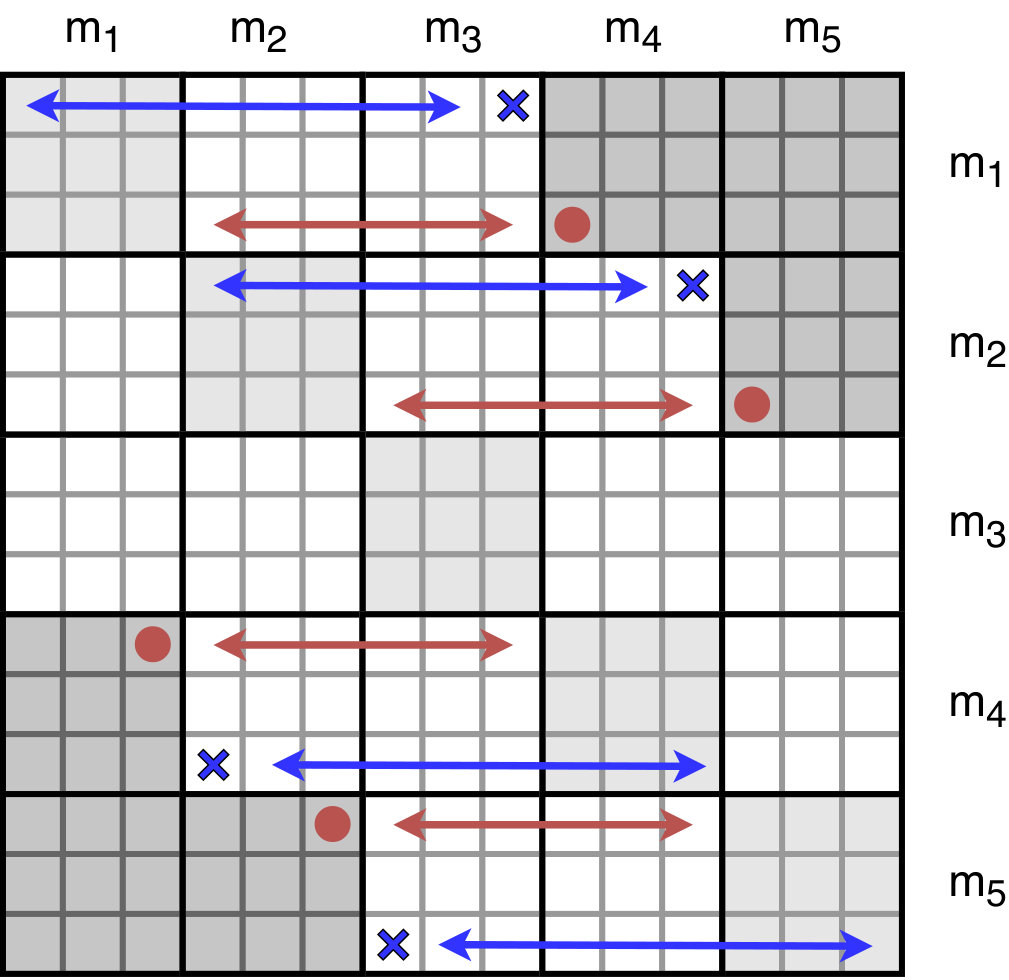 Figure 1
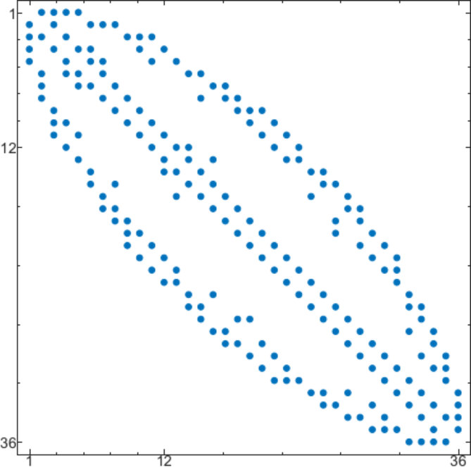 Figure 2
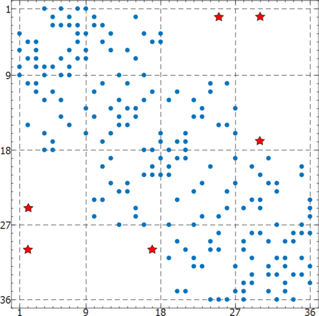 Figure 3
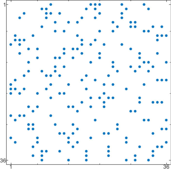 Figure 4
| \bigstrut | |||||||
| 16 | 8 | 8 | 17 | 6 | 1.23 | ||
| 15 | 9 | 9 | 16 | 5 | - | ||
| 11 | 9 | 9 | 9 | 11 | 6 | 0.68 | |
| 9 | 10 | 10 | 10 | 10 | 5 | - | |
| 6 | 9 | 9 | 9 | 9 | 7 | 6 | 0.56 |
| 4 | 10 | 10 | 10 | 10 | 5 | 4 | - |
| \bigstrut | |||||||
| 23 | 9 | 9 | 23 | 7 | 1.01 | ||
| 22 | 10 | 10 | 22 | 6 | - | ||
| 17 | 10 | 10 | 10 | 17 | 7 | 0.84 | |
| 15 | 11 | 11 | 11 | 16 | 7 | - | |
| 12 | 10 | 10 | 10 | 10 | 12 | 8 | 0.99 |
| 10 | 11 | 11 | 11 | 11 | 10 | 6 | - |
| \bigstrut | |||||||
| 31 | 9 | 9 | 32 | 9 | 1.53 | ||
| 30 | 10 | 10 | 31 | 8 | - | ||
| 25 | 10 | 10 | 10 | 26 | 10 | 1.63 | |
| 24 | 11 | 11 | 11 | 24 | 9 | - | |
| 20 | 10 | 10 | 10 | 10 | 21 | 9 | 1.91 |
| 18 | 11 | 11 | 11 | 11 | 19 | 9 | - |
| \bigstrut | |||||||
| 41 | 9 | 9 | 41 | 11 | 1.62 | ||
| 40 | 10 | 10 | 40 | 10 | - | ||
| 32 | 12 | 12 | 12 | 32 | 10 | 0.68 | |
| 30 | 13 | 13 | 13 | 31 | 9 | - | |
| 24 | 13 | 13 | 13 | 13 | 24 | 10 | 0.52 |
| 22 | 14 | 14 | 14 | 14 | 22 | 10 | - |
| \bigstrut | |||||||
| 14 | 10 | 10 | 15 | 5 | 0.87 | ||
| 13 | 11 | 11 | 14 | 3 | - | ||
| 8 | 11 | 11 | 11 | 8 | 2 | 0.18 | |
| 6 | 12 | 12 | 12 | 7 | 1 | - | |
| 2 | 11 | 11 | 11 | 11 | 3 | 3 | 0.07 |
| \bigstrut | |||||||
| 21 | 11 | 11 | 21 | 7 | 0.76 | ||
| 20 | 12 | 12 | 20 | 5 | - | ||
| 14 | 12 | 12 | 12 | 14 | 6 | 0.64 | |
| 12 | 13 | 13 | 13 | 13 | 3 | - | |
| 8 | 12 | 12 | 12 | 12 | 8 | 6 | 0.35 |
| 6 | 13 | 13 | 13 | 13 | 6 | 3 | - |
| \bigstrut | |||||||
| 28 | 12 | 12 | 29 | 10 | 0.96 | ||
| 27 | 13 | 13 | 28 | 7 | - | ||
| 21 | 13 | 13 | 13 | 21 | 8 | 1.12 | |
| 19 | 14 | 14 | 14 | 20 | 6 | - | |
| 14 | 13 | 13 | 13 | 13 | 15 | 10 | 1.34 |
| 12 | 14 | 14 | 14 | 14 | 13 | 7 | - |
| \bigstrut | |||||||
| 37 | 13 | 13 | 37 | 11 | 0.64 | ||
| 36 | 14 | 14 | 36 | 9 | - | ||
| 29 | 14 | 14 | 14 | 29 | 11 | 1.20 | |
| 27 | 15 | 15 | 15 | 28 | 9 | - | |
| 22 | 14 | 14 | 14 | 14 | 22 | 11 | 1.64 |
| 20 | 15 | 15 | 15 | 15 | 20 | 9 | - |
| \bigstrut | ||||
|---|---|---|---|---|
| 7 | 49 | 10 | 12 | 14 |
| 8 | 64 | 11 | 13 | 16 |
| 9 | 81 | 11 | 14 | 18 |
| 10 | 100 | 14 | 15 | 20 |
| Hypercube \bigstrut | |||||||||
| - | - | ||||||||
| 6 | 10 | 10 | 6 | 0 | - | ||||
| 7 | 9 | 9 | 7 | 4 | 0.99 | 10 | |||
| Hypercube \bigstrut | |||||||||
| r | |||||||||
| 15 | 17 | 17 | 15 | 10 | 1.18 | 18 | 1 | ||
| 15 | 9 | 8 | 9 | 8 | 15 | 14 | 1.18 | 18 | 2 |
| 14 | 9 | 9 | 9 | 9 | 14 | 9 | - | ||
| Hypercube \bigstrut | |||||||||
| 33 | 31 | 31 | 33 | 19 | - | ||||
| 34 | 30 | 30 | 34 | 31 | 3.11 | 31 | |||
| 16 | 32 | 32 | 32 | 16 | 18 | 0.93 | 33 | ||
| Name | bdw-dens | |||||||
|---|---|---|---|---|---|---|---|---|
| partitioning | ||||||||
| 3 | 4 | 5 | 6 | |||||
| DWT59 | 59 | 104 | 6 | 0.381 | 3 | 4 | 4 | 5 |
| DWT87 | 87 | 227 | 10 | 0.278 | 5 | 6 | 7 | 8 |
| NOS4 | 100 | 247 | 10 | 0.261 | 6 | 7 | 7 | 8 |
| ASH85 | 85 | 219 | 9 | 0.304 | 4 | 6 | 7 | 7 |
| CAN61 | 61 | 248 | 13 | 0.353 | 5 | 9 | 9 | 11 |
| CAN73 | 73 | 152 | 16 | 0.147 | 7 | 11 | 14 | 14 |
| CAN96 | 96 | 336 | 13 | 0.290 | 7 | 10 | 11 | 12 |
| GD97-b | 47 | 132 | 15 | 0.226 | 5 | 11 | 12 | 11 |
| mesh1e1 | 48 | 129 | 11 | 0.279 | 6 | 9 | 10 | 10 |
| sphere2 | 66 | 192 | 13 | 0.250 | 7 | 9 | 11 | 12 |
| dolphins | 62 | 159 | 13 | 0.222 | 7 | 9 | 11 | 11 |
| lesmis | 77 | 254 | 20 | 0.191 | 5 | 11 | 16 | 17 |
| polbooks | 105 | 441 | 20 | 0.233 | 9 | 11 | 14 | 17 |
| adjnoun | 112 | 425 | 39 | 0.119 | 23 | 32 | 31 | 32 |
| football | 115 | 613 | 37 | 0.173 | 28 | 33 | 33 | 33 |
Peer Reviews
No public reviews on file for this paper yet. If you reviewed it on a platform where reviews are public (OpenReview, ICLR, NeurIPS, ICML), you can paste yours below so the community can read it here.
Videos
No videos yet. Explain this paper in a talk, walkthrough, or lecture? Add one.
\xspaceaddexceptions
[]{}
Lower Bounds for the Bandwidth Problem
111 This project has received funding from the European Union’s Horizon 2020 research and innovation programme under the Marie Skłodowska-Curie grant agreement No 764759 and the Austrian Science Fund (FWF): P 28008-N35.
Franz Rendl
Department of Mathematics, Alpen-Adria-Universität, Klagenfurt, Austria
Renata Sotirov
Department of Econometrics and OR, Tilburg University, The Netherlands
Christian Truden
Department of Mathematics, Alpen-Adria-Universität, Klagenfurt, Austria
Abstract
The Bandwidth Problem seeks for a simultaneous permutation of the rows and columns of the adjacency matrix of a graph such that all nonzero entries are as close as possible to the main diagonal. This work focuses on investigating novel approaches to obtain lower bounds for the bandwidth problem. In particular, we use vertex partitions to bound the bandwidth of a graph. Our approach contains prior approaches for bounding the bandwidth as special cases. By varying sizes of partitions, we achieve a trade-off between quality of bounds and efficiency of computing them. To compute lower bounds, we derive a Semidefinite Programming relaxation. We evaluate the performance of our approach on several data sets, including real-world instances.
Keywords. Bandwidth Problem, Graph Partition, Semidefinite Programming.
1 Introduction
The Bandwidth Problem (BP) is the problem of labeling the vertices of a given undirected graph with distinct integers such that the maximum difference between the labels of adjacent vertices is minimal. It originated in the 1950s from sparse matrix computations, and received much attention since Harary’s [16] description of the problem and Harper’s paper [18] on the bandwidth of the -cube (see also [6, 12]). Berger-Wolf and Reingold [2] showed that the problem of designing a code to minimize distortion in multi-channel transmission can be formulated as the Bandwidth Problem for generalized Hamming graphs. The BP belongs to a class of combinatorial optimization problems known as graph layout problems. The Cyclic Bandwidth [35, 11], Cutwidth [27, 5], Antibandwidth [25] and Linear Arrangement Problem [17, 34] also belong to this class of problems. The Bandwidth Problem arises in many different engineering applications related to efficient storage and processing. It also plays a role in designing parallel computation networks, VLSI layouts, and constraint satisfaction problems, see e.g., [6, 12, 24] and the references therein.
Determining the bandwidth is NP-hard [31] and even approximating the bandwidth within a given factor is known to be NP-hard [39]. Moreover, the BP is known to be NP-hard even on trees with maximum degree three [14] and on caterpillars with hair length three [28]. On the other hand, the Bandwidth Problem has been solved for a few families of graphs having special properties. Among these are the path, the complete graph, the complete bipartite graph [7], the hypercube graph [18], the grid graph [8], the complete -level -ary tree [36], the triangular graph [22], and the triangulated triangle [20]. Blum et al. [3] and Dunagan and Vempala [13] propose an approximation algorithm for the bandwidth, where is the number of vertices.
Several lower and upper bounding approaches for the bandwidth of a graph are considered in the literature. Cuthill and McKee [9] proposed a heuristic to relabel the vertices of the graph so as to reduce the bandwidth after relabeling. It is widely used in practice, see for instance [38]. MATLAB offers the command symrcm as an implementation of this heuristic. For graphs with symmetry there exists an improved reverse Cuthill-McKee algorithm, see [40]. However, it is much more difficult to obtain lower bounds on the bandwidth. The following two approaches have been proposed in the literature.
Lower bounds based on 3-partitions
Juvan and Mohar [23] consider 3-partitions of the vertices into partition blocks of (fixed) sizes and . If all such partitions have edges joining and , then clearly the bandwidth must be bigger than . Juvan and Mohar introduce eigenvalue-based lower bounds on the bandwidth which were refined by Helmberg et al. [19] leading to the following bound based on eigenvalues of the Laplacian of the graph
[TABLE]
see also the subsequent section. The same lower bound was derived by Haemers [15] by exploiting interlacing of Laplacian eigenvalues. Povh and Rendl [32] showed that this eigenvalue bound can also be obtained by solving a Semidefinite Programming (SDP) relaxation for a special Minimum Cut (MC) problem. They further tightened the SDP relaxation and consequently obtained a stronger lower bound for the Bandwidth Problem. Rendl and Sotirov [33] showed how to further tighten the SDP relaxation from [32].
Bounds based on permutations
A labeling of the vertices of a graph corresponds to a simultaneous permutation of the rows and columns of the adjacency matrix. This may be expressed by pre- and post-multiplication with a permutation matrix, leading to quadratic assignment formulations of the bandwidth. De Klerk et al. [11] proposed two lower bounds based on SDP relaxations of the resulting Quadratic Assignment Problem (QAP). The numerical results in [11] show that both their bounds dominate the bound of Blum et al. [3], and that in most of the cases their bounds are stronger than the bound by Povh and Rendl [32].
In [40], the authors derived an SDP relaxation of the minimum cut problem by strengthening the well-known SDP relaxation for the QAP. They derive strong bounds for the bandwidth of highly symmetric graphs with up to 216 vertices by exploiting symmetry. For general graphs, their approach is rather restricted. Above mentioned bounds are either unsatisfyingly weak, or computing them is challenging already for small (general) graphs, i.e., graphs of about vertices.
Our contribution
We introduce a general -partition model to get lower bounds on the bandwidth. It contains (with ) the 3-partition model from Juvan and Mohar [23] and (with ) the permutation-based formulation of the problem, see Section 3 below. The -partition problem is still NP-complete. Therefore, we introduce tractable relaxations based on SDP. In Section 4 such a relaxation based on the “matrix-lifting” idea is introduced. It leads to an SDP in matrices of order . It is known that the feasible region of such a relaxation always has a nullspace of dimension . We identify an -dimensional part of this nullspace, which can be eliminated using a simple combinatorial argument. Finally, in Section 5, we show that the new partition model leads to improved lower bounds for the bandwidth, even in case of small values of , like . Moreover, we provide strong bounds for graphs with up to vertices in a reasonable time frame.
Notation
The space of symmetric matrices is denoted by and the space of symmetric positive semidefinite matrices by . For two matrices , , means , for all . The set of permutation matrices is denoted by . Further, for a matrix the corresponding transposed matrix is denoted by while denotes the orthogonal complement. We use to denote the identity matrix of order , and to denote the -th standard basis vector of length . Similarly, and denote the all-ones matrix and all-ones -vector, respectively.
The trace operator is denoted by trace, and denotes the trace inner product. The Hadamard product of two matrices and of the same size is denoted by and defined as for all . The diag operator maps an matrix to the -vector given by its diagonal, while the vec operator stacks the columns of a matrix in a vector. We denote by Diag the adjoint operator of diag.
2 The Bandwidth Problem
We now formally introduce the Bandwidth Problem as a Quadratic Assignment Problem with special data matrices and .
Let be an undirected simple graph with vertices and edge set . A bijection is called a labeling of the vertices of . The bandwidth of a graph with respect to the labeling is defined as follows
[TABLE]
The bandwidth of a graph is defined as the minimum of over all labelings , i.e.,
[TABLE]
Equivalently, one can consider the adjacency matrix of the graph . The bandwidth of amounts to a simultaneous permutation of the rows and columns of the adjacency matrix such that the largest distance of a nonzero entry from the main diagonal is as small as possible. The bandwidth of an adjacency matrix is defined as:
[TABLE]
Therefore, from now on we assume that a graph is given through its adjacency matrix . Since in terms of matrices the BP seeks for a simultaneous permutation of the rows and columns of such that all nonzero entries are as close as possible to the main diagonal, a “natural” problem formulation is as follows.
Let be an integer such that , and be the symmetric matrix of order defined as follows
[TABLE]
Then, the following holds:
[TABLE]
The minimization problem has the form of a QAP, which might be even harder to solve than actually computing . The idea of formulating the Bandwidth Problem as a QAP was suggested by Helmberg et al. [19]. De Klerk et al. [11] considered two SDP-based bounds for the Bandwidth Problem that are obtained from the SDP relaxations for the QAP introduced in [42] and [10]. The results show that it is hard to obtain bounds for graphs with vertices, even though the symmetry in the graphs under consideration was exploited.
Since it is very difficult to solve QAPs in practice for sizes larger than vertices other approaches are needed for deriving bounds for the bandwidth of graphs.
3 Partition Approach
We show how to use vertex partitions in order to obtain lower bounds for the bandwidth of a graph. For let be given with (), . We consider partitions of the vertex set into subsets such that . These are in one-to-one correspondence with partition matrices:
[TABLE]
where for the partition we set whenever , . Since any vertex is assigned to precisely one of the blocks we can define the map given by
[TABLE]
which identifies the partition block containing vertex . Thus, given the partition matrix we get for all . For let be the 0–1 matrix of order with
[TABLE]
Suppose that , i.e., . Then for the following holds:
[TABLE]
Therefore we get
[TABLE]
Hence, this term counts the number of edges with endpoints in partition blocks of distance greater than under the map .
Basic Partition
It will be convenient to introduce the special partition matrix corresponding to the basic partition which assigns the first vertices to the next vertices to and so on. Thus, the matrix is characterized by columns of consecutive blocks of ones of appropriate lengths. Therefore the matrix
[TABLE]
is a block matrix with blocks of sizes . The nonzero blocks of this matrix correspond to all-ones matrices of size whenever the entry , see also Figure 1 below. Thus, for a given adjacency matrix the term counts the number of edges joining vertices in partition blocks of distance greater than .
General Partition
In general, any partition matrix can be obtained from the basic partition matrix by row-permutations that are defined by a permutation matrix . Thus
[TABLE]
where is the basic partition matrix. The following transformation is obtained by replacing by :
[TABLE]
This shows that the permutation can be applied either to the adjacency matrix or to the matrix .
The following example serves as an illustration of this property.
Example 1**.**
We consider a matrix and the partitioning . Moreover, we choose . If , then there must be an edge with endpoints in blocks of distance larger than . Such edges could either join vertices in and , or in and , or in and , which require to “jump” over or at least. We illustrate this in Figure 1.
The following theorem forms the basis for our lower bounds on the bandwidth.
Theorem 1**.**
Let be an adjacency matrix, and let and be given with . Let . If
[TABLE]
[TABLE]
Proof.
If then some nonzero entry of is multiplied with a nonzero entry of . The nonzeros of this matrix closest to the main diagonal are in the positions
[TABLE]
As an illustration, these positions are marked with bullets in Figure 1 below. The distances of these positions to the main diagonal are given by
[TABLE]
Therefore must be larger than the smallest of these numbers. ∎
In case that the above minimum is zero, we have to consider the zeros of with largest possible distance to the main diagonal. These are marked with crosses in Figure 1.
Theorem 2**.**
Let be an adjacency matrix, and let and be given with . Let . If
[TABLE]
[TABLE]
The proof is similar to Theorem 1 and is therefore omitted. In Figure 1, we illustrate the lower and upper bounds given by Theorems 1 and 2, respectively.
The following Minimal Partition Problem ():
[TABLE]
serves as the basis to derive lower bounds on the bandwidth of . From a practical point of view, we are interested in selections of where the minimum in Theorem 1 is attained in each term. Some particular cases are summarized in the following corollaries.
Corollary 3**.**
Let be an adjacency matrix of , and let and be given with . Let . Further, suppose that .
If there exists such that , then .
Corollary 4**.**
Let be an adjacency matrix of , and let and be given with . Further, suppose .
If there exists such that , then
By cyclically repeating the sizes, we can insure that the minimum in Theorem 1 is attained in each term simultaneously as above also for values .
3.1 Relation to Prior Work
We present below two important special cases of our new modelling approach and their relation to prior work.
The case
Given the only allowable choice for is and therefore the only nonzero elements in are . Hence for Theorem 1 states that if there exists such that , then . This observation is used in [19] to derive lower bounds on , and is further refined in [32, 40].
The case
Another notable case occurs for , which implies that . Hence, for any it follows from Theorem 1 that , if there exists a partition matrix such that . However, in this case the basic partition matrix becomes the identity matrix of rank , i.e., . Thus, becomes a permutation matrix and we recover the statement
[TABLE]
from (1). This approach is used e.g., in [11] to derive lower bounds on .
In Summary, we have shown that once the problem has a positive value for given and , we get a nontrivial lower bound on the bandwidth from Theorem 1. The problem is itself NP-complete, so our strategy is to consider tractable lower bounds for the problem. If some lower bound turns out to be positive for given and , then clearly has a positive value, and our bounding argument can be applied. In the following section we consider relaxations of , based on semidefinite optimization.
4 SDP models
In this section, we derive several Semidefinite Programming relaxations for the Minimal Partition Problem. Our first two SDP relaxations are obtained by matrix lifting and therefore have matrix variables of order , while the third relaxation has matrix variables of order .
4.1 SDP model in
In this section, we derive an SDP relaxation whose matrix variable is of order .
Let be a partition matrix, see (2). Let be the columns of , i.e., , and . Now, the constraint may be weakened to which is well-known to be equivalent to the following convex constraint
[TABLE]
Further, we use the following block notation for :
[TABLE]
where corresponds to , and to .
For any , we have and thus . For all we have:
[TABLE]
Similarly, we have
[TABLE]
From orthogonality of vectors , , it follows \textbf{diag}\big{(}X_{ij}\big{)}=0.
Let us describe the matrix (3) as the sum of symmetric matrices having only two non-zero entries, i.e., Hence, we derive
[TABLE]
Therefore, we can rewrite the Minimal Partition Problem, see (4), as:
[TABLE]
Finally, we collect all above mentioned constraints and propose the following model for the Minimal Partition Problem based on the matrix lifting approach.
[TABLE]
Here . The feasible region of the above SDP relaxation equals the feasible region of the SDP relaxation for the graph partition problem derived by Wolkowicz and Zhao [41]. In order to further improve the relaxation, one can add nonnegativity constraints.
Below, we analyze the feasible region of the model (5).
Lemma 5**.**
Let satisfy (5b), (5c), (5d), (5e), and (5g). Then
[TABLE]
spans the nullspace of .
For a proof we refer the reader to [33, Lemma 10 and Section 5.2] as well as to [41]. We observe in particular that this result holds independent of (5f).
Note that the vectors from Lemma 5 correspond to a matrix. As the sum of the first columns is equal to the sum of the last columns, the nullspace of has dimension .
Lemma 6**.**
Let satisfy (5b), (5c), (5d), (5e), and (5g). Then
[TABLE]
Again, we refer the reader to [33, Section 5.2], and [41] for a formal proof. As a consequence of the previous lemma, the block is determined by , , (), and . Hence, matrix can be reduced by one block of rows and their corresponding columns without loss of information. This leads us to the reduced SDP model presented in the following section.
One can also derive the Slater feasible version of the SDP relaxation (5) by exploiting a basis of the orthogonal complement to the nullspace of given in Lemma 5. For details see e.g., [42, 33]. The Slater feasible version may be efficiently solved by using the Alternating Direction Method of Multipliers (ADMM) as described in [30]. The ADMM is a first-order method for convex problems that decomposes an optimization problem into subproblems that may be easier to solve.
4.2 Reduced SDP Model in
In this section, we provide an SDP relaxation that is equivalent to the one from the previous subsection, but contains less variables. In particular, based on Lemma 6, we propose the following SDP relaxation for the Minimal Partition Problem.
[TABLE]
Here . Note that the nullspace of the reduced matrix has rank . We show below that the SDP relaxation (6) is equivalent to (5).
The number of equations in this SDP is still , but we saved about equations as compared to the original model.
Additional sign constraints
[TABLE]
insure that the lower bound from this model is always nonnegative.
Lemma 7**.**
From (6b) – (6g) follow (5b) – (5g).
Proof.
Step 1: From Lemma 6 directly follows that, given , the “missing” entries of can be expressed by:
[TABLE]
Nonnegativity of follows from (6c) and (6g).
Step 2:
Constraint (5g)
From [33, Section 5], we know that under (6b) – (6g) it holds that
[TABLE]
where
[TABLE]
Hence, it holds (5g).
Constraint (5b)
In addition to (6b), must hold. In particular, from Step 1 it follows
[TABLE]
Constraint (5c)
In addition to (6c), , must hold. Again, by using Step 1 we have:
[TABLE]
Constraint (5d)
From (6b) and Step 1 we have (5b).
Thus, from it follows \textbf{trace}\big{(}X_{k}\big{)}=m_{k}.
Constraint (5e)
From and , we have
[TABLE]
Constraint (5f)
In addition to (6f), , must hold.
[TABLE]
∎* *
Note that the inverse to the one in the lemma follows directly. To make the SDP relaxation (6) with additional nonnegativity constraints equivalent to SDP relaxation (5) with additional nonnegativity constraints, we need to add nonnegativity constraints to the “missing” blocks in (6). In particular, we have the following proposition.
Proposition 8**.**
The SDP relaxation (5) with additional constraints is equivalent to the SDP relaxation (6) with additional constraints and
[TABLE]
where .
In Section 5, we demonstrate the strength of our SDP relaxation.
5 Computational Experiments
5.1 Solving the SDP relaxation
The partition-based lower bounds for the bandwidth problem lead to semidefinite programs with one matrix of dimension , see (6). The resulting relaxations can be solved using standard SDP packages such as SDPT3 only for limited values of and . We also consider nonnegativity constraints which add another potentially violated sign constraints to our relaxation. Interior-point based methods for such a scenario turn out to be too slow. Hence, we propose to use the ADMM method, which works well for SDPs with simple sign constraints. To use the ADMM, we use the Slater feasible version of the SDP relaxation (5) as described in the previous section. The resulting SDP relaxation has a matrix variable of order , see e.g., [41]. Then, we proceed in the same manner as described in [30, 21].
5.2 Strength of the partition bounds
As a first experiment we investigate the quality of the SDP relaxations (5) and (6) to assess
[TABLE]
for given and . We recall that minPart() denotes the number of edges in the minimal partition specified by and , see (4). We are primarily interested in parameter settings for and where minPart but small. For such values of and it is a nontrivial task to prove positive lower bounds for minPart using our SDP models.
5.2.1 Test problems
We investigate the practical performance of our lower bounds on the following classes of graphs.
Torus graphs
For given integer the torus graph has vertices which we label by for . We introduce “vertical” edges of the form for and . Altogether there are such edges. In a similar way we add “horizontal” edges of the form for together with . This graph therefore has vertices and edges. These graphs are interesting for the following reason. They are extremely sparse ( vertices and edges), but their bandwidth is quite large. Namely, it is known that , see e.g., [1, 26].
Torus graphs plus Hamiltonian path
Here we start out with the torus graph , choose a labeling of its vertices yielding a bandwidth of size , and add the Hamiltonian path from the first to the last vertex in this labeling. The resulting graph is denoted by . It is still sparse having roughly edges and bandwidth again at most .
Hypercubes
The Hamming graph is the Cartesian product of copies of the complete graph . The Hamming graph is also known as the hypercube (graph) . Thus, the hypercube graph has vertices. The bandwidth of the hypercube graph was determined by Harper [18] and is given by the following expression:
[TABLE]
We use the hypercube graphs to test the quality of our partition bounds.
5.2.2 Computations
Torus graphs
In the tables to follow we always provide the following information. The first block of data contains the vector of cardinalities for the partition blocks. We consider partitions into blocks. We set and ask that
The sizes and are chosen such that and Next we provide upper and lower bounds for the Minimal Partition Problem. The upper bound (ub) is obtained by running a standard Simulated Annealing heuristic [4] to find a good partition. The lower bound (lb) is obtained from the SDP relaxation (5) with all nonnegativity constraints included. Our main interest lies in values of , where the obtained lower bound is nontrivial, i.e., . We give an illustration of the obtained solutions in Figure 2.
First, we consider Table 1, which contains computational results for the Torus graph . Initially, we consider 4 blocks with leading to a lower bound . Hence, Corollary 3 allows us to conclude that . We next try where we only obtain the trivial lower bound of [math]. Therefore, we get no further restriction on from 4-partitions. The 5-partition with however yields a positive lower bound and therefore . Also, 6-partitions, given in the last block of the Table 1, do not lead to a further tightening of .
The results for the Torus graphs , and are summarized in Table 2. We proceed as before and consider partitions with . We can prove a lower bound of for and . It turns out that proving positive lower bounds for our partition problems gets increasingly difficult as either or increases. For , the use of a 6-partition allows us to prove a lower bound of .
As a second experiment, we consider the graphs consisting of the union of the Torus graph and a Hamiltonian path such that is insured. The results are summarized in Table 3. Compared to the Torus graphs we get slightly stronger lower bounds even though these graphs are still quite sparse, with . Again, we see increasing gaps between lower and upper bounds as the number of nodes of the graph increases.
We summarize the bandwidth information for all variations of the Torus graphs in Table 4. Our partitioning approach provides nontrivial lower bounds on all instances.
Now, let us provide some information on computation time. To compute 4-partitions for graphs with 49 vertices we need about seconds, for 5-partitions about seconds, and for 6-partitions about seconds. On the other hand, to compute a 4-partition (6-partition) on a graph with 100 vertices, our ADMM code needs about seconds ( seconds). Clearly, computation times increase with respect to increasing partition sizes and number of vertices of the graphs. However, we obtain bounds in reasonable time for all tested graphs. All experiments were performed on a Windows 7 64-bit machine equipped with an Intel Core i5-5300U (22300 MHz) and 12 GB RAM using MATLAB 2016b.
Hypercubes
Results for the hypercubes , , and are summarized in Table 5. The table reads similar to the previous tables. To show a lower bound of 10 for , our ADMM needs only 4 seconds. For comparison purposes we computed a lower bound for and the case . Thus, we solved the QAP relaxation for that instance and obtained as the lower bound of the BP.
For the hypercube the 4-partition with and yields a positive lower bound, and therefore . We also compute the 6-partition with and , and obtain a positive lower bound, which leads again to the conclusion that . Finally, we prove a lower bound of 33 for the hypercube .
5.3 Bandwidth of Matrices from Applications
In this section, we evaluate the performance of our approach on matrices that are given by real-world applications. We collected symmetric matrices, having to vertices. These are taken from the HB, Pothen, and Pajek groups of the SuiteSparse Matrix Collection [37]. We also selected matrices from the Newman collection available on the NIST Matrix Market [29].
Considering the Bandwidth Problem, only the structural properties of the matrices are of interest. Therefore, for a matrix , we set . Moreover, we set all nonzero entries equal to one.
In our computational evaluation, we select the partitioning such that , , and where . We set , except when applying the 6-partition to adjnoun and football where we had to set . In the later case, we apply Corollary 4.
We summarize the results in Table 6. We provide the number of nodes (column labeled ) and the number of edges (column labeled ). The column labeled provides an upper bound on the bandwidth which we found by running a Simulated Annealing heuristic. We did not find any bandwidth information on these data in the literature. We also determined the density relative to the bandwidth, i.e., proportion of edges within the bandwidth, in the column labeled (bdw-dens). Finally, and most interestingly, we provide lower bounds based on -partitions for . The results in the column for reflect the previous state-of-the-art using 3-partitions. The remaining columns show the improvement of the lower bound using partitions into blocks. The lower bound is substantially improved in all cases. These results clearly indicate that our general partition approach yields a significant improvement over the 3-partition bounds from [23, 19, 32, 33].
5.4 Discussion
Based on our computational experiments we reach the following conclusions.
- •
The partitioning approach leads to acceptable lower bounds for the Bandwidth Problem. Our results indicate that the bounds get weaker as the number of nodes increases. This should come as no surprise in view of the hardness results known for the Bandwidth Problem.
- •
Our approach offers some flexibility in choosing the number of partition blocks to estimate the bandwidth. A larger would result in tighter bounds at higher computational cost.
- •
Further tightening of the semidefinite models is possible by adding additional constraints, e.g., triangle inequalities. This results in SDPs which require a refined computational setup.
- •
We could prove significantly better lower bounds for the Bandwidth Problem compared to the previous state-of-the-art of using 3-partitions.
6 Summary and Conclusion
We have shown that the partition approach provides a versatile tool to obtain lower bounds for the bandwidth of a graph. The choice of the model parameters , , and are highly problem dependent. However, our experiments indicate that even with a small number of partition blocks () we are able to derive nontrivial lower bounds on the bandwidth, even for very sparse graphs. Further research is necessary to explore this approach for larger graphs.
The reference list from the paper itself. Each links out to its DOI / PubMed record.
- 1Balogh et al. [2006] József Balogh, Dhruv Mubayi, and András Pluhár. On the edge-bandwidth of graph products. Theoretical Computer Science , 359(1):43–57, 2006. ISSN 0304-3975. doi: 10.1016/j.tcs.2006.01.046 . · doi ↗
- 2Berger-Wolf and Reingold [2002] Tanya Y. Berger-Wolf and Edward M. Reingold. Index assignment for multichannel communication under failure. IEEE Transactions on Information Theory , 48(10):2656–2668, Oct 2002. ISSN 0018-9448. doi: 10.1109/TIT.2002.802643 . · doi ↗
- 3Blum et al. [2000] Avrim Blum, Goran Konjevod, R. Ravi, and Santosh Vempala. Semi-definite relaxations for minimum bandwidth and other vertex-ordering problems. Theoretical Computer Science , 235(1):25–42, 2000. ISSN 0304-3975. doi: 10.1016/S 0304-3975(99)00181-4 . · doi ↗
- 4Burkard and Rendl [1984] Rainer E. Burkard and Franz Rendl. A thermodynamically motivated simulation procedure for combinatorial optimization problems. European Journal of Operational Research , 17(2):169–174, 1984. ISSN 0377-2217. doi: 10.1016/0377-2217(84)90231-5 . · doi ↗
- 5Cavero et al. [2021] Sergio Cavero, Eduardo G. Pardo, Manuel Laguna, and Abraham Duarte. Multistart search for the cyclic cutwidth minimization problem. Computers & Operations Research , 126:105–116, 2021. ISSN 0305-0548. doi: doi.org/10.1016/j.cor.2020.105116 . · doi ↗
- 6[6] P. Z. Chinn, J. Chvátalová, A. K. Dewdney, and N. E. Gibbs. The bandwidth problem for graphs and matrices—a survey. Journal of Graph Theory , 6(3):223–254. doi: 10.1002/jgt.3190060302 . · doi ↗
- 7Chvátal [1970] Václav Chvátal. A remark on a problem of Harary. Czechoslovak Mathematical Journal , 20(1):109–111, 1970. URL http://eudml.org/doc/12520 .
- 8Chvátalová [1975] Jarmila Chvátalová. Optimal labelling of a product of two paths. Discrete Mathematics , 11(3):249–253, 1975. ISSN 0012-365X. doi: 10.1016/0012-365X(75)90039-4 . · doi ↗