Duality in a hyperbolic interaction model integrable even in a strong confinement: Multi-soliton solutions and field theory
Aritra Kumar Gon, Manas Kulkarni

TL;DR
This paper introduces the Hyperbolic Calogero model, a classically integrable one-dimensional system with confining potentials, and explores its multi-soliton solutions, dynamics, and field theory description through analytical and numerical methods.
Contribution
It presents the first formulation of an integrable hyperbolic interaction model with confinement, along with multi-soliton solutions and a field theory framework.
Findings
Multi-soliton solutions are analytically derived.
Numerical simulations demonstrate soliton collision dynamics.
Analytic expressions for the time period of dual variables are obtained.
Abstract
Models that remain integrable even in confining potentials are extremely rare and almost non-existent. Here, we consider a one-dimensional hyperbolic interaction model, which we call as the Hyperbolic Calogero (HC) model. This is classically integrable even in confining potentials (which have box-like shapes). We present a first-order formulation of the HC model in an external confining potential. Using the rich property of duality, we find multi-soliton solutions of this confined integrable model. Absence of solitons correspond to the equilibrium solution of the model. We demonstrate the dynamics of multi-soliton solutions via brute-force numerical simulations. We studied the physics of soliton collisions and quenches using numerical simulations. We have examined the motion of dual complex variables and found an analytic expression for the time period in a certain limit. We give the…
Click any figure to enlarge with its caption.
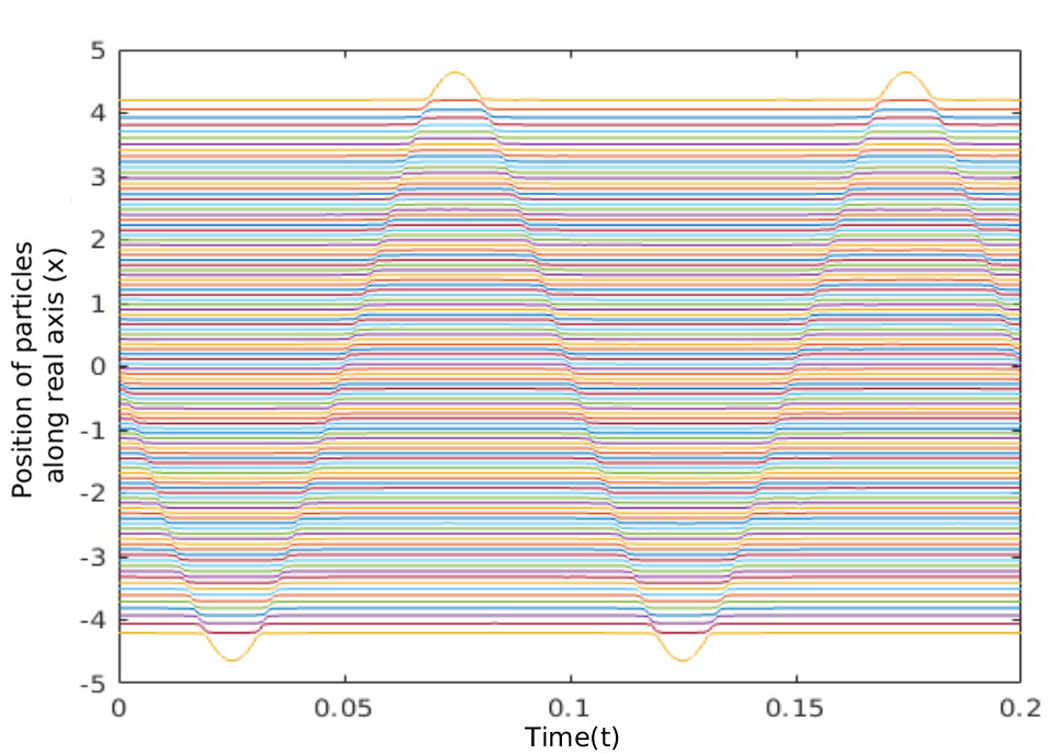 Figure 1
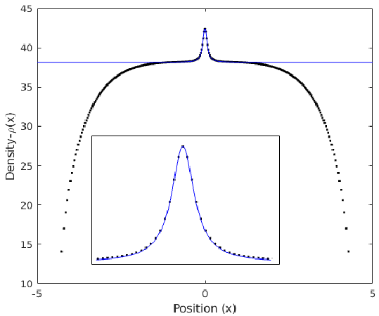 Figure 2
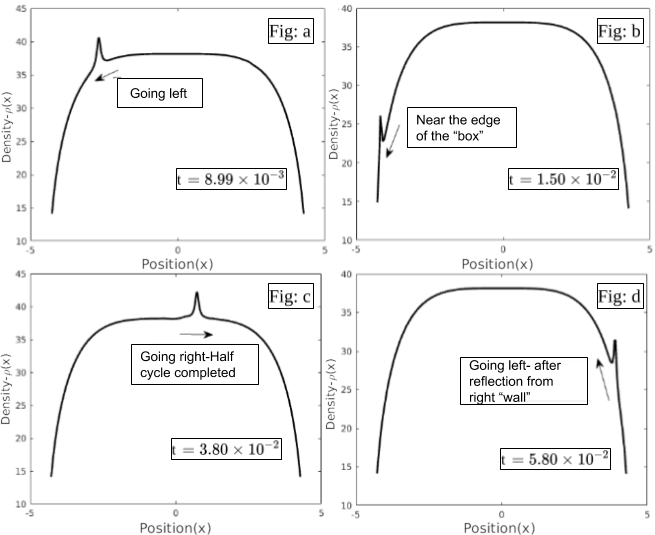 Figure 3
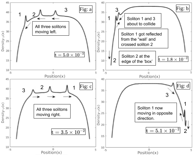 Figure 4
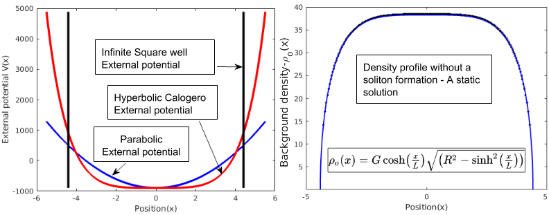 Figure 5
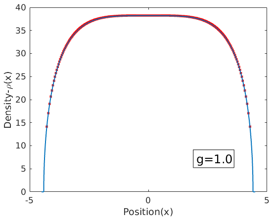 Figure 6
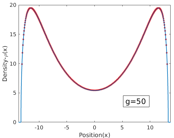 Figure 7
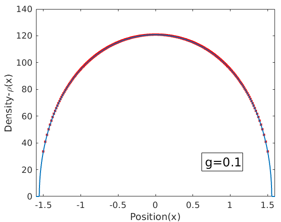 Figure 8
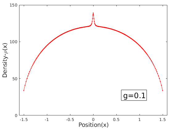 Figure 9
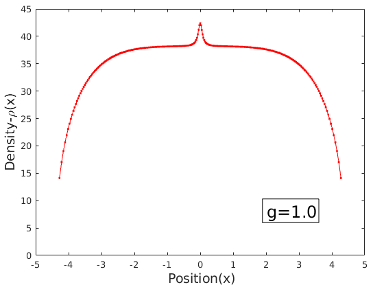 Figure 10
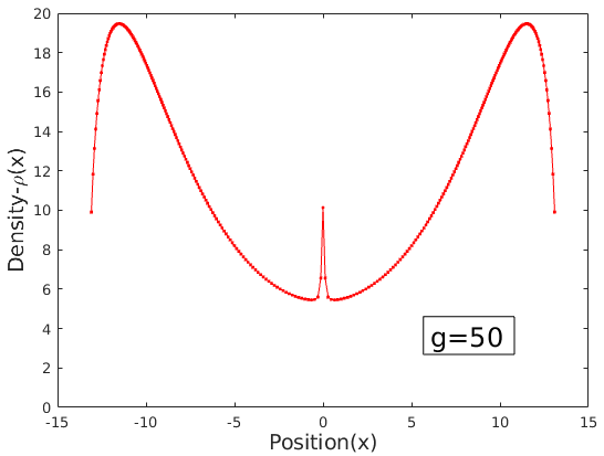 Figure 11
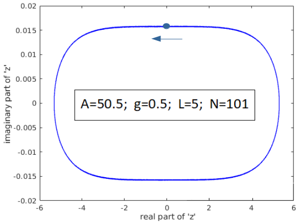 Figure 12
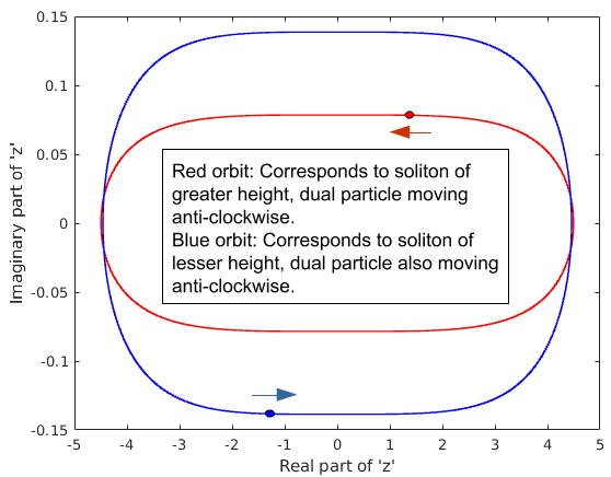 Figure 13
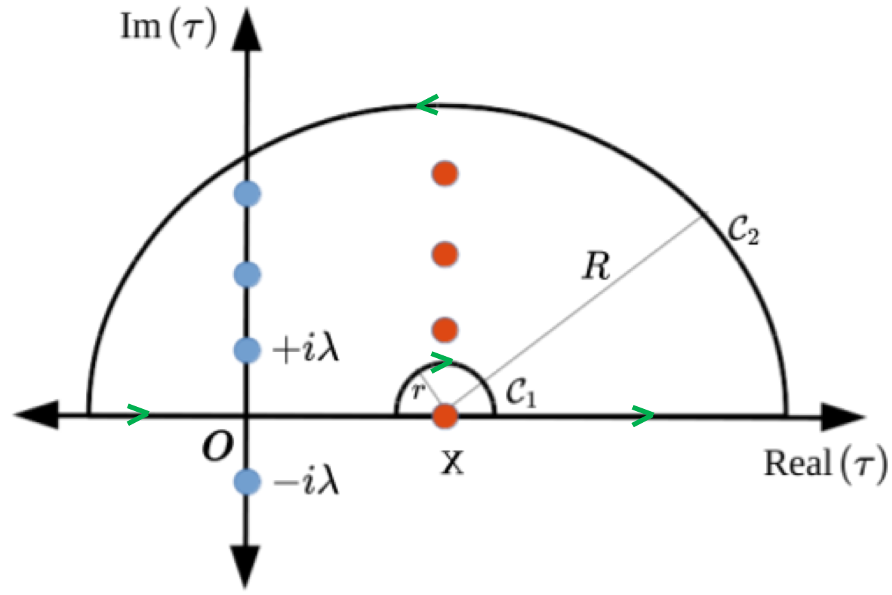 Figure 14
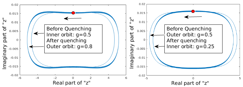 Figure 15
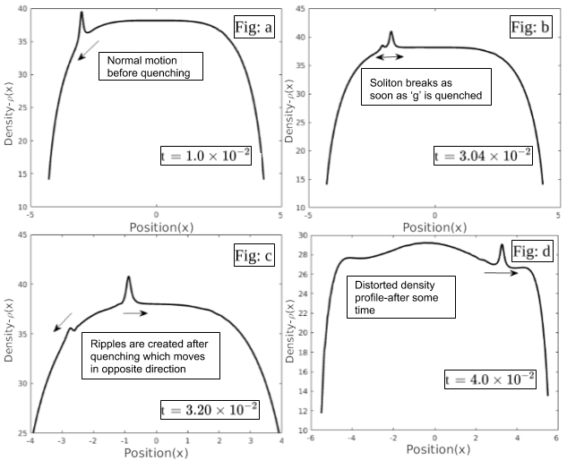 Figure 16
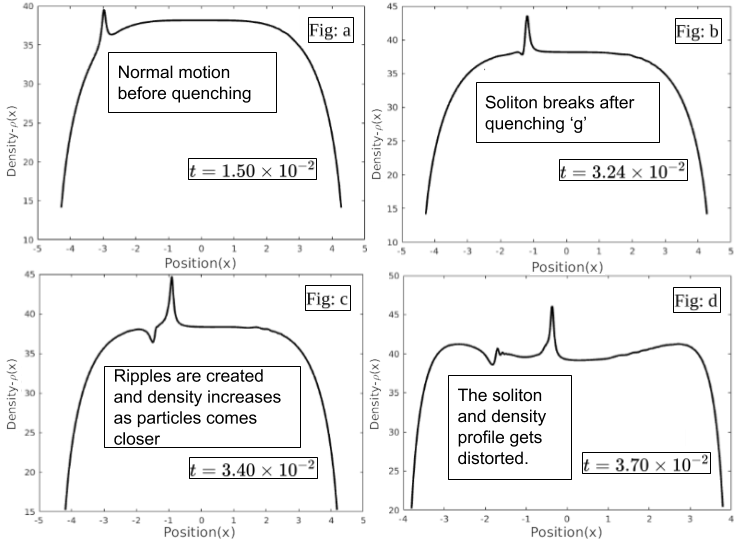 Figure 17
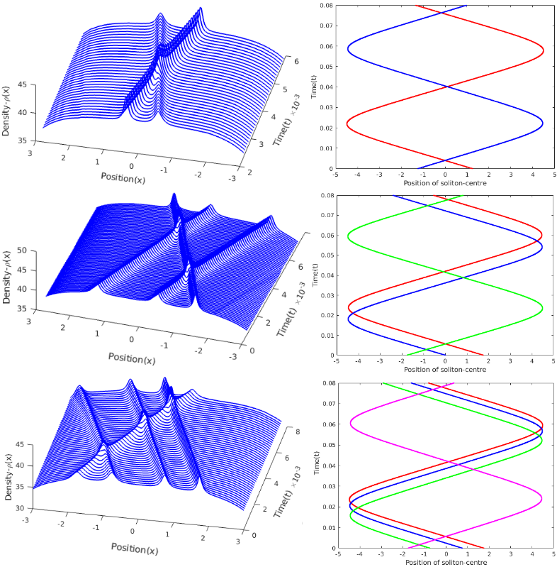 Figure 18
Peer Reviews
No public reviews on file for this paper yet. If you reviewed it on a platform where reviews are public (OpenReview, ICLR, NeurIPS, ICML), you can paste yours below so the community can read it here.
Videos
No videos yet. Explain this paper in a talk, walkthrough, or lecture? Add one.
Duality in a hyperbolic interaction model integrable even in a strong confinement: Multi-soliton solutions and field theory
Aritra Kumar Gon
Indian Institute of Technology Madras, Chennai-600036, India
International Centre for Theoretical Sciences, Tata Institute of Fundamental Research, Bangalore - 560089, India
Manas Kulkarni
International Centre for Theoretical Sciences, Tata Institute of Fundamental Research, Bangalore - 560089, India
Abstract
Models that remain integrable even in confining potentials are extremely rare and almost non-existent. Here, we consider a one-dimensional hyperbolic interaction model, which we call as the Hyperbolic Calogero (HC) model. This is classically integrable even in confining potentials (which have box-like shapes). We present a first-order formulation of the HC model in an external confining potential. Using the rich property of duality, we find multi-soliton solutions of this confined integrable model. Absence of solitons correspond to the equilibrium solution of the model. We demonstrate the dynamics of multi-soliton solutions via brute-force numerical simulations. We studied the physics of soliton collisions and quenches using numerical simulations. We have examined the motion of dual complex variables and found an analytic expression for the time period in a certain limit. We give the field theory description of this model and find the background solution (absence of solitons) analytically in the large-N limit. Analytical expressions of soliton solutions have been obtained in the absence of external confining potential. Our work is of importance to understand the general features of trapped interacting particles that remain classically integrable and can be of relevance to the collective behaviour of trapped cold atomic gases as well.
Contents
-
2 Dual Hyperbolic Calogero system and formation of the Hamiltonian
-
2.3 Relationship of background solutions with generalized Log gas
-
2.5 Multi-soliton evolutions (two ,three and four soliton solutions)
-
3.1 Single Dual variable corresponding to one soliton solution
-
3.2 Two Dual variables corresponding to two soliton solution
-
4.3 Analytic form of the density field and soliton solutions in Field Theory
1 Introduction
The rational Calogero model (with and without an external Harmonic trap) and its various generalizations is one of the most well studied integrable system in physics and mathematics [1, 2, 3, 4, 5, 6, 7]. In its traditional form, it describes identical non-relativistic particles in one dimension, interacting through two-body inverse-square potentials in the presence of an external harmonic potential [4, 8, 9]. This model and its various extensions appear in many branches of physics and mathematics and has connections and relevance to fractional statistics, fluid mechanics, spin chains, gauge theories, matrix models to name a few [10, 6, 11, 12, 13, 14, 15, 16, 17, 18]. As a result, it has been studied extensively [19, 20, 10, 21]. The rational Calogero-Moser model is a model with power-law interaction where every particle is coupled to every other particle. This is therefore considered as a relatively long-ranged model although, in 1D, it might have few properties similar to that of relatively short-ranged models [22]. It was also shown that models with inverse square interactions in 1D, for some physical quantities, have similarity with short-ranged models [23].
Given that, in most physical realizations, one has confined particles interacting with each other over some length scales, it would be of importance to study systems that remain integrable [24, 21] even in confined potentials. For e.g., a recent breakthrough in cold atomic systems has been the realization of an almost uniform gas of atoms confined in a box-like potential [25]. One of the main challenges is to find integrable models that continue to remain integrable even when they are confined in external potentials. Hence, we are looking for integrable systems with two properties: (i) Inter-particle interactions where every particle interacts with every other particle over some length-scale and (ii) Strong confinement after some legnth scale. Therefore, we study the model described below which has inter-particle interactions over some length scale, strong external confinement and the rich property of classical integrability. In addition to these properties, the model we consider has the rich property of duality and a field theory formulation.
In this paper, we investigate the behaviour of a classical system in a confining potential, interacting through an inverse square sine-hyperbolic potential. This can be viewed as a generalization of the rational Calogero-Moser model which is now periodic on the imaginary line. This is called the Hyperbolic Calogero (HC) Model.
The general form of Hamiltonian for the HC model reads,
[TABLE]
where
[TABLE]
where are the coordinates of the particles, are their canonical momenta, is a length scale associated with the model, is the coupling constant and is the number of particles. We take the mass of the particles to be unity. The above model is classically integrable [26]. Apart from the interaction between particles, another basic difference between rational and hyperbolic model is in the structure of the external potential. In the hyperbolic case, the external potential is essentially flat within a certain region from the origin and rises steeply after that thus acting like a confinement for the particles moving in it. The size of the system turns out to be L_{c}\sim L\sinh^{-1}\Big{(}\sqrt{\frac{gN}{A}}\Big{)} where is the strength of the external confining potential (to be discussed later). Particles are confined within this length. We find that the length of the system essentially scales logarithmically (hence, very slowly) with number of particles which is very different from the rational model where particles spread out as their number increases (length in rational case scales as ). This creates a major difference in the particle density profile.
In Section 2, we formulate the HC Hamiltonian with an external potential from a first order equation involving dual variables. We formulate the initial position and velocity distributions of particles for obtaining soliton solutions. This means finding a special set of initial conditions where such that when the particles move under the influence of the Hamiltonian, the density profile of the particles is a robust moving soliton. We find multi-solitons in this integrable system. This is done by solving the damping equation that we explain later. Then, we studied the dynamics of the particles for these special set of initial conditions by solving differential equations numerically. We examined the integrals of motion which provides information about the integrability of the system. We also checked the effects of two, three and four soliton collisions. We examined the effects of the various parameters on the background density (density without formation of any soliton). We have also checked the effects of quenching the parameters on the soliton motion.
In Section 3, we formulate the equations of motion for the dual variables and analyze their trajectories in the complex plane. We also check the integrals of motion. We have also examined the motion of the dual variable after quenching. We find an analytic form for the time period of oscillation of the soliton by computing periodicity of motion of the dual variables in the complex plane.
In Section 4, we derive and study the field theory formulation of this model under the continuum limit and present the corresponding soliton solutions in terms of meromorphic fields. For this discussion, the effects of the external potential are neglected as the effective length of the box was taken to be infinity. Here the particles are essentially replaced by a density field. The integrability and other rich properties of the underlying particle systems suggest that the corresponding fluid mechanical equations are also integrable and point to the existence of soliton solutions for the HC field theory (without external potential). We find out an analytic form to represent the equilibrium density distribution for the background density profile as well as for soliton solutions. We find that the equilibrium density, i.e., the background density (absence of solitons) is similar to a hyperbolic version of the trigonometric equations that appear in the context of large-N gauge theories [27, 28]. We also provide an analytic expression for soliton velocity and expressed its connection with the motion of the dual variable in the complex plane
Finally, in Section 5, we state our conclusions and provide directions of our future investigation.
2 Dual Hyperbolic Calogero system and formation of the Hamiltonian
In this section, we aim to formulate the first-order dual equations of motion for the dynamical system of particles of the confined HC model.
To start with, we consider a system of particles with coordinates , , and dual-particles with coordinates , , moving in the complex plane obeying the first-order equations of motion [8],
[TABLE]
[TABLE]
These are a set of two first order coupled differential equations describing the motion of values of and values of . The dynamics are fully described by the initial values of these + variables. One can show that if the initial values of are chosen to be real, they remain so for all future times. Using this formalism we can map the motion of particles moving in real axis to motion of dual variables moving in the complex plane. The number of dual variables are not related to the numbers of particles in the real axis, i.e. this formalism is valid even for . Remarkably the second order equations completely decouple from each other. They are of the following form,
[TABLE]
[TABLE]
Once the initial condition of positions and conjugate momenta for the particles (on the real line) are obtained using first order Eq. 3 we can study the dynamics of those particles from Eq. 5 without requiring further information about the dual variables.
The Hamiltonian corresponding to Eq. 5 is
[TABLE]
2.1 Multi-Soliton Solutions
Solitons are excitations (solitary pulse like structures) that are formed due to the collective motion of the particles. These solitons do not disperse or break down as the particles move with time. The resulting density profile (collective behaviour) is a robust excitation which does not break or disperse. Soliton solutions belong to a very special set of initial conditions in the space of initial conditions where the motion of all the particles shows a coherent behaviour. This occurs due to the delicate interplay between non-linearity, non-locality and dispersive effects. This is very sensitive to system parameters. We will further analyse its structure and behaviour in later sections.
We will now present the way by which the initial conditions for soliton solutions can be obtained in general. Note that finding soliton solutions means restricting the space of initial conditions of values of and . By equating the imaginary part of Eq. 3, we get the following equation,
[TABLE]
Equating the real part of Eq. 3, we get the conjugate momenta (),
[TABLE]
The fixed points of these set of equations in Eq. 8 give the equilibrium position of particles for obtaining soliton solution. Essentially, at that point for all . We can equivalently write Eq. 8 as,
[TABLE]
where,
[TABLE]
Therefore, we can form a damping equation [29] for a chosen set of values,
[TABLE]
where can be considered as some damping coefficient. This is actually the numerical way we employ for solving Eq. 8 for obtaining solutions corresponding to a local minimum. The damping equation in principle slides the particles towards the minimum of the above potential. The damping acts like a viscous force which slides the particles towards equilibrium position. This will finally give us the special set of and the special set is obtained from Eq. 9.
2.2 Background
The background constitutes the position of particles which corresponds to (no solitonic excitations). It gives us a static solution. From Eq. 9, it is clear that when there is no dual variable, we have values of to be equal to [math]. Hence, this is called the static solution. No soliton formation occurs. The particles just sit in their equilibrium position. For this situation, Eq. 8 becomes,
[TABLE]
Solving the corresponding damping equation, we get the positions of particles. We then plot the density of the particles as a function of position (see Fig. 1). Note that, just for plotting purpose in Fig. 1, the density is defined as the inter-particle distance and the position index is taken as the mean position between the corresponding two particles. This should not be confused with the classical density field that we introduce later in the field theory section (Sec. 4).
2.3 Relationship of background solutions with generalized Log gas
It is interesting to note that the equilibrium solutions of the classical HC model (Eq. 7 with ) which is given by Eq. 13 is also the minimum energy configuration of a generalized version of Log gas given by,
[TABLE]
Although, there has been a great deal of work on connections between traditional Log gas and Random Matrix Theory [30, 31, 32, 33] and their relation to Calogero-Moser systems [9], to the best of our knowledge, little is understood about the relationship between classical HC model, the generalized version of Log gas and Random Matrix Theory. It is to be noted that trigonometric version of the above generalized Log gas (Eq. 14) effectively appear in the context of large-N gauge theories [27, 28].
We get a plateau like graph where the density is essentially constant throughout the characteristic length of the box and falls sharply after that. This replicates the flatness of the external potential within the box-like potential. We were able to obtain the exact functional form of this curve which will be discussed in the field theory section (Sec 4.). We will also show the variation of density with system parameters in Sec 4.
2.4 One soliton solutions
We now consider the case where . This corresponds to one dual variable moving in the complex plane. For this case Eq. 8 becomes,
[TABLE]
The momenta are given by,
[TABLE]
After obtaining the initial conditions, we get the corresponding density profile. The density profile is plotted here by calculating inverse of inter-particle distance (see Fig. 2).
We can observe a bump at the origin. This is essentially the soliton. This forms due to the dual variable which in principle acts like an attractor of particles, thus increasing the density near the origin. We have observed that the height of the bump depends on the distance of the dual variable from the real axis. The lesser the distance of the dual particle from real axis, more is height of the resulting soliton. We have made an ansatz for the analytic form of the soliton which we will discuss later in the field theory section (Sec. 4).
Using numerical simulations, we have observed the evolution of particles using the second order differential equations, Eq. 5. The particle trajectories are plotted in Fig. 3 (world-lines). We also examined the evolution of soliton density with time (see Fig. 4).
We observe a coherent motion of the particles as time evolves. As a result there is a perfect wave-like motion which can be seen very clearly, though individually they move only a little from their equilibrium positions. This is the analog of the Newton’s Cradle [34]. The soliton maintains its form and does not break or disperse which is exactly what we expect from a soliton evolution. This kind of robust evolution is highly non-trivial and involves a delicate balance between various effects such as non-linearity, non-locality and dispersion. We also checked the integrability of the system, which is essentially examining the integrals of motion. We checked the integral which is the energy of the system and also the integral of motion. These quantities were conserved with very high accuracy for very long times.
Soliton stability analysis is a subject of great interest and we plan to address this for the HC model in future. Our numerics indicate that by slightly perturbing the soliton solution, we still retain robust behaviour at least for several many time periods, i.e., for a very considerable long time 111We thank E. Bogomolny for pointing us to this interesting problem for the Hyperbolic Calogero model. .
2.5 Multi-soliton evolutions (two ,three and four soliton solutions)
It is important to note that we can find multi-soliton solutions in the confined HC model by exploiting the duality. The existence of multi-soliton solutions is a consequence of classical integrability of the confined HC model. In this section, we find the multi-soliton solutions. Further, here we check the effects of multi-soliton collisions. For , and there are interactions between the dual variables too. As a result, we expect to see interesting dynamics in the complex plane as well. The motion of dual variables will be discussed in later sections (Sec. 3).
In Fig. 5, we show three soliton solutions and their evolutions. As can be seen, they pass through each other which is a consequence of integrable nature of the solitons. In Fig. 6, we show the soliton train diagram for two, three and four solitons (left panel in Fig. 6). It is important to note that the position of real part of the dual variables determine the position of the solitons, the magnitude of the imaginary parts determine the height of the solitons (greater the magnitude, lesser the height) and finally the signs of the imaginary part dictate in which direction the solitons will move (if the sign is negative, the soliton moves right and if the sign is positive, the soliton moves to the left). The right panel in Fig. 6 shows the motion of the guiding centre of the solitons. It can be seen that the centres of the solitons pass through each other and also bounce off the walls.
2.6 Quenching
In this section we see the effects of suddenly changing a system parameter such as the coupling constant . We mainly examine the changes in soliton evolution due to this quench [35, 36].
In Fig. 7, we observe that the soliton breaks down and ripples are formed which bounces back and forth inside the box-like potential (see caption in Fig. 7). In Fig. 8, we see that, when the coupling constant is decreased the particles repel each other with a lesser strength and so they can come much closer to each other. On the other hand, if the coupling constant is increased (Fig. 7), the exact opposite phenomena occurs. There is a discontinuity in the energy during quenching which is expected as the interaction as well as the external potential depends on , but the new energy (post-quench) remains constant.
3 Dynamics of Dual particles in complex plane
In this section, we focus on the motion of dual variables corresponding to one and two-soliton solution. We find the connection between the motion of dual variables and the real Calogero particles. We also check for the energy conservation for the dual system. We find an analytic solution of a single dual variable motion in the small limit and the time period of motion. We also examine the effect of quenching on the dual variable.
3.1 Single Dual variable corresponding to one soliton solution
Once the initial condition for the position of real variables are obtained from the damping equation, i.e., Eq. 12, we can find the initial momenta of the dual variables using Eq. 4. For a single , Eq. 4 takes the form,
[TABLE]
We choose the initial position of the dual variable on the imaginary axis, i.e. . In the corresponding density plot, we see that the initial position of the soliton is centred at the origin. Once the initial position and momenta are determined, the evolution is governed by Eq. 6.
[TABLE]
We solve the differential equation numerically to get Fig. 9 which forms a rectangle-like trajectory in the complex plane.
We see that the motion of the dual variable is also confined within a box-like potential. It forms a closed trajectory in the complex plane which is like a smeared rectangle. Thus, it is periodic and we expect it to have a definite time period. As the dual variable moves, it drags the soliton with it. This gives us insight that one complete cycle of the dual variable corresponds to one complete oscillation of the soliton. Thus we expect to find exact same time period for them. We will discuss it in a later section.
3.2 Two Dual variables corresponding to two soliton solution
We repeat the same mechanism for two dual variables instead of one. In this case, there will be an interaction term in the governing equation. Therefore, the analogous equations to Eq. 17 and Eq. 18 are,
[TABLE]
and
[TABLE]
[TABLE]
Fig. 10 shows the trajectory of the two dual variables. We see that they essentially do not change their trajectory. This is also reflected in the motion of the soliton. We have discussed earlier that the solitons pass through each other unhindered. It is very non-trivial to understand the reason just by observing the real particles. The motion of the dual variables on the other hand gives a more transparent intuition into the interaction process. We have stated earlier that the dual variables drag the solitons with them.
3.3 Effects of quenching on Dual variable
We have seen that due to quenching the soliton breaks and the particles either spread out a bit or get contracted inward. This result is reflected in the motion of the dual variable.
We observe that after quenching, the dual variable either shifts to a larger closed curve or a smaller one (depending on the nature of the quench). If the value of coupling constant is increased the particle spreads out, so the dual variables also move in a bigger orbit and if is decreased the particles get contracted and so the moves in a smaller orbit.
We note that although the real Calogero particles upon quench break into waves, the dual variables still seem to have an ordered motion. So, it is evident that the mapping in general breaks as it is no longer a soliton evolution. Since the post-quench dynamics is no longer a soliton evolution, a single-z dual variable is not sufficient to describe the collective behaviour of Calogero particles.
3.4 Analytic solution of Dual variable in small y limit
In this section, we solve the equation of motion for to find an analytic form of the solution. Our aim is to then find a formula for the periodicity of its orbit. Then, we can actually match this with our simulation results. We need to make the small-y approximation which essentially means that the imaginary part of is very small in comparison to the length of the box. This assumption is justified. Indeed, for having a proper soliton formation, the dual variable must be quite close to the x-axis. This is true for our model and system parameters. The equation of motion for a single dual variable is given by Eq. 18.
Writing the real part and imaginary part of and then taking small-y limit, i.e, , we get (for the real part of ), the following,
[TABLE]
To get the periodicity, we can look at time evolution of the above equation. The solution of the above equation is,
[TABLE]
Above, and , are determined by the initial conditions, and . This JacobiSN function is one of the Jacobi elliptic functions. This function is periodic in nature. The periodicity here depends only on the parameter which in turns depends of the initial position, initial velocity and system parameters such as and . The exact dependence of on these parameters are not explicit but we know the periodicity as a function of which is,
[TABLE]
where is the complete elliptic integral of kind.
[TABLE]
This result matches extremely well with our simulation results.
4 Collective field theory formulation
In this section, we derive the collective field theory for the HC model. Under the continuum limit, we choose . Further we neglect the effects of confining potential during the formulation of the Hamiltonian. Here, the position and momentum of the individual variables get replaced by continuous density field and velocity field . We aim to formulate the Hamiltonian as a function of these fields. Then, we form the continuity equation and Euler equation and finally we try to establish the ansatz for the analytic form for several things such as background solutions, soliton solutions etc;
4.1 Formulation of Hamiltonian
The general Hamiltonian without the external potential is of the form [26],
[TABLE]
In the continuous limit, we replace the position of individual variables by a position function such that . This is assumed to be a smooth function. The derivative of this function is related to the density field as,
[TABLE]
We can show that, under the continuum limit, we get (see Appendix B for details),
[TABLE]
Then the Hamiltonian becomes,
[TABLE]
where is the Hilbert transform of and is defined as in [37, 29],
[TABLE]
The detailed discussions about the Hilbert transform is presented in Appendix C.
4.2 Analytic form of the background density
4.2.1 Analytic form from background equations
In this section, we will provide an analytic form of the density profile without the formation of the soliton. First, we form an equivalent field theory version of the background equation, Eq. 13. So, we have,
[TABLE]
Also, we know,
[TABLE]
So multiplying the above equation on both sides of Eq. 30 we have,
[TABLE]
[TABLE]
Now from Appendix B (Part 1) we know,
[TABLE]
So we have,
[TABLE]
which gives,
[TABLE]
We shall argue later that in the large-N limit, we can ignore the term (i.e., the right hand side of Eq. 36). Keeping this in mind, we propose an ansatz for the functional form of the background density,
[TABLE]
where the parameters and will be fixed later. We will now prove that this ansatz satisfies Eq. 36. We have,
[TABLE]
We now split the integrals into two parts. One, in which the integrand contains only the regular part of the integral and other which contains the singular part and so that it needs to be evaluated in the principal value sense. Therefore we have,
[TABLE]
where . So,
[TABLE]
[TABLE]
[TABLE]
Therefore we again have two separate integrations. The integral,
[TABLE]
as the integrand is an odd function and the limits of integration is symmetric about . So we need to evaluate the other integral (denoted by ).
[TABLE]
Changing the variable we have we have,
[TABLE]
Now, we need to evaluate the other part (i.e., the principal part) of Eq. 39 which is,
[TABLE]
We have performed this integration using brute force numerical technique and found it to be equal to 0 (with machine precision). Hence, we can safely say that this principal value integral is equal to 0.
So in order to satisfy Eq. 36 (but without the log term) we must have (since it has to obey Eq. 45). So, our proposed ansatz for the background density function stands,
[TABLE]
One way to justify ignoring the Log term is as follows. If we take Eq. 36 and rescale as follows, , then we get,
[TABLE]
Considering that , we notice that the Log term is suppressed which therefore can be neglected in large-N limit. The irrelevance of the Log term can also be seen in an alternate way in the next discussion (Sec. 4.2.2) on field theory description of the Hamiltonian. It is interesting to note that a trigonometric version of Eq. 30 (discrete) and of Eq. 36 (continuum and without term) appears in the context of Gross-Witten-Wadia phase transition in large-N gauge theories [27, 28] which was analysed using the approach of Brezin, Itzykson, Parisi, and Zuber [38].
In order to establish a strong evidence to the above analytical result, we have matched our ansatz with numerical simulation of the density profiles with various parameters (see Fig. 12). We find perfect agreement between the analyical expression and brute-force numerics. By imposing, normalization condition, i.e., , we get . So the final expression for the background density stands to be,
[TABLE]
From the above equation we observe that,
[TABLE]
4.2.2 Analytical form from field theory of the Hamiltonian
Without the need of an ansatz, the analytical solutions for the background density can be obtained, via writing down the large-N field theory of the Hamiltonian Eq. 7 and then using variational principle. We can derive the field theory at large to be [29],
[TABLE]
Taking the variational derivative w.r.t , i.e., along with a chemical potential , gives,
[TABLE]
which immediately gives,
[TABLE]
By putting which sets the limits of integration to where \beta=L\sinh^{-1}\Big{[}\sqrt{\frac{gN}{A}}\Big{]}, we satisfy the normalization, . Plugging, this expression for back into Eq. 53, after some algebra gives exactly the expression Eq. 49. Therefore, we arrive at the background density without the need for an ansatz.
4.2.3 Some observation on the background density:
From Eq. 49, we can analyse how the shape of background density changes with different parameter values. The first derivative of that equation gives,
[TABLE]
Therefore for and . But, the minimum value of is 1 (since it is a function). Therefore, for we have only one extrema (i.e., ). For we get two more extrema values (in addition to ). They can be found to be,
[TABLE]
Taking the second derivative we find that we get only one maxima at for . For the other case of , we get a minima at and two maxima at . In the case of which, for Eq. 55, implies , the three extrema points coincide at and we have an inflection point. So, fixing and to some value we can observe a transition in the functional form of the background density as we change the coupling constant . At there is a change in the curvature of the background density function which is also evident from Fig. 12. This analysis is closely connected to the Gross-Witten-Wadia phase transition in large-N gauge theories [27, 28].
Fig. 13 shows the one soliton solution sitting on top of the background in all three cases, and . The corresponding time evolution will be a solitonic excitation moving on top of such non-trivial backgrounds.
4.3 Analytic form of the density field and soliton solutions in Field Theory
As an equivalent form of the those dual equations we introduce two meromorphic fields and [8],
[TABLE]
[TABLE]
These equations are still not defined in the continuum limit. has poles on the real axis only while has poles which are not on the real axis. We have
[TABLE]
We introduce the corresponding particle density field
[TABLE]
Now we can represent Eq. 57 in the following parametric form,
[TABLE]
The above equation is independent of the exact number of particles. So this equation can be extended even to the continuum limit, where of course the form of the density function will be different. Eq. 60 is discontinuous on the real axis,
[TABLE]
From the definition of principal value integral we have,
[TABLE]
We will now simplify the second expression on the r.h.s of the above equation.
Now we observe,
[TABLE]
Here we choose a closed contour of semicircular shape of radius which closes in the upper half plane, consisting of curve in Fig. 14 and the real axis joining the curve. We have shifted the singular point below the real axis and the contour closes in anticlockwise direction. Using residue theorem we have (see Appendix C).
[TABLE]
Therefore,
[TABLE]
So from Eq. 62 we get the final expression as,
[TABLE]
Thus, we have,
[TABLE]
Similarly we can shift the singular point upward by and then do our calculation in which case the contour integral, Eq. 64 will produce . So,
[TABLE]
which implies
[TABLE]
So, finally we get,
[TABLE]
We need to find the equivalent form of in the continuum limit. From Eq. 58 we have,
[TABLE]
[TABLE]
where, we define such that,
[TABLE]
and
[TABLE]
Next, we will go to the continuum limit, i.e., . As in the case of Hamiltonian, the positions of individual variables are replaced by an equivalent position functions , where j represents the particle. It is related to the density field by Eq. 26. Therefore Eq. 72 takes the form,
[TABLE]
We can show that (see Appendix B),
[TABLE]
where is defined in Eq. 29. Therefore, we have,
[TABLE]
Thus dividing by we get
[TABLE]
As stated earlier the number of dual variables is independent of the number of real particles. So, under the continuum limit too we can find one soliton solutions. From Eq. 56 and Eq. 78 for we get,
[TABLE]
Therefore, equating the imaginary part of the equation, we get,
[TABLE]
This equation is difficult to solve explicitly. We can guess a solution and then see whether it satisfies the above equation. We put forward the following ansatz for the density field for one soliton solution under the continuum limit which is,
[TABLE]
where is some function of the position of the dual variable that can be found from Eq. 80 by using this ansatz. Note that, as input, we specify the value of the dual variable . Since this analysis is witout an external trap, therefore due to translational invariance we can assume (without loss of generality). Our aim is to evaluate the L.H.S of Eq. 80 using the ansatz for . The Hilbert transform is solved in detail in Appendix C. It can be shown that
[TABLE]
Now, the task is to solve the other part of L.H.S, , Plugging in the ansatz (Eq. 81), we get,
[TABLE]
which implies,
[TABLE]
This gives us,
[TABLE]
In order to satisfy Eq. 80, we must have
[TABLE]
The above equation gives the relation between and b. This transcendental equation can be solved numerically to get the value of for certain value of b. If and is quite small, we can approximately solve the above equation to get a functional form of which gives (by Taylor expansion of Trigonometric functions),
[TABLE]
So, from Eq. 85 we get,
[TABLE]
which implies,
[TABLE]
Therefore, we prove that that our ansatz was correct. Here, is given and is computed by the transcendental Eq. 86.
4.4 Velocity of the soliton.
In earlier sections, we had said that the dual variable drags the soliton with it and so the velocity of the soliton and the dual variable should be exactly the same. Earlier we provided an expression for the time period of the dual variable in the small limit. In this section, we will present an expression for the velocity of the soliton [37]. This is the speed (denoted as ) at which the soliton travels. From continuity equation, one gets,
[TABLE]
Now, we get from real part of Eq. (79). Therefore,
[TABLE]
Placing this in Eq. (90) we get,
[TABLE]
[TABLE]
Using Eq. 86 we get
[TABLE]
For small values of and , using Eq. (87) we get,
[TABLE]
5 Conclusions and Outlook
To summarize, in this paper, we introduced the general form of HC model with an external confining box-like potential for which the system remains integrable. We showed that the box-like potential does not allow the particles to spread out even if their number increases. The typical length of the system scales as , hence logarithmically, as opposed to in the Calogero-Moser system (rational).
We formulated the effective dual system for this model. These dual variables move in the complex plane. We showed, although the first order equations are coupled, the second order equations get completely decoupled which finally gives us the equation of motions for the Calogero particles. We showed that the number of dual variables is independent of Calogero particles, i.e., the number of dual particles can be less than the number of Calogero particles. By specifying the number of dual particles, we restrict the space of initial conditions and this gives us the soliton solutions. We show that dual variables give us the soliton solution.
We analysed the density profile corresponding to the background, (i.e. when the dual variable is not present) and analysed its dependence on the system parameters. We also found analytical expressions for the density profile and showed its similarity to a trigonometric version that appears in the context of Gross-Witten-Wadia phase transition in large-N gauge theories [27, 28]. We then formulated the initial conditions of position and corresponding momenta for one, two, three and four soliton solution using the damping equation. We analysed the dynamics of the particles and showed that the soliton formed does not break down as the system evolves. Thus we could show that they were indeed soliton solutions for the HC model. We showed that the height of solitons depends on the proximity of the dual variable from the real axis, i.e., larger the value of the imaginary part of the dual variable, shorter is the soliton. We also checked the effects of soliton collisions and quenching. We showed that quenching a parameter immediately breaks the soliton and generates ripples.
We explore the connection between the motion of dual variables in the complex plane and the motion of soliton. We showed that the dual variable essentially drags the soliton with it as it moves. We showed that the time period of one complete revolution for the two is equal. We solved the equation of motion of a single dual variable in the small limit and found an analytic form of the time period which matches very well with simulation.
Finally, we discuss the continuum limit. We formulated the Hamiltonian as a function of the density and velocity field. We formed an equivalent dual system using meromorphic fields and formulated their exact form in the continuum limit. Even in this limit, the soliton solutions can be found. We formed the correct first order equation for one soliton solution. We made an ansatz for the analytic form of density for one soliton solutions and proved it to be correct. Comparisons were also made with brute force numerical simulations.
There are several directions for future and we state some of them here. Soliton stability analysis for these models is of interest and requires further investigation. Another question of interest would be to investigate if the solutions of the finite set of equations for the background for finite number of particles correspond to zeros of known polynomials. This would be an interesting generalization of the Stieltjes problem [39]. In the regime where the confined Hyperbolic model could be written in the Bogomolny (positive-definite) form, the HC model is deeply connected to a generalization of the Log-Gas [30] and such connections need [9] to be explored. One could also explore the possible relation of these hyperbolic models to random matrix theory [40].
6 Acknowledgements
We would like to thank A. Polychronakos, A. Abanov, P. Wiegmann, E. Bettelheim, E. Bogomolny, S. Majumdar, D. Huse for useful discussions. M. K. gratefully acknowledges the Ramanujan Fellowship SB/S2/RJN-114/2016 from the Science and Engineering Research Board (SERB), Department of Science and Technology, Government of India. MK would like to acknowledge support from the project 6004-1 of the Indo-French Centre for the Promotion of Advanced Research (IFCPAR). We would like to thank the ICTS program on Integrable systems in Mathematics, Condensed Matter and Statistical Physics (Code: ICTS/integrability2018/07) for enabling valuable discussions with many participants. M. K. thanks the hospitality of the Department of Physics, Princeton University, USA where part of this work was done. M. K. thanks the hospitality of Laboratoire de Physique Théorique, École Normale Supérieure, Paris where part of this work was done.
7 Appendix A: Equation of Motion from dual equations
In this section, we derive the equations of motion of the particles moving in the real axis and for the dual variables moving in the complex plane from the set of dual equations. We assume that there are N real particles and number of dual variables. So, we start from the dual equation.
[TABLE]
[TABLE]
Taking the second derivative of the Eq. 97 we get
[TABLE]
Then substituting and using the dual equations we get
[TABLE]
Now we will break the above equation in parts/categories to solve and extract the equations of motion from it. First we get the following expression,
[TABLE]
This term is already in a simplified form and is the first term in the equation of motion (Eq. 100). Then we simplify the following expression ,
[TABLE]
[TABLE]
[TABLE]
[TABLE]
Therefore, we get,
[TABLE]
Similarly we get a term like,
[TABLE]
which yileds,
[TABLE]
Thus, , and are the contribution from external potential. Next, we simplify the expressions which have contribution from the interaction potential. Thus the next term we simplify is ,
[TABLE]
[TABLE]
[TABLE]
[TABLE]
Now
[TABLE]
This is because the individual terms in the summation cancels each other. ( is an odd function)
[TABLE]
The next term is,
[TABLE]
[TABLE]
[TABLE]
At last we simplify the following term,
[TABLE]
[TABLE]
which gives us,
[TABLE]
Now we have all the simplified terms of the Eq. 100. Summing to we get,
[TABLE]
This entire process can be applied for finding the equation of motion for the dual variables. There will be a change from the contribution of external potential as the corresponding summation limits will change as there are M dual variables instead of N. Nevertheless the forms are quite similar and after all the algebra we get,
[TABLE]
8 Appendix B: Field Theory
8.1 Part 1: Formation of in the continuum limit.
For large number of particles we can define a smooth continuous position function such that . For the position function becomes unique [29] and is related to the density of the system as,
[TABLE]
We start from Eq. 76,
[TABLE]
The function \coth\big{(}\frac{x-a}{L}\big{)} has a simple pole at . We can see this in the Laurent expansion of \coth\big{(}\frac{x-a}{L}\big{)}.
[TABLE]
Therefore, we can write the Eq. 124 as,
[TABLE]
where is
[TABLE]
It is important to note that the above treatment is only valid for because, only then, for any , we will have,
[TABLE]
The function is so chosen such that the limit at exists. The limiting value can be found out in the following way,
[TABLE]
The only non-trivial terms remaining are,
[TABLE]
From the Taylor expansion of we get,
[TABLE]
Therefore from Eq. 126
[TABLE]
Now we will solve the integral in the above equation.
[TABLE]
As the limiting value of as is finite we have,
[TABLE]
Therefore we can convert the above integral into a principal value integral. By doing so, we can replace by as the other part contributes [math] to the principal value integral.
[TABLE]
Let .Therefore . Hence
[TABLE]
The next task is to find the limiting value in terms of the density field. We know . Therefore
[TABLE]
This implies,
[TABLE]
Therefore we finally get
[TABLE]
Hence from Eq. 124 we get
[TABLE]
8.2 Part 2: Formulation of the Hamiltonian
We begin with the interaction potential in the Hamiltonian for limited number of particles. From that we will find the equivalent form under the continuum limit using density fields. The interaction potential as we know is of the form
[TABLE]
Under continuum limit the positions gets replaced by position functions as before and also the summation ranges from to as . Hence, becomes
[TABLE]
We first attempt to find the result of the following summation
[TABLE]
From the Taylor expansion of , we can show that it has a pole of second order,
[TABLE]
As before we define a different function which can be related to our required sum. The function is not singular and hence is easier to work with. We define g(k) as,
[TABLE]
So, we can write,
[TABLE]
It is important to note the origin of the last term of the above equation. Unlike Eq. 127, here in there is an even term as well. The odd term still contributes [math] to the summation but the even term is not equal to [math] when we sum it over from to . Instead we have
[TABLE]
Replacing and since the summation is from to , we can write the above summation as [37],
[TABLE]
So it was required to add this term in Eq. 145 so as that we can replace properly. We will now find the limiting value of the function as in the same way as was done in Part 1 above.
[TABLE]
The non-trivial terms left are,
[TABLE]
After doing some algebra we get,
[TABLE]
Now we need to compute . We follow the same convention as was used in the calculation of in part 1. Here also we can exclude the part of which makes it finite as provided we take the principal value of the integral.
[TABLE]
Therefore, we have,
[TABLE]
After finding this we go back to Eq. 142.
[TABLE]
Using Eq. 145, Eq. 152 and Eq. 150 we have,
[TABLE]
Now from , we have . Therefore,
[TABLE]
[TABLE]
Therefore the Hamiltonian under the assumption of continuum limit becomes,
[TABLE]
The term comes from the kinetic energy part which is self-evident.
The above equation can be equivalently written in the form [41],
[TABLE]
9 Appendix C: Hilbert transform
We will first explain the Hilbert transform in general using a kernel which is singular along the real axis. We use a general function whose singular points are not in the real axis and the poles are simple. Therefore we define the Hilbert transform of the function as,
[TABLE]
where stands for the principal value of the integral. Since the integrand has poles along the real line the integral is valid only in the principal value sense. The principal value of the integral is defined as,
[TABLE]
Now let . Therefore,
[TABLE]
where is the radius of the contour . Now since has a simple pole at , the Laurent series expansion of is,
[TABLE]
We will first solve the integral along the contour. Let . Therefore .
[TABLE]
[TABLE]
We use residue theorem to calculate the principal value. To use the residue theorem, we need a closed contour. But, the Hilbert transform is defined on the real axis from to . Therefore we need to choose a closed contour in which integral from other parts of the contour will be equal to [math]. We choose such a contour in the upper half plane as shown in the Fig. 14. The radius of contour is . We evaluate the integral in limit . Since decays faster than than as we have,
[TABLE]
We have also checked this to be true via a rigorous evaluation of the integral for our case. Therefore this allows us to write the principal value integral as a contour integral over a closed contour.
[TABLE]
[TABLE]
Now from residue theorem,
[TABLE]
where are the poles of inside the closed contour, . Therefore using Eq. 164, Eq. 167 and Eq. 168 we get
[TABLE]
[TABLE]
In the present case we have ,
[TABLE]
and
[TABLE]
Now the Hilbert transform of is,
[TABLE]
Now changing the variable we get,
[TABLE]
as is an odd function of z. Now the function has a simple pole at , i.e. on the real axis. We can see this in the Laurent expansion of \coth\big{(}\frac{x-a}{L}\big{)}.
[TABLE]
The function also has simple poles inside contour at , where . From Eq. 171 we get
[TABLE]
Now, we have two separate Hilbert transform terms. For the first one the poles are at and . For the second transform the poles are at and . The point lies outside the contour. Hence its contribution to the residue will be 0. For the two separate integral we have.
[TABLE]
respectively
Thus using equation Eq. 170 we get
[TABLE]
[TABLE]
Now for poles at and at (since these are Hyperbolic functions), for each n, we have the following situaton. For the term the contribution from the residue is proportial to,
[TABLE]
Similarly, for the term , the contribution of the residue is equal to 0. In our case, one could also perform the Hilbert tranform as a real line integral using the basic definition of principle value to arrive at the same Eq. 179.
10 Appendix D: Numerical techniques
For our HC Model we have an second order differential equation- Eq. 5 which is of the form,
[TABLE]
where denotes the particle. There is no explicit time dependence in our differential equation. In order to perform RK4 [42] we have to break the above equation into two sets of first order differential equations which are equivalent to the Hamilton’s equation of motion. Thus we have,
[TABLE]
where
[TABLE]
These equation are coupled to each other. So, here the RK4 steps for each particle are as follows,
[TABLE]
Therefore after iteration the new position and momentum values become,
[TABLE]
We repeat this process at each time step to get the new position and momentum coordinates.
References
- [1]
F Calogero.
Ground state of a one-dimensional n-body system.
Journal of Mathematical Physics, 10(12):2197–2200, 1969.
- [2]
F Calogero.
Exactly solvable one-dimensional many-body problems.
Lettere al Nuovo Cimento (1971-1985), 13(11):411–416, 1975.
- [3]
Francesco Calogero.
Solution of a three-body problem in one dimension.
Journal of Mathematical Physics, 10(12):2191–2196, 1969.
- [4]
Francesco Calogero.
Solution of the one-dimensional n-body problems with quadratic and/or inversely quadratic pair potentials.
Journal of Mathematical Physics, 12(3):419–436, 1971.
- [5]
Jurgen Moser.
Three integrable hamiltonian systems connected with isospectral deformations.
In Surveys in Applied Mathematics, pages 235–258. Elsevier, 1976.
- [6]
Alexios P Polychronakos.
The physics and mathematics of calogero particles.
Journal of Physics A: Mathematical and General, 39(41):12793, 2006.
- [7]
Alexios P Polychronakos.
Exchange operator formalism for integrable systems of particles.
Physical Review Letters, 69(5):703, 1992.
- [8]
Andrey Gromov Alexander G Abanov and Manas Kulkarni.
Soliton solutions of a calogero model in a harmonic potential.
Journalof Physics A:Mathematical and Theoretical, 44, 2011.
- [9]
Sanaa Agarwal, Manas Kulkarni, and Abhishek Dhar.
Some connections between the Classical Calogero-Moser model and the Log Gas.
arXiv:1903.09380 (2019).
- [10]
MA Olshanetsky and AM Perelomov.
Classical integrable finite-dimensional systems related to lie algebras.
Physics Reports, 71(5):313–400, 1981.
- [11]
A Jevicki and B Sakita.
The quantum collective field method and its application to the planar limit.
Nuclear Physics B, 165(3):511–527, 1980.
- [12]
Bunji Sakita.
Quantum theory of many variable systems and fields, volume 1.
World Scientific Publishing Company, 1985.
- [13]
Alexios P Polychronakos.
Waves and solitons in the continuum limit of the calogero-sutherland model.
Physical review letters, 74(26):5153, 1995.
- [14]
A Jevicki.
Nonperturbative collective field theory.
Nucl Phys. B, 376:75, 1992.
- [15]
Kazuhiro Hikami and Miki Wadati.
Integrable spin-12 particle systems with long-range interactions.
Physics Letters A, 173(3):263–266, 1993.
- [16]
Joseph A Minahan and Alexios P Polychronakos.
Integrable systems for particles with internal degrees of freedom.
Physics Letters B, 302(2-3):265–270, 1993.
- [17]
Alexios P Polychronakos.
Lattice integrable systems of haldane-shastry type.
Physical review letters, 70(15):2329, 1993.
- [18]
Alexios P Polychronakos.
Exact spectrum of su (n) spin chain with inverse-square exchange.
Nuclear Physics B, 419(3):553–566, 1994.
- [19]
Bill Sutherland.
Beautiful models: 70 years of exactly solved quantum many-body problems.
World Scientific Publishing Company, 2004.
- [20]
MA Olshanetsky and AM Perelomov.
Quantum integrable systems related to lie algebras.
Physics Reports, 94(6):313–404, 1983.
- [21]
Askold Mikhailovich Perelomov.
Integrable systems of classical mechanics and Lie algebras.
Birkhäuser, 1990.
- [22]
Bill Sutherland.
Exact ground-state wave function for a one-dimensional plasma.
Physical Review Letters, 34(17):1083, 1975.
- [23]
Manas Kulkarni and Alexander G Abanov.
Cold fermi gas with inverse square interaction in a harmonic trap.
Nuclear Physics B, 846(1):122–136, 2011.
- [24]
Alexios P Polychronakos.
A new integrable system with a quartic potential.
Physics Letters B, 276(3):341–346, 1992.
- [25]
Alexander L Gaunt, Tobias F Schmidutz, Igor Gotlibovych, Robert P Smith, and Zoran Hadzibabic.
Bose-einstein condensation of atoms in a uniform potential.
Physical Review Letters, 110(20):200406, 2013.
- [26]
Alexios P Polychronakos.
New integrable systems from unitary matrix models.
Physics Letters B, 277(1-2):102–108, 1992.
- [27]
David J Gross and Edward Witten.
Possible third-order phase transition in the large-n lattice gauge theory.
In The Large N Expansion In Quantum Field Theory And Statistical Physics: From Spin Systems to 2-Dimensional Gravity, pages 584–591. 1993.
- [28]
Spenta R Wadia.
N= phase transition in a class of exactly soluble model lattice gauge theories.
Physics Letters B, 93(4):403–410, 1980.
- [29]
Manas Kulkarni and Alexios Polychronakos.
Emergence of the calogero family of models in external potentials: duality, solitons and hydrodynamics.
Journal of Physics A: Mathematical and Theoretical, 50(45):455202, 2017.
- [30]
Peter J Forrester.
Log-gases and random matrices (LMS-34).
Princeton University Press, 2010.
- [31]
Sean O’Rourke.
Gaussian fluctuations of eigenvalues in wigner random matrices.
Journal of Statistical Physics, 138(6):1045–1066, 2010.
- [32]
Jonas Gustavsson.
Gaussian fluctuations of eigenvalues in the gue.
In Annales de l’Institut Henri Poincare (B) Probability and Statistics, volume 41, pages 151–178. No longer published by Elsevier, 2005.
- [33]
Satya N Majumdar and Grégory Schehr.
Top eigenvalue of a random matrix: large deviations and third order phase transition.
Journal of Statistical Mechanics: Theory and Experiment, 2014(1):P01012, 2014.
- [34]
Toshiya Kinoshita, Trevor Wenger, and David S Weiss.
A quantum newton’s cradle.
Nature, 440(7086):900, 2006.
- [35]
Fabio Franchini, Andrey Gromov, Manas Kulkarni, and Andrea Trombettoni.
Universal dynamics of a soliton after an interaction quench.
Journal of Physics A: Mathematical and Theoretical, 48(28):28FT01, 2015.
- [36]
Fabio Franchini, Manas Kulkarni, and Andrea Trombettoni.
Hydrodynamics of local excitations after an interaction quench in 1d cold atomic gases.
New Journal of Physics, 18(11):115003, 2016.
- [37]
Michael Stone, Inaki Anduaga, and Lei Xing.
The classical hydrodynamics of the calogero sutherland model.
Journalof Physics A:Mathematical and Theoretical, 41, June 2008.
- [38]
E. Brezin, C. Itzykson, G. Parisi, and J. B Zuber.
Planar diagrams.
Commun. Math. Phys., 59:35, 1978.
- [39]
B Sriram Shastry and Abhishek Dhar.
Solution of a generalized stieltjes problem.
Journal of Physics A: Mathematical and General, 34(31):6197, 2001.
- [40]
E Bogomolny, Olivier Giraud, and C Schmit.
Random matrix ensembles associated with lax matrices.
Physical review letters, 103(5):054103, 2009.
- [41]
Alexander G Abanov, Eldad Bettelheim, and Paul Wiegmann.
Integrable hydrodynamics of calogero sutherland model: bidirectional benjamin ono equation.
Journal of Physics A:Mathematical and Theoretical, 42, 2009.
- [42]
Morten Hjorth-Jensen.
Computational Physics-Lecture Notes Fall 2011.
The reference list from the paper itself. Each links out to its DOI / PubMed record.
- 1[1] F Calogero. Ground state of a one-dimensional n-body system. Journal of Mathematical Physics , 10(12):2197–2200, 1969.
- 2[2] F Calogero. Exactly solvable one-dimensional many-body problems. Lettere al Nuovo Cimento (1971-1985) , 13(11):411–416, 1975.
- 3[3] Francesco Calogero. Solution of a three-body problem in one dimension. Journal of Mathematical Physics , 10(12):2191–2196, 1969.
- 4[4] Francesco Calogero. Solution of the one-dimensional n-body problems with quadratic and/or inversely quadratic pair potentials. Journal of Mathematical Physics , 12(3):419–436, 1971.
- 5[5] Jurgen Moser. Three integrable hamiltonian systems connected with isospectral deformations. In Surveys in Applied Mathematics , pages 235–258. Elsevier, 1976.
- 6[6] Alexios P Polychronakos. The physics and mathematics of calogero particles. Journal of Physics A: Mathematical and General , 39(41):12793, 2006.
- 7[7] Alexios P Polychronakos. Exchange operator formalism for integrable systems of particles. Physical Review Letters , 69(5):703, 1992.
- 8[8] Andrey Gromov Alexander G Abanov and Manas Kulkarni. Soliton solutions of a calogero model in a harmonic potential. Journalof Physics A:Mathematical and Theoretical , 44, 2011.