This paper explores the Ptolemy coordinates for octahedral decompositions of knot complements, providing explicit formulas and algorithms to analyze representations and their obstructions, advancing understanding of knot invariants and geometric structures.
Contribution
It introduces explicit Ptolemy coordinate formulas and a diagrammatic algorithm for holonomy representations in the context of octahedral knot decompositions, linking to Thurston's gluing equations.
Findings
01
Explicit Ptolemy coordinates in terms of segment and region variables
02
A formula for the obstruction to lifting representations
03
A diagrammatic algorithm for computing holonomy representations
Abstract
It is known that a knot complement (minus two points) decomposes into ideal octahedra with respect to a given knot diagram. In this paper, we study the Ptolemy variety for such an octahedral decomposition in perspective of Thurston's gluing equation variety. More precisely, we compute explicit Ptolemy coordinates in terms of segment and region variables, the coordinates of the gluing equation variety motivated from the volume conjecture. As a consequence, we present an explicit formula for computing the obstruction to lifting a (PSL(2,C),P)-representation of the knot group to a (SL(2,C),P)-representation. We also present a diagrammatic algorithm to compute a holonomy representation of the knot group.
\mathrm{hol}:P^{\sigma}(\mathcal{T})\rightarrow\left\{\begin{array}[]{c}\textrm{boundary-paraoblic}\\
\rho:\pi_{1}(M)\rightarrow\operatorname{\textup{PSL}}(2,\mathbb{C})\\
\textrm{whose obstruction class is }\sigma\end{array}\right\}/_{\textrm{Conjugation}}
\mathrm{hol}:P^{\sigma}(\mathcal{T})\rightarrow\left\{\begin{array}[]{c}\textrm{boundary-paraoblic}\\
\rho:\pi_{1}(M)\rightarrow\operatorname{\textup{PSL}}(2,\mathbb{C})\\
\textrm{whose obstruction class is }\sigma\end{array}\right\}/_{\textrm{Conjugation}}
\left\{\begin{array}[]{l}\mathcal{B}(e)=\begin{pmatrix}0&-c(e)^{-1}\\
c(e)&0\end{pmatrix}\textrm{ for all long-edges }e,\\[15.0pt]
\mathcal{B}(e)=\begin{pmatrix}1&c(e)\\
0&1\end{pmatrix}\textrm{ for all short-edges }e.\end{array}\right.
\left\{\begin{array}[]{l}\mathcal{B}(e)=\begin{pmatrix}0&-c(e)^{-1}\\
c(e)&0\end{pmatrix}\textrm{ for all long-edges }e,\\[15.0pt]
\mathcal{B}(e)=\begin{pmatrix}1&c(e)\\
0&1\end{pmatrix}\textrm{ for all short-edges }e.\end{array}\right.
No public reviews on file for this paper yet. If you reviewed it on a platform where reviews are public (OpenReview, ICLR, NeurIPS, ICML), you can paste yours below so the community can read it here.
Videos
No videos yet. Explain this paper in a talk, walkthrough, or lecture? Add one.
Seonhwa Kim222 Department of Mathematics, University of Seoul, Seoul 02504, Korea.
Supported by Basic Science Research Program through the
National Research Foundation of Korea(NRF) funded by the Ministry of Education(2022R1I1A1A01063774) and
by
the Institute for Basic Science (IBS-R003-D1).
It is known that a knot complement (minus two points) decomposes into ideal octahedra with respect to a given knot diagram.
In this paper, we study the Ptolemy variety for such an octahedral decomposition in perspective of Thurston’s gluing equation variety.
More precisely, we compute explicit Ptolemy coordinates in terms of segment and region variables, the coordinates of the gluing equation variety motivated from the volume conjecture.
As a consequence, we present an explicit formula for computing the obstruction to lifting a boundary-parabolic PSL(2,C)-representation to boundary-unipotent SL(2,C)-representation.
We also present a diagrammatic algorithm to compute a holonomy representation of the knot group.
hkimhkimfootnotetext: Department of Mathematical Sciences, Seoul National University, Seoul, 08826, Korea.
Supported by Basic Science Research Program through the NRF of Korea funded by the Ministry of Education (NRF-2018R1A2B6005691).
1.1 Gluing equation varieties and Ptolemy varieties
Let M be a compact orientable 3-manifold with non-empty boundary and T be an ideal triangulation of its interior.
The gluing equations of T with cusp conditions define an algebraic set V(T), called the gluing equation variety, whose coordinates are the shapes of ideal tetrahedra of T [15, 13].
In addition, a pseudo-developing map associates each point of V(T) to a holonomy representation ρ:π1(M)→PSL(2,C), which is boundary-parabolic, up to conjugation (see, for instance, [10, Section 2.5]).
Namely, there is a map
[TABLE]
On the other hand, inspired by [6, 21], Garoufalidis-Thurston-Zickert [9] introduced another construction of algebraic sets called Ptolemy varieties.
The Ptolemy varietyPσ(T) of T is defined for each class σ∈H2(M,∂M;{±1}) and admits a map
[TABLE]
where the obstruction class of ρ means the obstruction to lifting ρ to a boundary-unipotent SL(2,C)-representation.
The way in which the Ptolemy variety produces holonomy representations is more practical, compared to the gluing equation variety, in the sense that there is no need to construct pseudo-developing maps.
Moreover, one can say that the Ptolemy variety is more efficient than the gluing equation variety, as its coordinates directly produce the shapes of the ideal tetrahedra. Indeed, there is a surjective regular map ψ defined tetrahedron-wise with the following diagram ([9, Theorem 1.12]):
[TABLE]
1.2 Main results
For a knot K⊂S3 it is known that the knot complement with two points removed decomposes into ideal octahedra canonically with respect to a given knot diagram. Hence we obtain an ideal triangulation T of S3∖(K∪{p,q}), where p=q∈S3 are two points not in K, by dividing each ideal octahedron to ideal tetrahedra.
In [10], we have studied basic properties of such ideal triangulations, mainly focused on pseudo-developing maps and holonomy representations via the gluing equations.
In particular, we have expressed the gluing equation variety of T4 and T5 in terms of so-called z- and w-variables, which were derived from the optimistic limit of the Kashaev invariant and colored Jones polynomials (see [16, 19, 4, 3] for details, and see also [10] for geometric approach).
These variables defined originally as the formal parameters in the integral of q-series also appear recently in a rather different quantum setting [11]. It is quite surprising to notice that these quantum variables can be interpreted in the hyperbolic geometry terms directly, which strongly suggests rather direct connection between these two areas.
As a sequel to [10], it is shown that such variables are practically helpful in connecting geometry of knot complements and combinatorics of knot diagrams from the perspective of Ptolemy coordinates.
Precisely,
a main object of this paper is the Ptolemy variety for the above ideal triangulation and our goal is to construct an explicit map ϕ:V(T)→P(T), a section of the surjective map ψ:P(T)→V(T) in the diagram (1) for the case of T=T4 or T5:
[TABLE]
In general, the construction of a section ϕ:V(T)→P(T) is well-known [21], but it can not be defined tetrahedron-wise (contrast to ψ) as the construction of a pseudo-developing map involves.
However, surprisingly, it can be written “almost octahedron-wise” in our case: Ptolemy coordinates near a crossing are given by z- or w-variables around the crossing with a single scaling parameter.
This fact will be fruitfully used for our formulas and their proofs.
As a result, we obtain the Ptolemy coordinates (the coordinates of the Ptolemy variety) explicitly in terms of z- or w-variables.
As we mentioned earlier, the Ptolemy coordinates efficiently produce holonomy representations, hence the map ϕ allows us to compute boundary-parabolic representations ρ of the knot group directly in terms of z- or w-variables.
This leads us to several diagrammatic formulas related to ρ. As examples, in this paper, we present diagrammatic formulas for computing
the ρ-image of Wirtinger generators (Theorem 5.1).
The second formula is computing
the cusp shape of boundary-parabolic representation which is defined as the longitude translation divided by the meridian translation, and determines the Euclidean structure of the cusp cross-section if ρ is the holonomy of a complete hyperbolic metric. In the study of the Volume conjecture, another cusp shape formula was also obtained by Y. Yokota [20], that is given in terms of the Hessian of volume potential function.
For now, it seems unclear whether our cusp shape formula can be obtained in a similar way.
We organize the paper as follows.
In Section 2, we recall how Ptolemy coordinates are computed from a pseudo-developing map in general.
In Section 3, we present explicit Ptolemy coordinates for our case in terms of z- and w-variables. This will be done in two steps: we first compute Ptolemy coordinates for each ideal octahedron and then glue them compatibly.
In Sections 4 and 5, we prove the diagrammatic formulas that we mentioned above.
For simplicity of exposition, we restrict our attention to knots in S3. However, most of the discussions in this paper also work for links in S3.
For example,
the obstuction class and the longitude for a link are established by multiplying σ(ci) (Theorem 4.1)
and adding λ(ci) (Theorem
4.2) whenever the crossing is under-passed along the corresponding link-component, since they are defined only link-component-wisely.
2 Ptolemy coordinates from developing maps
We devote this section to recall some notions and facts in [21, 9, 8].
We reorganize them from the point of view of a developing map so that they fit more naturally to this paper.
2.1 Developing maps and decorations
Let M be a compact orientable 3-manifold with non-empty boundary and
G be either PSL(2,C) or SL(2,C).
Throughout the section, we fix a (G,P)-representation ρ:π1(M)→G defined as follows.
Definition 2.1**.**
A representation ρ:π1(M)→G is called a (G,P)-representation if up to conjugation ρ(π1(Σ)) lies in P for each boundary component Σ of M. Here P is the subgroup consisting of upper triangular matrices with ones on the diagonal.
A (G,P)-representation is also called boundary-paraoblic if G=PSL(2,C) and boundary-unipotent if G=SL(2,C).
We denote by N the universal cover of M, N^ the space obtained from N by collapsing each boundary component of N to a point, and v(N^) the set of collapsed points.
Note that the deck transformation action of π1(M) on N induces the π1(M)-action on N^ and v(N^).
Definition 2.2**.**
A (pseudo-)developing mapD:N^→H3 is a ρ-equivariant map such that D(x)∈∂H3 if and only if x∈v(N^). Here ρ-equivariance means that D(γ⋅x)=ρ(γ)D(x) for γ∈π1(M) and x∈N^.
Definition 2.3**.**
A decorationD:v(N^)→G/P is a ρ-equivariant map where G/P is the left P-coset space.
The above two notions are related as follows.
For a P-coset gP we define
[TABLE]
for any coset representative g′ of gP, viewed as a Möbious transformation on ∂H3. Note that gP(∞) is well-defined, as every element of P fixes ∞.
Proposition 2.4**.**
For a developing map D:N^→H3 there is a decoration D:v(N^)→G/P such that
[TABLE]
Namely, the following diagram commutes:
[TABLE]
where the vertical map is given by evaluating ∞.
Proof.
Let V={v1,…,vh}⊂v(N^) be the set of representatives of the π1(M)-orbits in v(N^) (so h is the number of boundary components of M).
For each vi∈V we define D(vi):=giP where gi∈G is any element satisfying gi(∞)=D(vi).
We then define D(v) for other v∈v(N^) not in V, ρ-equivariantly:
[TABLE]
for any pair of vi∈V and γ∈π1(M) such that v=γ⋅vi.
Such a pair clearly exists, but may not be unique: choosing vi∈V is unique but not for γ∈π1(M).
We thus need to check well-definedness. Suppose that γ⋅vi=γ′⋅vi for some γ and γ′∈π1(M). Then ρ(γ−1γ′) is a parabolic element fixing gi(∞)=D(vi) and thus an element of giPgi−1. Note that giPgi−1 is the set of all parabolic elements of G fixing D(vi). It follows that ρ(γ)giP=ρ(γ′)giP. This proves that D:v(N^)→G/P is well-defined.
The fact that D satisfies the equation (3) is clear from its construction.
∎
The notion of a decoration admits a nice geometric interpretation (see [21, §3.1]), but it would not be considered in this paper.
2.2 Ptolemy varieties
In this section, we recall the definition of Ptolemy varieties and explain how their coordinates are computed from a developing map.
Let T be an ideal triangulation of the interior of M with edge set e(T) and face set f(T).
We denote by Z2(T;{±1}) the set of all maps σ:f(T)→{±1} such that
[TABLE]
if f0,…,f3 are the faces of an ideal tetrahedron of T. An element of Z2(T;{±1}) can be viewed as a usual 2-cocycle, an element of Z2(M,∂M;{±1}), hence defines a class in H2(M,∂M;{±1}).
Definition 2.5**.**
A Ptolemy assignment with the obstruction cocycle σ∈Z2(T;{±1}) is a set map c:e(T)→C∗ such that
−c(e)=c(−e) for all e∈e(T) and
[TABLE]
for each ideal tetrahedron Δ of T. Here −e denotes the same edge e with the opposite orientation, lij is the oriented edge of Δ=[v0,v1,v2,v3] running from vi to vj, and fi is the face of Δ opposite to vi (see Figure 1).
The Ptolemy varietyPσ(T) is the set of all Ptolemy assignments with the obstruction cocycle σ.
The ideal triangulation T endows M with a decomposition into truncated tetrahedra whose triangular faces triangulate the boundary ∂M. We denote by v(M) and e(M) the vertex set and the edge set of the decomposition of M, respectively. We call an edge of M a short-edge if it is contained in ∂M, and a long-edge, otherwise.
This decomposition lifts to the universal cover N of M, hence the vertex set v(N) and the edge set e(N) (as well as the notion of short- and long-edges) of N are defined.
Note that if we start from a solution of the gluing equations, then its associated developing map automatically satisfies the above assumption.
It is proved in [21, Lemma 3.5] that there is a unique ρ-equivariant map C:v(N)→G such that
C(x)∈D(v) if x is in the boundary component of N collapsed to v∈v(N^);
2.
C(x0)−1C(x1) is a counter-diagonal matrix if x0 and x1 are joined by a long-edge of N.
We define a map B:e(N)→G by letting
[TABLE]
for e=[x0,x1]∈e(N) where x0 and x1 are the initial and terminal vertices of e, respectively.
Then for γ∈π1(M) and e=[x0,x1]∈e(N) we have
[TABLE]
Hence the map B projects down to B:e(M)→G (also denoted by B).
The definition (5) implies that B automatically satisfies the cocycle condition:
B(e)B(−e)=I for e∈e(M);
2.
B(e1)⋯B(em)=I if e1,…,em are the boundary edges of a face of M in order (m is either 3 or 6, as a face of M is either triangular or hexagonal).
We obtain a representation ρ0:π1(M)→G induced from the cocycle B. Precisely, for γ∈π1(M) we homotope it to an edge-path in M and define ρ0(γ) by the product of the matrices assigned by B along the edge-path.
Note that ρ0 is well-defined, as B satisfies the cocycle conditions.
Proposition 2.6**.**
The representation ρ0 is conjugate to ρ, the one that we started with.
Proof.
We choose a base point x of π1(M) in v(M) together with its lifting x∈v(N). For any loop γ∈π1(M,x) let γ0 be an edge-path in M based at x and homotopic to γ. Recall that ρ0(γ) is given by the product of the matrices assigned by B along γ0, which is clearly equal to the product of the matrices along the lifting γ0 of γ0. Here γ0 is an edge-path in N based at x. As γ0 runs from x to γ⋅x=γ0⋅x, we have
[TABLE]
which proves that ρ0 and ρ are conjugate.
∎
The cocycle B:e(M)→G is called a natural (G,P)-cocycle (or simply a natural coycle) in [7, 8], since it takes matrices of particular forms: B(e)∈P if e is a short-edge and B(e) is counter-diagonal if e is a long-edge.
When G=SL(2,C), a natural cocycle is reduced to a map c:e(M)→C by letting
[TABLE]
According to e∈e(M), we call c(e) either a short-edge parameter or a long-edge parameter.
It is proved in [21, Lemma 3.3] that the long-edge parameters determine all short-edge parameters.
Forgetting all short-edge parameters and identifying each long-edge of M with an edge of T in an obvious way, we obtain a map (also denoted by c)
[TABLE]
Note that a long-edge parameter can not be zero (see the equation (7)).
It is proved in [21, Lemma 3.5] that
the map c can be directly computed from the decoration D as follows.
[TABLE]
where v0 and v1 are the initial and terminal vertices of any lifting of e, respectively.
Note that the above determinant does not depend on the choice of the lifting, as D is ρ-equivariant, and that for a P-coset gP, gP(01) means a vector g′(01)∈C2 where g′ is any coset representative of gP.
Proposition 2.7**.**
We have c∈Pσ(T) for the trivial obstruction cocycle σ. Here we say that σ∈Z2(T;{±1}) is trivial if σ(f)=1 for all f∈f(T).
Proof.
For an ideal tetrahedron Δ of T with vertices v0,…,v3 let Vi:=D(vi)(01) for 0≤i≤3.
Plugging the equation (8) to the equation (4) with the trivial cocycle σ, we obtain
[TABLE]
which is true due to the Plücker relation.
Also, the equation (8) implies that −c(e)=c(−e) for e∈e(T), hence c∈Pσ(T) for the trivial cocycle σ.
∎
For G=PSL(2,C) we similarly define short-edge parameters and long-edge parameters: the former is well-defined, but the latter has sign-ambiguity, as the counter-diagonal matrix in the equation (7) is the same PSL(2,C)-matrix for c(e) and −c(e).
We thus need to choose a sign for each long-edge parameter in order to define a map c:e(T)→C∗.
Proposition 2.8**.**
We have c∈Pσ(T) for some σ∈Z2(T;{±1}) whose class in H2(M,∂M;{±1}) is the obstruction class of ρ.
Proof.
Once the map c:e(T)→C∗ is given, we have a unique SL(2,C)-lift B:e(M)→SL(2,C) of the natural (PSL(2,C),P)-cocycle B such that B(e)∈P if e is a short-edge and
[TABLE]
if e is a long-edge of M. Clearly, B may not be a cocycle.
The product of B-matrices along the boundary of a triangular face of M is I, but this product along the boundary of a hexagonal face is either I or −I.
This defines a 2-cocycle
[TABLE]
whose class in H2(M,∂M;{±1}) is by definition the obstruction class of ρ.
We refer to [5, §2] for details.
We now consider an ideal tetrahedron Δ=[v0,v1,v2,v3] of T with its truncation Δ. We denote by lij the long-edge of Δ running from vi to vj and sjki the short-edge of Δ running from lij to lik. For simplicity we let Bij:=B(lij), Bjki:=B(sjki), and
[TABLE]
Since every Bjki∈P fixes V0, we have det(V0,Vi)=c(l0i) for 1≤i≤3.
Also, we have
[TABLE]
Here fi is the hexagonal face of Δ opposite to vi. Note that we use the definition of σ for the second equality, that is,
[TABLE]
A similar computation shows that the Plücker relation for V0,…,V3 is equivalent to the equation (4):
[TABLE]
This proves that c∈Pσ(T).
∎
Remark 2.9**.**
If we change the sign-choices that we made to define the map c:e(T)→C∗, then the obstruction cocycle σ in Proposition 2.8 would change, but its class in H2(M,∂M;{±1}) should be the same. Moreover, it is known that
two Ptolemy varieties Pσ0(T) and Pσ1(T) are canonically isomorphic if obstruction cocycles σ0 and σ1 represent the same class in H2(M,∂M;{±1}).
Thus the way of choosing the signs is not important.
3 Ptolemy coordinates for an octahedral decomposition
Let K be a knot in S3 with a diagram D. The complement S3∖(K∪{p,q}) decomposes into ideal octahedra (one per a crossing) where p=q∈S3 are two points not in K. See, e.g., [16, 18, 10]. We denote these ideal octahedra placed at the crossings by o1,…,on (so n is the number of crossings of D).
Subdividing each octahedron into ideal tetrahedra as in Figure 2 (left) (resp., (right)), we obtain an ideal triangulation T4 (resp., T5) of S3∖(K∪{p,q}). Figure 2 is taken from [10].
In [10] we expressed the gluing equations of T4 in terms of z-variables, also called segment variables. As the name suggests, they are non-zero variables assigned to segments of D, where a segment means an edge of a diagram, viewed as a 4-valent graph. Precisely, the gluing equations of T4 are given as:
[TABLE]
Two segment variables are assumed to be distinct if they (corresponding segments) share a crossing. For instance, za=zc, zb=zc, zd=zc, and ze=zc for Figure 3. This assumption assures that every ideal tetrahedron of T4 is non-degenerate and that terms in the equation (10) are well-defined. We refer to [10, §4.2] for details.
The gluing equations of T5 are expressed similarly in terms of w-variables, also called region variables.
We have one gluing equation from each region R of D which is of the form
[TABLE]
Here κ1,…,κm are the corners of R (so the region R is an m-gon) and the τ-value is given by
[TABLE]
Two region variables are assumed to be distinct if they (corresponding regions) share a segment.
For instance, wa,…,wd are pairwise distinct for Figure 4.
We also assume that wawc=wbwd if wa,…,wd gather around a crossing (see Figure 4 again).
These assumptions assure that every ideal tetrahedron of T5 is non-degenerate and that τ-values in the equation (12) are well-defined. We refer to [10, §4.3] for details.
3.1 Ptolemy coordinates of T4
Supose that segment variables satisfying the gluing equations of T4 are given with an associated developing map D:N^→H3 and a holonomy representation ρ:π1(M)→PSL(2,C). Here M is the knot exterior with two balls removed and N is the universal cover of M.
For notational simplicity we identify an object in N^ with its image under the developing map D.
3.1.1 Ptolemy coordinates on an octahedron
Let us consider an ideal octahedron oi placed at a positive crossing.
Recall that segment variables around the crossing are the coordinates of ideal vertices of oi where the bottom and top vertices are fixed by [math] and ∞∈∂H3, respectively. See Figures 5 (a) and 6.
When we construct a developing map along the diagram, the octahedron oi appears twice. We denote by Oi (resp., Oi) the one that appears when we over-pass (resp., under-pass) the crossing.
Normalizing Oi so that vc−va=1, the coordinates va,vb,vc,vd,v0, and v∞ of the ideal vertices of Oi (see Figure 6) are given by
[TABLE]
Let D:v(N)→PSL(2,C)/P be a decoration described as in Proposition 2.4. That is,
[TABLE]
There must be three ρ-equivariance relations on D(vj)’s,
as each ideal vertex of T4 appears in Oi twice.
It is proved in [10, Section 5] that there are two loops γ1 and γ2∈π1(M) whose holonomy actions are parabolic with
[TABLE]
Combining the above with the equation (13), we have
[TABLE]
where Λ:=(zc−za)(zb1−zd1).
It follows that
[TABLE]
On the other hand, as both Oi and Oi are liftings of oi, there exists γ3∈π1(M) such that Oi=γ3⋅Oi.
The vertex v0 of Oi corresponding to v0 coincides with the vertex v∞ of Oi in N^ (v∞ and v0 are placed at the same point ∞ in Figure 6). In particular, D(v0)=D(v∞) and
[TABLE]
From the fact that Oi=γ3⋅Oi we have
[TABLE]
where v∞ is the vertex of Oi corresponding to v∞.
Clearly, there are many choices of D(vj) that satisfies the condition (14): for any α,β∈C
[TABLE]
satisfies the condition (14) if and only if α/β=vj.
Among these choices, we choose
[TABLE]
for some pi∈C∗.
Note that the above choices indeed satisfy the condition (14) and that we put the term zc−za intentionally to make the resulting Ptolemy coordinates symmetric (see Figure 7 below).
It follows from the equivariance relations (15) and (16) that
[TABLE]
We finally compute Ptolemy coordinates on oi by using the formula (8).
The result is given in Figure 7.
Note that we have not used the fact that the holonomy representation ρ is a PSL(2,C)-representation; all computations so far work for SL(2,C). Indeed, Ptolemy coordinates computed in Figure 7 satisfy the equation (4) for the trivial obstruction cocycle σ. It follows that we obtain a natural (SL(2,C),P)-cocycle
[TABLE]
where oi is a truncated octaehdron of oi.
We present some short-edge parameters of Bi here:
[TABLE]
where \leavevmodeto11.23pt\vboxto11.8pt\pgfpicture\makeatletter\lower-5.8997ptto0.0pt\pgfsys@beginscope\pgfsys@invoke\definecolorpgfstrokecolorrgb0,0,0\pgfsys@color@rgb@stroke000\pgfsys@invoke\pgfsys@color@rgb@fill000\pgfsys@invoke\pgfsys@setlinewidth0.4pt\pgfsys@invoke\nullfontto0.0pt\pgfsys@beginscope\pgfsys@invoke\pgfsys@beginscope\pgfsys@invoke\pgfsys@moveto5.41724pt0.0pt\pgfsys@curveto5.41724pt2.99188pt2.99188pt5.41724pt0.0pt5.41724pt\pgfsys@curveto-2.99188pt5.41724pt-5.41724pt2.99188pt-5.41724pt0.0pt\pgfsys@curveto-5.41724pt-2.99188pt-2.99188pt-5.41724pt0.0pt-5.41724pt\pgfsys@curveto2.99188pt-5.41724pt5.41724pt-2.99188pt5.41724pt0.0pt\pgfsys@closepath\pgfsys@moveto0.0pt0.0pt\pgfsys@stroke\pgfsys@invoke\pgfsys@beginscope\pgfsys@invoke\pgfsys@transformcm1.00.00.01.0-1.25pt-2.25pt\pgfsys@invoke\definecolorpgfstrokecolorrgb0,0,0\pgfsys@color@rgb@stroke000\pgfsys@invoke\pgfsys@color@rgb@fill000\pgfsys@invoke[\pgfsys@invoke\lxSVG@closescope\pgfsys@endscope\pgfsys@invoke\lxSVG@closescope\pgfsys@endscope\pgfsys@beginscope\pgfsys@invoke\pgfsys@beginscope\pgfsys@invoke\pgfsys@transformcm1.00.00.01.00.0pt-2.9pt\pgfsys@invoke\definecolorpgfstrokecolorrgb0,0,0\pgfsys@color@rgb@stroke000\pgfsys@invoke\pgfsys@color@rgb@fill000\pgfsys@invoke\makebox[0.0pt][c]1\pgfsys@invoke\lxSVG@closescope\pgfsys@endscope\pgfsys@invoke\lxSVG@closescope\pgfsys@endscope\pgfsys@invoke\lxSVG@closescope\pgfsys@endscope\hss\pgfsys@discardpath\pgfsys@invoke\lxSVG@closescope\pgfsys@endscope\hss\lxSVG@closescope\endpgfpicture0]a,…,\leavevmodeto11.23pt\vboxto11.8pt\pgfpicture\makeatletter\lower-5.8997ptto0.0pt\pgfsys@beginscope\pgfsys@invoke\definecolorpgfstrokecolorrgb0,0,0\pgfsys@color@rgb@stroke000\pgfsys@invoke\pgfsys@color@rgb@fill000\pgfsys@invoke\pgfsys@setlinewidth0.4pt\pgfsys@invoke\nullfontto0.0pt\pgfsys@beginscope\pgfsys@invoke\pgfsys@beginscope\pgfsys@invoke\pgfsys@moveto5.41724pt0.0pt\pgfsys@curveto5.41724pt2.99188pt2.99188pt5.41724pt0.0pt5.41724pt\pgfsys@curveto-2.99188pt5.41724pt-5.41724pt2.99188pt-5.41724pt0.0pt\pgfsys@curveto-5.41724pt-2.99188pt-2.99188pt-5.41724pt0.0pt-5.41724pt\pgfsys@curveto2.99188pt-5.41724pt5.41724pt-2.99188pt5.41724pt0.0pt\pgfsys@closepath\pgfsys@moveto0.0pt0.0pt\pgfsys@stroke\pgfsys@invoke\pgfsys@beginscope\pgfsys@invoke\pgfsys@transformcm1.00.00.01.0-1.25pt-2.25pt\pgfsys@invoke\definecolorpgfstrokecolorrgb0,0,0\pgfsys@color@rgb@stroke000\pgfsys@invoke\pgfsys@color@rgb@fill000\pgfsys@invoke[\pgfsys@invoke\lxSVG@closescope\pgfsys@endscope\pgfsys@invoke\lxSVG@closescope\pgfsys@endscope\pgfsys@beginscope\pgfsys@invoke\pgfsys@beginscope\pgfsys@invoke\pgfsys@transformcm1.00.00.01.00.0pt-2.9pt\pgfsys@invoke\definecolorpgfstrokecolorrgb0,0,0\pgfsys@color@rgb@stroke000\pgfsys@invoke\pgfsys@color@rgb@fill000\pgfsys@invoke\makebox[0.0pt][c]1\pgfsys@invoke\lxSVG@closescope\pgfsys@endscope\pgfsys@invoke\lxSVG@closescope\pgfsys@endscope\pgfsys@invoke\lxSVG@closescope\pgfsys@endscope\hss\pgfsys@discardpath\pgfsys@invoke\lxSVG@closescope\pgfsys@endscope\hss\lxSVG@closescope\endpgfpicture0]x are short-edges of oi as in Figure 8.
We compute Ptolemy coordinates for a negative crossing similarly. It turns out that a negative crossing as in Figure 5 (b) has the same Ptolemy coordinates as in Figure 7 except that the term zc−za is replaced by za−zc.
Also, short-edge parameters of Bi for a negative crossing are the same as those in the equation (18) except that the sign for \leavevmodeto11.23pt\vboxto11.8pt\pgfpicture\makeatletter\lower-5.8997ptto0.0pt\pgfsys@beginscope\pgfsys@invoke\definecolorpgfstrokecolorrgb0,0,0\pgfsys@color@rgb@stroke000\pgfsys@invoke\pgfsys@color@rgb@fill000\pgfsys@invoke\pgfsys@setlinewidth0.4pt\pgfsys@invoke\nullfontto0.0pt\pgfsys@beginscope\pgfsys@invoke\pgfsys@beginscope\pgfsys@invoke\pgfsys@moveto5.41724pt0.0pt\pgfsys@curveto5.41724pt2.99188pt2.99188pt5.41724pt0.0pt5.41724pt\pgfsys@curveto-2.99188pt5.41724pt-5.41724pt2.99188pt-5.41724pt0.0pt\pgfsys@curveto-5.41724pt-2.99188pt-2.99188pt-5.41724pt0.0pt-5.41724pt\pgfsys@curveto2.99188pt-5.41724pt5.41724pt-2.99188pt5.41724pt0.0pt\pgfsys@closepath\pgfsys@moveto0.0pt0.0pt\pgfsys@stroke\pgfsys@invoke\pgfsys@beginscope\pgfsys@invoke\pgfsys@transformcm1.00.00.01.0-1.25pt-2.25pt\pgfsys@invoke\definecolorpgfstrokecolorrgb0,0,0\pgfsys@color@rgb@stroke000\pgfsys@invoke\pgfsys@color@rgb@fill000\pgfsys@invoke[\pgfsys@invoke\lxSVG@closescope\pgfsys@endscope\pgfsys@invoke\lxSVG@closescope\pgfsys@endscope\pgfsys@beginscope\pgfsys@invoke\pgfsys@beginscope\pgfsys@invoke\pgfsys@transformcm1.00.00.01.00.0pt-2.9pt\pgfsys@invoke\definecolorpgfstrokecolorrgb0,0,0\pgfsys@color@rgb@stroke000\pgfsys@invoke\pgfsys@color@rgb@fill000\pgfsys@invoke\makebox[0.0pt][c]1\pgfsys@invoke\lxSVG@closescope\pgfsys@endscope\pgfsys@invoke\lxSVG@closescope\pgfsys@endscope\pgfsys@invoke\lxSVG@closescope\pgfsys@endscope\hss\pgfsys@discardpath\pgfsys@invoke\lxSVG@closescope\pgfsys@endscope\hss\lxSVG@closescope\endpgfpicture0]a,…,\leavevmodeto11.23pt\vboxto11.8pt\pgfpicture\makeatletter\lower-5.8997ptto0.0pt\pgfsys@beginscope\pgfsys@invoke\definecolorpgfstrokecolorrgb0,0,0\pgfsys@color@rgb@stroke000\pgfsys@invoke\pgfsys@color@rgb@fill000\pgfsys@invoke\pgfsys@setlinewidth0.4pt\pgfsys@invoke\nullfontto0.0pt\pgfsys@beginscope\pgfsys@invoke\pgfsys@beginscope\pgfsys@invoke\pgfsys@moveto5.41724pt0.0pt\pgfsys@curveto5.41724pt2.99188pt2.99188pt5.41724pt0.0pt5.41724pt\pgfsys@curveto-2.99188pt5.41724pt-5.41724pt2.99188pt-5.41724pt0.0pt\pgfsys@curveto-5.41724pt-2.99188pt-2.99188pt-5.41724pt0.0pt-5.41724pt\pgfsys@curveto2.99188pt-5.41724pt5.41724pt-2.99188pt5.41724pt0.0pt\pgfsys@closepath\pgfsys@moveto0.0pt0.0pt\pgfsys@stroke\pgfsys@invoke\pgfsys@beginscope\pgfsys@invoke\pgfsys@transformcm1.00.00.01.0-1.25pt-2.25pt\pgfsys@invoke\definecolorpgfstrokecolorrgb0,0,0\pgfsys@color@rgb@stroke000\pgfsys@invoke\pgfsys@color@rgb@fill000\pgfsys@invoke[\pgfsys@invoke\lxSVG@closescope\pgfsys@endscope\pgfsys@invoke\lxSVG@closescope\pgfsys@endscope\pgfsys@beginscope\pgfsys@invoke\pgfsys@beginscope\pgfsys@invoke\pgfsys@transformcm1.00.00.01.00.0pt-2.9pt\pgfsys@invoke\definecolorpgfstrokecolorrgb0,0,0\pgfsys@color@rgb@stroke000\pgfsys@invoke\pgfsys@color@rgb@fill000\pgfsys@invoke\makebox[0.0pt][c]1\pgfsys@invoke\lxSVG@closescope\pgfsys@endscope\pgfsys@invoke\lxSVG@closescope\pgfsys@endscope\pgfsys@invoke\lxSVG@closescope\pgfsys@endscope\hss\pgfsys@discardpath\pgfsys@invoke\lxSVG@closescope\pgfsys@endscope\hss\lxSVG@closescope\endpgfpicture0]d changes.
3.1.2 Gluing octahedra
As the ideal octahedra o1,…,on are glued along their faces (to form the knot complement minus two points), we require certain relations on the variables p1,…,pn to glue the natural cocycles Bi:e(oi)→SL(2,C) compatibly. See [10, §3.1] for how the octahedra o1,…,on are glued.
One easily checks that the relations on p1,…,pn consist of
[TABLE]
for each segment of D where i and j are the indices of ideal octahedra placed at the crossing in the left and right of the segment, respectively.
It turns out that it may not be possible to glue all Bi compatibly. However, it is possible if we project them down to PSL(2,C) (see Proposition 3.1 below).
Since Bi represents the same natural (PSL(2,C),P)-cocycle for both pi and −pi, we may regard pi as an element of C∗/{±1}.
Proposition 3.1**.**
Regarding each pi as an element of C∗/{±1}, there exists a collection of p1,…,pn satisfying the equation (19) (up to sign) for all segments of D. Moreover, such a collection is unique up to scaling.
Proof.
It is clear that all pi’s are determined successively along the diagram (due to the equation (19)) if one of them is given. Thus the uniqueness part is obvious.
To prove the existence part, we consider a region R of D as in Figure 9.
Rewriting the equation (19) for Figure 3 (a) by using the equation (10), we have (up to sign)
[TABLE]
It follows that relations on p1,…,pm arising from the boundary segments of R are
[TABLE]
Here the index is taken modulo m. These relations are compatible, in the sense that their product along the boundary of R results in the trivial identity.
We have proved the case that the boundary of R is alternating as in Figure 9, and one can prove other cases similarly. This proves that all the relations on p1,…,pn are compatible.
∎
Remark 3.2**.**
As we will see in Section 4, exact values of
p1,…,pn in Proposition 3.1 are not that important. They vanish eventually in the computation for a holonomy representation (see Section 3.1.3).
The natural cocycles Bi:e(oi)→SL(2,C)(1≤i≤n) are well-glued if we project them down to PSL(2,C).
In particular, they form a natural cocyle B:e(M)→PSL(2,C).
As we explained in Section 2.2, the natural cocyle B:e(M)→PSL(2,C) defines a map
[TABLE]
after some sign-choices.
Also, Proposition 2.8 shows that c∈Pσ(T4) for some σ∈Z2(T4;{±1}) whose class in H2(M,∂M;{±1}) is the obstruction class of the holonomy representation ρ. We analyze this class in Section 4.
3.1.3 Simplification
The Ptolemy coordinates of T4 that we have computed seems somewhat complicated, as there are too many edges.
Motivated by [17] and [12], we simplify them by considering a certain graph G defined as follows.
Place a vertical edge at each crossing of D so that it represents the central axis of the ideal octahedron oi.
2. 2.
For each segment of D join two vertical edges by either one or two horizontal edges along the segment as in Figure 10.
Note that any loop in M can be homotoped to an edge-path of G.
Each vertical edge of G is a long-edge of M and each horizontal edge of G is the composition of short-edges of M. Thus, the natural cocycle B:e(M)→PSL(2,C) in Theorem 3.3 endows each edge of G with a long or short-edge parameter according to the edge type. Precisely, the long-edge parameter c(e)∈C∗/{±1} of a vertical edge e is given by
[TABLE]
and the short-edge parameter c(e)∈C of a horizontal edge e is given by
[TABLE]
Note that the variable pi does not appear in the above equations.
Remark 3.4**.**
In [12] (resp., [17]) long-edge and short-edge parameters of G are called intercusp and translation parameters (resp., crossing and edge labels).
3.2 Ptolemy coordinates of T5
Suppose that region variables satisfying the gluing equations of T5 are given with a holonomy representation ρ:π1(M)→PSL(2,C).
In this section, we compute Ptolemy coordinates of T5 in terms of region variables by using the same strategy that we used in Section 3.1. Most of the computations in this section will be similar to those in Section 3.1, hence some of them will be omitted to avoid tedious repetitions.
3.2.1 Ptolemy coordinates on an octahedron
Let us consider an ideal octahedron oi placed at a positive crossing. We denote region variables around the crossing by wa,…,wd as in Figure 11 (a).
Ratios of these variables are cross-ratios of ideal tetrahedra of oi (see [10, §4.3]):
[TABLE]
where va,vb,vc,vd,v0,v∞ are the vertices of the ideal octahedron Oi as in Figure 6.
Here we use the convention
[TABLE]
Recall that Oi is normalized so that vc−va=1 and v∞=∞. We may assume further that va=0 and vc=1, as we already saw in Section 3.1 that only relative coordinates of the ideal vertices matter when we compute Ptolemy coordinates. A straightforward computation using the equation (20) gives
[TABLE]
Note that we allow the case v0=∞, that is, wa−wb+wc−wd=0.
We use the same loops γ1,γ2,γ3∈π1(M) in Section 3.1 to compute the ρ-equivariance relations on decoration D.
If v0=∞, the computation would be exactly the same as in Section 3.1. The ρ-equivariance relations result in the same relations (15) and (16) except that Λ is now expressed as
[TABLE]
Letting
[TABLE]
for some qi∈C∗, we have
[TABLE]
from the equivariance relations.
Then one can compute Ptolemy coordinates on the ideal octahedron oi by using the equation (8).
See Figure 12 for the result.
If v0=∞, then a holonomy representation for γ2 and γ3 should change to
[TABLE]
However, it turns out that Ptolemy coordinates on oi remain the same as in Figure 12.
As the above computation works in SL(2,C),
the Ptolemy coordinates in Figure 12 satisfy the equation (4) for the trivial obstruction cocycle σ, and induce a natural cocycle
[TABLE]
on the truncated octahedron oi.
We present some short-edge parameters of Bi here.
[TABLE]
where \leavevmodeto11.23pt\vboxto11.8pt\pgfpicture\makeatletter\lower-5.8997ptto0.0pt\pgfsys@beginscope\pgfsys@invoke\definecolorpgfstrokecolorrgb0,0,0\pgfsys@color@rgb@stroke000\pgfsys@invoke\pgfsys@color@rgb@fill000\pgfsys@invoke\pgfsys@setlinewidth0.4pt\pgfsys@invoke\nullfontto0.0pt\pgfsys@beginscope\pgfsys@invoke\pgfsys@beginscope\pgfsys@invoke\pgfsys@moveto5.41724pt0.0pt\pgfsys@curveto5.41724pt2.99188pt2.99188pt5.41724pt0.0pt5.41724pt\pgfsys@curveto-2.99188pt5.41724pt-5.41724pt2.99188pt-5.41724pt0.0pt\pgfsys@curveto-5.41724pt-2.99188pt-2.99188pt-5.41724pt0.0pt-5.41724pt\pgfsys@curveto2.99188pt-5.41724pt5.41724pt-2.99188pt5.41724pt0.0pt\pgfsys@closepath\pgfsys@moveto0.0pt0.0pt\pgfsys@stroke\pgfsys@invoke\pgfsys@beginscope\pgfsys@invoke\pgfsys@transformcm1.00.00.01.0-1.25pt-2.25pt\pgfsys@invoke\definecolorpgfstrokecolorrgb0,0,0\pgfsys@color@rgb@stroke000\pgfsys@invoke\pgfsys@color@rgb@fill000\pgfsys@invoke[\pgfsys@invoke\lxSVG@closescope\pgfsys@endscope\pgfsys@invoke\lxSVG@closescope\pgfsys@endscope\pgfsys@beginscope\pgfsys@invoke\pgfsys@beginscope\pgfsys@invoke\pgfsys@transformcm1.00.00.01.00.0pt-2.9pt\pgfsys@invoke\definecolorpgfstrokecolorrgb0,0,0\pgfsys@color@rgb@stroke000\pgfsys@invoke\pgfsys@color@rgb@fill000\pgfsys@invoke\makebox[0.0pt][c]1\pgfsys@invoke\lxSVG@closescope\pgfsys@endscope\pgfsys@invoke\lxSVG@closescope\pgfsys@endscope\pgfsys@invoke\lxSVG@closescope\pgfsys@endscope\hss\pgfsys@discardpath\pgfsys@invoke\lxSVG@closescope\pgfsys@endscope\hss\lxSVG@closescope\endpgfpicture0]a,…,\leavevmodeto11.23pt\vboxto11.8pt\pgfpicture\makeatletter\lower-5.8997ptto0.0pt\pgfsys@beginscope\pgfsys@invoke\definecolorpgfstrokecolorrgb0,0,0\pgfsys@color@rgb@stroke000\pgfsys@invoke\pgfsys@color@rgb@fill000\pgfsys@invoke\pgfsys@setlinewidth0.4pt\pgfsys@invoke\nullfontto0.0pt\pgfsys@beginscope\pgfsys@invoke\pgfsys@beginscope\pgfsys@invoke\pgfsys@moveto5.41724pt0.0pt\pgfsys@curveto5.41724pt2.99188pt2.99188pt5.41724pt0.0pt5.41724pt\pgfsys@curveto-2.99188pt5.41724pt-5.41724pt2.99188pt-5.41724pt0.0pt\pgfsys@curveto-5.41724pt-2.99188pt-2.99188pt-5.41724pt0.0pt-5.41724pt\pgfsys@curveto2.99188pt-5.41724pt5.41724pt-2.99188pt5.41724pt0.0pt\pgfsys@closepath\pgfsys@moveto0.0pt0.0pt\pgfsys@stroke\pgfsys@invoke\pgfsys@beginscope\pgfsys@invoke\pgfsys@transformcm1.00.00.01.0-1.25pt-2.25pt\pgfsys@invoke\definecolorpgfstrokecolorrgb0,0,0\pgfsys@color@rgb@stroke000\pgfsys@invoke\pgfsys@color@rgb@fill000\pgfsys@invoke[\pgfsys@invoke\lxSVG@closescope\pgfsys@endscope\pgfsys@invoke\lxSVG@closescope\pgfsys@endscope\pgfsys@beginscope\pgfsys@invoke\pgfsys@beginscope\pgfsys@invoke\pgfsys@transformcm1.00.00.01.00.0pt-2.9pt\pgfsys@invoke\definecolorpgfstrokecolorrgb0,0,0\pgfsys@color@rgb@stroke000\pgfsys@invoke\pgfsys@color@rgb@fill000\pgfsys@invoke\makebox[0.0pt][c]1\pgfsys@invoke\lxSVG@closescope\pgfsys@endscope\pgfsys@invoke\lxSVG@closescope\pgfsys@endscope\pgfsys@invoke\lxSVG@closescope\pgfsys@endscope\hss\pgfsys@discardpath\pgfsys@invoke\lxSVG@closescope\pgfsys@endscope\hss\lxSVG@closescope\endpgfpicture0]x are short-edges of oi as in Figure 8.
We similarly compute Ptolemy coordinates for a negative crossing as in Figure 11 (b). See Figure 13 for the result.
Short-edge parameters of Bi for a negative crossing are the same as in the equation (23) except that the sign for \leavevmodeto11.23pt\vboxto11.8pt\pgfpicture\makeatletter\lower-5.8997ptto0.0pt\pgfsys@beginscope\pgfsys@invoke\definecolorpgfstrokecolorrgb0,0,0\pgfsys@color@rgb@stroke000\pgfsys@invoke\pgfsys@color@rgb@fill000\pgfsys@invoke\pgfsys@setlinewidth0.4pt\pgfsys@invoke\nullfontto0.0pt\pgfsys@beginscope\pgfsys@invoke\pgfsys@beginscope\pgfsys@invoke\pgfsys@moveto5.41724pt0.0pt\pgfsys@curveto5.41724pt2.99188pt2.99188pt5.41724pt0.0pt5.41724pt\pgfsys@curveto-2.99188pt5.41724pt-5.41724pt2.99188pt-5.41724pt0.0pt\pgfsys@curveto-5.41724pt-2.99188pt-2.99188pt-5.41724pt0.0pt-5.41724pt\pgfsys@curveto2.99188pt-5.41724pt5.41724pt-2.99188pt5.41724pt0.0pt\pgfsys@closepath\pgfsys@moveto0.0pt0.0pt\pgfsys@stroke\pgfsys@invoke\pgfsys@beginscope\pgfsys@invoke\pgfsys@transformcm1.00.00.01.0-1.25pt-2.25pt\pgfsys@invoke\definecolorpgfstrokecolorrgb0,0,0\pgfsys@color@rgb@stroke000\pgfsys@invoke\pgfsys@color@rgb@fill000\pgfsys@invoke[\pgfsys@invoke\lxSVG@closescope\pgfsys@endscope\pgfsys@invoke\lxSVG@closescope\pgfsys@endscope\pgfsys@beginscope\pgfsys@invoke\pgfsys@beginscope\pgfsys@invoke\pgfsys@transformcm1.00.00.01.00.0pt-2.9pt\pgfsys@invoke\definecolorpgfstrokecolorrgb0,0,0\pgfsys@color@rgb@stroke000\pgfsys@invoke\pgfsys@color@rgb@fill000\pgfsys@invoke\makebox[0.0pt][c]1\pgfsys@invoke\lxSVG@closescope\pgfsys@endscope\pgfsys@invoke\lxSVG@closescope\pgfsys@endscope\pgfsys@invoke\lxSVG@closescope\pgfsys@endscope\hss\pgfsys@discardpath\pgfsys@invoke\lxSVG@closescope\pgfsys@endscope\hss\lxSVG@closescope\endpgfpicture0]a,…,\leavevmodeto11.23pt\vboxto11.8pt\pgfpicture\makeatletter\lower-5.8997ptto0.0pt\pgfsys@beginscope\pgfsys@invoke\definecolorpgfstrokecolorrgb0,0,0\pgfsys@color@rgb@stroke000\pgfsys@invoke\pgfsys@color@rgb@fill000\pgfsys@invoke\pgfsys@setlinewidth0.4pt\pgfsys@invoke\nullfontto0.0pt\pgfsys@beginscope\pgfsys@invoke\pgfsys@beginscope\pgfsys@invoke\pgfsys@moveto5.41724pt0.0pt\pgfsys@curveto5.41724pt2.99188pt2.99188pt5.41724pt0.0pt5.41724pt\pgfsys@curveto-2.99188pt5.41724pt-5.41724pt2.99188pt-5.41724pt0.0pt\pgfsys@curveto-5.41724pt-2.99188pt-2.99188pt-5.41724pt0.0pt-5.41724pt\pgfsys@curveto2.99188pt-5.41724pt5.41724pt-2.99188pt5.41724pt0.0pt\pgfsys@closepath\pgfsys@moveto0.0pt0.0pt\pgfsys@stroke\pgfsys@invoke\pgfsys@beginscope\pgfsys@invoke\pgfsys@transformcm1.00.00.01.0-1.25pt-2.25pt\pgfsys@invoke\definecolorpgfstrokecolorrgb0,0,0\pgfsys@color@rgb@stroke000\pgfsys@invoke\pgfsys@color@rgb@fill000\pgfsys@invoke[\pgfsys@invoke\lxSVG@closescope\pgfsys@endscope\pgfsys@invoke\lxSVG@closescope\pgfsys@endscope\pgfsys@beginscope\pgfsys@invoke\pgfsys@beginscope\pgfsys@invoke\pgfsys@transformcm1.00.00.01.00.0pt-2.9pt\pgfsys@invoke\definecolorpgfstrokecolorrgb0,0,0\pgfsys@color@rgb@stroke000\pgfsys@invoke\pgfsys@color@rgb@fill000\pgfsys@invoke\makebox[0.0pt][c]1\pgfsys@invoke\lxSVG@closescope\pgfsys@endscope\pgfsys@invoke\lxSVG@closescope\pgfsys@endscope\pgfsys@invoke\lxSVG@closescope\pgfsys@endscope\hss\pgfsys@discardpath\pgfsys@invoke\lxSVG@closescope\pgfsys@endscope\hss\lxSVG@closescope\endpgfpicture0]l and \leavevmodeto11.23pt\vboxto11.8pt\pgfpicture\makeatletter\lower-5.8997ptto0.0pt\pgfsys@beginscope\pgfsys@invoke\definecolorpgfstrokecolorrgb0,0,0\pgfsys@color@rgb@stroke000\pgfsys@invoke\pgfsys@color@rgb@fill000\pgfsys@invoke\pgfsys@setlinewidth0.4pt\pgfsys@invoke\nullfontto0.0pt\pgfsys@beginscope\pgfsys@invoke\pgfsys@beginscope\pgfsys@invoke\pgfsys@moveto5.41724pt0.0pt\pgfsys@curveto5.41724pt2.99188pt2.99188pt5.41724pt0.0pt5.41724pt\pgfsys@curveto-2.99188pt5.41724pt-5.41724pt2.99188pt-5.41724pt0.0pt\pgfsys@curveto-5.41724pt-2.99188pt-2.99188pt-5.41724pt0.0pt-5.41724pt\pgfsys@curveto2.99188pt-5.41724pt5.41724pt-2.99188pt5.41724pt0.0pt\pgfsys@closepath\pgfsys@moveto0.0pt0.0pt\pgfsys@stroke\pgfsys@invoke\pgfsys@beginscope\pgfsys@invoke\pgfsys@transformcm1.00.00.01.0-1.25pt-2.25pt\pgfsys@invoke\definecolorpgfstrokecolorrgb0,0,0\pgfsys@color@rgb@stroke000\pgfsys@invoke\pgfsys@color@rgb@fill000\pgfsys@invoke[\pgfsys@invoke\lxSVG@closescope\pgfsys@endscope\pgfsys@invoke\lxSVG@closescope\pgfsys@endscope\pgfsys@beginscope\pgfsys@invoke\pgfsys@beginscope\pgfsys@invoke\pgfsys@transformcm1.00.00.01.00.0pt-2.9pt\pgfsys@invoke\definecolorpgfstrokecolorrgb0,0,0\pgfsys@color@rgb@stroke000\pgfsys@invoke\pgfsys@color@rgb@fill000\pgfsys@invoke\makebox[0.0pt][c]1\pgfsys@invoke\lxSVG@closescope\pgfsys@endscope\pgfsys@invoke\lxSVG@closescope\pgfsys@endscope\pgfsys@invoke\lxSVG@closescope\pgfsys@endscope\hss\pgfsys@discardpath\pgfsys@invoke\lxSVG@closescope\pgfsys@endscope\hss\lxSVG@closescope\endpgfpicture0]q,…,\leavevmodeto11.23pt\vboxto11.8pt\pgfpicture\makeatletter\lower-5.8997ptto0.0pt\pgfsys@beginscope\pgfsys@invoke\definecolorpgfstrokecolorrgb0,0,0\pgfsys@color@rgb@stroke000\pgfsys@invoke\pgfsys@color@rgb@fill000\pgfsys@invoke\pgfsys@setlinewidth0.4pt\pgfsys@invoke\nullfontto0.0pt\pgfsys@beginscope\pgfsys@invoke\pgfsys@beginscope\pgfsys@invoke\pgfsys@moveto5.41724pt0.0pt\pgfsys@curveto5.41724pt2.99188pt2.99188pt5.41724pt0.0pt5.41724pt\pgfsys@curveto-2.99188pt5.41724pt-5.41724pt2.99188pt-5.41724pt0.0pt\pgfsys@curveto-5.41724pt-2.99188pt-2.99188pt-5.41724pt0.0pt-5.41724pt\pgfsys@curveto2.99188pt-5.41724pt5.41724pt-2.99188pt5.41724pt0.0pt\pgfsys@closepath\pgfsys@moveto0.0pt0.0pt\pgfsys@stroke\pgfsys@invoke\pgfsys@beginscope\pgfsys@invoke\pgfsys@transformcm1.00.00.01.0-1.25pt-2.25pt\pgfsys@invoke\definecolorpgfstrokecolorrgb0,0,0\pgfsys@color@rgb@stroke000\pgfsys@invoke\pgfsys@color@rgb@fill000\pgfsys@invoke[\pgfsys@invoke\lxSVG@closescope\pgfsys@endscope\pgfsys@invoke\lxSVG@closescope\pgfsys@endscope\pgfsys@beginscope\pgfsys@invoke\pgfsys@beginscope\pgfsys@invoke\pgfsys@transformcm1.00.00.01.00.0pt-2.9pt\pgfsys@invoke\definecolorpgfstrokecolorrgb0,0,0\pgfsys@color@rgb@stroke000\pgfsys@invoke\pgfsys@color@rgb@fill000\pgfsys@invoke\makebox[0.0pt][c]1\pgfsys@invoke\lxSVG@closescope\pgfsys@endscope\pgfsys@invoke\lxSVG@closescope\pgfsys@endscope\pgfsys@invoke\lxSVG@closescope\pgfsys@endscope\hss\pgfsys@discardpath\pgfsys@invoke\lxSVG@closescope\pgfsys@endscope\hss\lxSVG@closescope\endpgfpicture0]x changes.
3.2.2 Gluing octahedra
As the ideal octahedra o1,…,on are glued along their faces, we require to certain relations on the variables q1,…,qn to glue the natural cocycles Bi:e(oi)→SL(2,C) compatibly.
For convenience reasons, we define an η-value at a crossing by η:=wbwd−wawc for Figure 11 (a) and η:=wawc−wbwd for Figure 11 (b).
Then one can check that the relations on q1,…,qn consist of
[TABLE]
for each segment of D where i and j are the indices of ideal octahedra placed at the crossing in the left and right of the segment, respectively.
It turns out that it may not be possible to glue all Bi’s compatibly. However, it is possible if we project them down to PSL(2,C) (see Proposition 3.5 below). Since Bi represents the same natural (PSL(2,C),P)-cocycle for both qi and −qi, we may regard qi as an element of C∗/{±1}.
Proposition 3.5**.**
Regarding each qi as an element of C∗/{±1}, there exists a collection of q1,…,qn satisfying the equation (24) (up to sign) for all segments of D. Moreover, such a collection is unique up to scaling.
Proof.
As in the proof of Proposition 3.1, we consider a region R with the equations (24) arising from its boundary segments. It suffices to check that the product of these equations results in the trivial identity up to sign.
Suppose that R is given as in Figure 15. Then relations on q1,…,qm arising from its boundary segments are
[TABLE]
where ηi=w2i−iw2i−w0w2i. Here the index of qi (resp., wi) is taken in modulo m (resp., 2m).
On the other hand, the equation (11) for the region R is
[TABLE]
Therefore, the product of the equations (25) over 1≤i≤n is the trivial identity (up to sign). If we change the orientation of a boundary segment of R, the sign of two etas should change. Therefore, the product of the equations (25) over 1≤i≤n does not depend on the orientation of segments.
We have proved the case when the boundary of R is alternating, and one can prove other cases similarly.
The natural cocycles Bi:e(oi)→SL(2,C)(1≤i≤n) are well-glued if we project them down to PSL(2,C).
In particular, they form a natural cocyle B:e(M)→PSL(2,C).
As we explained in Section 2.2, the natural cocyle B:e(M)→PSL(2,C) defines a map
[TABLE]
after some sign-choices, where c∈Pσ(T5) for some σ∈Z2(T5;{±1}) whose class in H2(M,∂M;{±1}) is the obstruction class of the holonomy representation ρ.
We analyze this class in Section 4.
3.2.3 Simplification
We simplify the Ptolemy coordinates of T5 by considering a graph X defined as follows.
For each region of D place an edge penetrating the region vertically (X then has N+21-cells with 2N+4 [math]-cells);
2. 2.
For each pair of adjacent regions of D join the top and bottom vertices of the penetrating edges respectively (see Figure 16).
Note that any loop in M can be homotoped to an edge-path of G.
Each vertical edge of X is a long-edge of M and each horizontal edge of X is the composition of short-edges of M. Thus, the natural cocycle B:e(M)→PSL(2,C) in Theorem 3.6 endows each edge of G with a long or short-edge parameter according to the edge type. One easily checks from Figure 12 or 13 that the long-edge parameter of a vertical edge of X is exactly the region variable.
The short-edge parameters of horizontal edges of X are given in Figure 16.
4 The obstruction class and the cusp shape
Let M be the knot exterior of K⊂S3 with two balls removed and D be a diagram of K with n crossings c1,…,cn.
If segment variables are given, we define two values σ(ci) and λ(ci) at each crossing ci as
[TABLE]
where za,…,zd are segment variables around the crossing as in Figure 5 (a) or (b).
Similarly, if region variables are given, we define two values σ(ci) and λ(ci) at each crossing ci as
[TABLE]
where wa,…,wd are region variables around the crossing as in Figure 11 (a) or (b).
In this setting, we can write down the obstruction class and the cusp shape of ρ explicitly in terms of z- or w-variables as follows.
Theorem 4.1**.**
Suppose that segment variables (resp., region variables) satisfying the gluing equations of T4 (resp., T5) are given with a holonomy representation ρ:π1(M)→PSL(2,C). Then we have
[TABLE]
Moreover, σ agrees with the obstruction class of ρ under the duality
[TABLE]
Theorem 4.2**.**
Suppose that segment variables (resp., region variables) satisfying the gluing equation of T4 (resp., T5) are given with a holonomy representation ρ:π1(M)→PSL(2,C). Then the cusp shape of ρ is given by
[TABLE]
where w(D) is the writhe of D.
Before we prove the above theorems, we present how they work in examples with some remarks.
Example 4.3**.**
Let us consider the figure-eight knot with a diagram given as in Figure 17.
It is proved in [10] that segment variables
[TABLE]
satisfy the gluing equations of T4 (these are obtained by putting p=1+i,q=1−i,r=1 in Example 4.6 of [10]). Applying Theorem 4.1, the obstruction class of the holonomy representation is given by
[TABLE]
Applying Theorem 4.2, the cusp shape of the holonomy representation ρ is given by
[TABLE]
Example 4.4**.**
Let us consider the trefoil knot with a diagram given as in Figure 18. It is proved in [2] that region variables (w1,…,w6)=(5,3,7,2,1,8) satisfy the gluing equations of T5. Applying Theorem 4.1, the obstruction class of the holonomy representation is given by
[TABLE]
Applying Theorem 4.2, the cusp shape of the holonomy representation ρ is given by
[TABLE]
Remark 4.5**.**
If a diagram has a kink, then the ideal triangulation T4 has a degenerate edge. In particular, the gluing equations of T4 has no solution (see [14]).
Meanwhile, it is proved in [2] that the gluing equations of T5 produce all boundary-parabolic representations except the trivial one for any knot diagram.
Remark 4.6**.**
The geometric representation of a hyperbolic knot has a non-trivial obstruction class (see e.g. [1]). Thus a simple corollary of Theorem 4.1 is: if σ=−1, then the holonomy representation is not geometric.
Let B:e(M)→PSL(2,C) be the natural cocycle given by Theorem 3.3 or 3.6
and c′:e(T)→C∗/{±1}, where T=T4 or T5, be
the corresponding long-edge parameters with sign-ambiguity.
The manifold M has two boundary spheres and one boundary torus.
It is proved in [10]
that
the edges of T that join the boundary torus with one of the boundary spheres are in one-to-one correspondence with the arcs of D.
We denote by ai (1≤i≤n) an arc of D and vi the corresponding edge of T. We may assume that ai−1 and ai are consecutive along the diagram and denote by ci the crossing lying between ai−1 and ai. See Figure 19. Here the index is taken in modulo n.
Then at a crossing ci, edges vi−1 and vi appear as lower hypotenuses of the ideal octahedron oi (see Figure 19 again). The Ptolemy coordinates on oi that we computed in Section 3 show that up to sign
If σ=1, then B:e(M)→PSL(2,C) lifts to a natural (SL(2,C),P)-cocycle.
Proof.
Recall Proposition 3.1 or 3.5 that the natural cocycle B is induced from a collection of variables pi or qi∈C∗/{±1} satisfying certain relations. Even though pi and qi are defined up to sign, the short-edge parameters are well-defined without sign-ambiguity, as they are even functions in pi and qi. See the equations (18) and (23).
In particular, we may lift B(e) to B(e)∈SL(2,C) so that B(e)∈P for all short-edges e of M. Note that then B satisfies the cocycle condition for all triangular faces of M.
We now choose a lift B(e) of B(e) for each long-edge of M. This is equivalent to choosing a lift c:e(T)→C∗ of c′:e(T)→C∗/{±1}.
If a long-edge e of M joins two boundary spheres of M, then its long-edge parameter is an even function in pi and qi. See Figures 7, 12 and 13. Thus c′(e) is in fact well-defined without sign-ambiguity. Letting c(e):=c′(e), a lift B(e) of B(e) is determined.
We then consider a long-edge vi (1≤i≤n). Recall that the corresponding arc ai of D runs from the crossings ci to ci+1. At each crossing in between ci and ci+1, the long-edge vi appears twice as upper-hypotenuses. We enumerate the upper-hypotenuses at these intermediate crossings other than vi by u1,…,um as in Figure 19. For each uj(1≤j≤m) there are two hexagonal faces, say F1 and F2, of M containing both vi and uj (we have indicated F1 and F2 for u2 in Figure 19). The boundary of F1∪F2 consists of short-edges and long-edges joining two boundary spheres (vi and uj are common edges of F1 and F2). In particular, the B-matrices for the boundary edges of F1∪F2 are already chosen and by construction B satisfies the cocycle condition for F1∪F2. This implies that whenever we choose a lift B(vi), there is a unique lift B(uj) so that B satisfies the cocycle condition for both F1 and F2.
Applying the same argument for um and vi+1 (see the lower-hypotenuses at ci+1), we deduce that a lift B(um) uniquely determines B(vi+1) so as to B satisfy the cocycle condition for each hexagonal face containing both um and vi+1.
Regarding c1 as an initial crossing, we choose any lift B(v1)∈SL(2,C). The argument in the previous paragraph tells us that along the diagram, B(v1) determines a lift B(e) uniquely for all hypotenuses e of the ideal octahedra o1,…,on so that B satisfies the cocycle condition for all boundary faces of o1,…on except for lower hexagonal faces of o1.
On the other hand, the uniqueness of such determination implies that (see Figures 7, 12, 13)
[TABLE]
Moreover, the equation (28) also holds for i=n, as σ=1. This implies that B satisfies the cocycle condition also for lower hexagonal faces of o1.
We have chosen B(e) for all boundary edges e of o1,…,on to satisfy the cocycle condition for all boundary faces of o1,…,on.
Therefore, there is a lift B(e) for all internal edges e, edges created to subdivide octahedra into ideal tetrahedra, so that B:e(M)→SL(2,C) satisfies the cocycle condition for all faces of M. This proves that B lifts to a natural (SL(2,C),P)-cocycle B.
∎
Claim 4.1 shows that if σ=1, then ρ lifts to an (SL(2,C),P)-representation. In particular, the obstruction class of ρ is trivial. This proves the second part of Theorem 4.1 for σ=1.
Claim 4.2**.**
If σ=−1, then ρ admits an SL(2,C)-lifting ρ such that tr(ρ(λ))=−2 where λ is a canonical longitude of K.
Proof.
We proceed the same construction of an SL(2,C)-lifting B of B that we have done in the proof of Claim 4.1. Then one can determine B(e) for all boundary edges e of o1,…,on so that B satisfies the cocycle condition for all boundary faces of o1,…,on, except lower hexagonal faces of o1.
In fact, as σ=−1, B fails the cocycle condition for two hexagonal faces F1 and F2 containing both vn and u, where u is the lower-hypotenuse of o1 other than v1 and vn (see Figure 20).
To make B be a cocycle, we change the sign of the matrix B(ei) for the short-edge ei of Fi(i=1,2) near to the bottom vertex of o1. If we are working on T4, we also change the sign of B(e3) for the short-edge e3 described as in Figure 20. Then one can easily check that B now satisfies the cocycle condition for all boundary faces of o1,…,on.
As in the proof of Claim 4.1, we finally choose B(e) for internal edges e (created to subdivide octahedra into ideal tetrahedra) so that B:e(M)→SL(2,C) satisfies the cocycle condition for all faces of M. We stress that B is a cocycle but not a natural (SL(2,C),P)-cocycle, as B(ei) is no longer in P for 1≤i≤3.
Let ρ:π1(M)→SL(2,C) be a representation induced from the cocycle B. For a meridian μ of K there is an edge-path of M which is homotopic to μ and not passes the short-edges e1,e2, and e3. It follows that up to conjugation ρ(μ)∈P; in particular, trρ(μ)=2. Similarly, for a (canonical) longitude λ there is an edge-path of M which is homotopic to λ and passes one of e1,e2,e3 exactly once. This proves that trρ(λ)=−2.
∎
Combining Claim 4.2 with Proposition 2.2 in [5], we obtain the second part of Theorem 4.1 for σ=−1.
For each crossing ci we denote by di the diagonal of the bottom quadrilateral of oi parallel to D. Precisely, the diagonal di is homotopic to the composition of two short-edges \leavevmodeto11.23pt\vboxto11.8pt\pgfpicture\makeatletter\lower-5.8997ptto0.0pt\pgfsys@beginscope\pgfsys@invoke\definecolorpgfstrokecolorrgb0,0,0\pgfsys@color@rgb@stroke000\pgfsys@invoke\pgfsys@color@rgb@fill000\pgfsys@invoke\pgfsys@setlinewidth0.4pt\pgfsys@invoke\nullfontto0.0pt\pgfsys@beginscope\pgfsys@invoke\pgfsys@beginscope\pgfsys@invoke\pgfsys@moveto5.41724pt0.0pt\pgfsys@curveto5.41724pt2.99188pt2.99188pt5.41724pt0.0pt5.41724pt\pgfsys@curveto-2.99188pt5.41724pt-5.41724pt2.99188pt-5.41724pt0.0pt\pgfsys@curveto-5.41724pt-2.99188pt-2.99188pt-5.41724pt0.0pt-5.41724pt\pgfsys@curveto2.99188pt-5.41724pt5.41724pt-2.99188pt5.41724pt0.0pt\pgfsys@closepath\pgfsys@moveto0.0pt0.0pt\pgfsys@stroke\pgfsys@invoke\pgfsys@beginscope\pgfsys@invoke\pgfsys@transformcm1.00.00.01.0-1.25pt-2.25pt\pgfsys@invoke\definecolorpgfstrokecolorrgb0,0,0\pgfsys@color@rgb@stroke000\pgfsys@invoke\pgfsys@color@rgb@fill000\pgfsys@invoke[\pgfsys@invoke\lxSVG@closescope\pgfsys@endscope\pgfsys@invoke\lxSVG@closescope\pgfsys@endscope\pgfsys@beginscope\pgfsys@invoke\pgfsys@beginscope\pgfsys@invoke\pgfsys@transformcm1.00.00.01.00.0pt-2.9pt\pgfsys@invoke\definecolorpgfstrokecolorrgb0,0,0\pgfsys@color@rgb@stroke000\pgfsys@invoke\pgfsys@color@rgb@fill000\pgfsys@invoke\makebox[0.0pt][c]1\pgfsys@invoke\lxSVG@closescope\pgfsys@endscope\pgfsys@invoke\lxSVG@closescope\pgfsys@endscope\pgfsys@invoke\lxSVG@closescope\pgfsys@endscope\hss\pgfsys@discardpath\pgfsys@invoke\lxSVG@closescope\pgfsys@endscope\hss\lxSVG@closescope\endpgfpicture0]p∗\leavevmodeto11.23pt\vboxto11.8pt\pgfpicture\makeatletter\lower-5.8997ptto0.0pt\pgfsys@beginscope\pgfsys@invoke\definecolorpgfstrokecolorrgb0,0,0\pgfsys@color@rgb@stroke000\pgfsys@invoke\pgfsys@color@rgb@fill000\pgfsys@invoke\pgfsys@setlinewidth0.4pt\pgfsys@invoke\nullfontto0.0pt\pgfsys@beginscope\pgfsys@invoke\pgfsys@beginscope\pgfsys@invoke\pgfsys@moveto5.41724pt0.0pt\pgfsys@curveto5.41724pt2.99188pt2.99188pt5.41724pt0.0pt5.41724pt\pgfsys@curveto-2.99188pt5.41724pt-5.41724pt2.99188pt-5.41724pt0.0pt\pgfsys@curveto-5.41724pt-2.99188pt-2.99188pt-5.41724pt0.0pt-5.41724pt\pgfsys@curveto2.99188pt-5.41724pt5.41724pt-2.99188pt5.41724pt0.0pt\pgfsys@closepath\pgfsys@moveto0.0pt0.0pt\pgfsys@stroke\pgfsys@invoke\pgfsys@beginscope\pgfsys@invoke\pgfsys@transformcm1.00.00.01.0-1.25pt-2.25pt\pgfsys@invoke\definecolorpgfstrokecolorrgb0,0,0\pgfsys@color@rgb@stroke000\pgfsys@invoke\pgfsys@color@rgb@fill000\pgfsys@invoke[\pgfsys@invoke\lxSVG@closescope\pgfsys@endscope\pgfsys@invoke\lxSVG@closescope\pgfsys@endscope\pgfsys@beginscope\pgfsys@invoke\pgfsys@beginscope\pgfsys@invoke\pgfsys@transformcm1.00.00.01.00.0pt-2.9pt\pgfsys@invoke\definecolorpgfstrokecolorrgb0,0,0\pgfsys@color@rgb@stroke000\pgfsys@invoke\pgfsys@color@rgb@fill000\pgfsys@invoke\makebox[0.0pt][c]1\pgfsys@invoke\lxSVG@closescope\pgfsys@endscope\pgfsys@invoke\lxSVG@closescope\pgfsys@endscope\pgfsys@invoke\lxSVG@closescope\pgfsys@endscope\hss\pgfsys@discardpath\pgfsys@invoke\lxSVG@closescope\pgfsys@endscope\hss\lxSVG@closescope\endpgfpicture0]m in Figure 8.
From the equations (18) and (23) one can check that the sum of those two short-edge parameters is λ(ci).
This implies that if we let λD be the blackboard framing longitude, then
[TABLE]
Similarly, the meridian μ is homotopic to the composition of two short-edges \leavevmodeto11.23pt\vboxto11.8pt\pgfpicture\makeatletter\lower-5.8997ptto0.0pt\pgfsys@beginscope\pgfsys@invoke\definecolorpgfstrokecolorrgb0,0,0\pgfsys@color@rgb@stroke000\pgfsys@invoke\pgfsys@color@rgb@fill000\pgfsys@invoke\pgfsys@setlinewidth0.4pt\pgfsys@invoke\nullfontto0.0pt\pgfsys@beginscope\pgfsys@invoke\pgfsys@beginscope\pgfsys@invoke\pgfsys@moveto5.41724pt0.0pt\pgfsys@curveto5.41724pt2.99188pt2.99188pt5.41724pt0.0pt5.41724pt\pgfsys@curveto-2.99188pt5.41724pt-5.41724pt2.99188pt-5.41724pt0.0pt\pgfsys@curveto-5.41724pt-2.99188pt-2.99188pt-5.41724pt0.0pt-5.41724pt\pgfsys@curveto2.99188pt-5.41724pt5.41724pt-2.99188pt5.41724pt0.0pt\pgfsys@closepath\pgfsys@moveto0.0pt0.0pt\pgfsys@stroke\pgfsys@invoke\pgfsys@beginscope\pgfsys@invoke\pgfsys@transformcm1.00.00.01.0-1.25pt-2.25pt\pgfsys@invoke\definecolorpgfstrokecolorrgb0,0,0\pgfsys@color@rgb@stroke000\pgfsys@invoke\pgfsys@color@rgb@fill000\pgfsys@invoke[\pgfsys@invoke\lxSVG@closescope\pgfsys@endscope\pgfsys@invoke\lxSVG@closescope\pgfsys@endscope\pgfsys@beginscope\pgfsys@invoke\pgfsys@beginscope\pgfsys@invoke\pgfsys@transformcm1.00.00.01.00.0pt-2.9pt\pgfsys@invoke\definecolorpgfstrokecolorrgb0,0,0\pgfsys@color@rgb@stroke000\pgfsys@invoke\pgfsys@color@rgb@fill000\pgfsys@invoke\makebox[0.0pt][c]1\pgfsys@invoke\lxSVG@closescope\pgfsys@endscope\pgfsys@invoke\lxSVG@closescope\pgfsys@endscope\pgfsys@invoke\lxSVG@closescope\pgfsys@endscope\hss\pgfsys@discardpath\pgfsys@invoke\lxSVG@closescope\pgfsys@endscope\hss\lxSVG@closescope\endpgfpicture0]p∗\leavevmodeto11.23pt\vboxto11.8pt\pgfpicture\makeatletter\lower-5.8997ptto0.0pt\pgfsys@beginscope\pgfsys@invoke\definecolorpgfstrokecolorrgb0,0,0\pgfsys@color@rgb@stroke000\pgfsys@invoke\pgfsys@color@rgb@fill000\pgfsys@invoke\pgfsys@setlinewidth0.4pt\pgfsys@invoke\nullfontto0.0pt\pgfsys@beginscope\pgfsys@invoke\pgfsys@beginscope\pgfsys@invoke\pgfsys@moveto5.41724pt0.0pt\pgfsys@curveto5.41724pt2.99188pt2.99188pt5.41724pt0.0pt5.41724pt\pgfsys@curveto-2.99188pt5.41724pt-5.41724pt2.99188pt-5.41724pt0.0pt\pgfsys@curveto-5.41724pt-2.99188pt-2.99188pt-5.41724pt0.0pt-5.41724pt\pgfsys@curveto2.99188pt-5.41724pt5.41724pt-2.99188pt5.41724pt0.0pt\pgfsys@closepath\pgfsys@moveto0.0pt0.0pt\pgfsys@stroke\pgfsys@invoke\pgfsys@beginscope\pgfsys@invoke\pgfsys@transformcm1.00.00.01.0-1.25pt-2.25pt\pgfsys@invoke\definecolorpgfstrokecolorrgb0,0,0\pgfsys@color@rgb@stroke000\pgfsys@invoke\pgfsys@color@rgb@fill000\pgfsys@invoke[\pgfsys@invoke\lxSVG@closescope\pgfsys@endscope\pgfsys@invoke\lxSVG@closescope\pgfsys@endscope\pgfsys@beginscope\pgfsys@invoke\pgfsys@beginscope\pgfsys@invoke\pgfsys@transformcm1.00.00.01.00.0pt-2.9pt\pgfsys@invoke\definecolorpgfstrokecolorrgb0,0,0\pgfsys@color@rgb@stroke000\pgfsys@invoke\pgfsys@color@rgb@fill000\pgfsys@invoke\makebox[0.0pt][c]1\pgfsys@invoke\lxSVG@closescope\pgfsys@endscope\pgfsys@invoke\lxSVG@closescope\pgfsys@endscope\pgfsys@invoke\lxSVG@closescope\pgfsys@endscope\hss\pgfsys@discardpath\pgfsys@invoke\lxSVG@closescope\pgfsys@endscope\hss\lxSVG@closescope\endpgfpicture0]o and the sum of these short-edge parameters is 1. That is,
[TABLE]
Combining the above with the fact that λD winds the knot w(D) times, we deduce that the cusp shape of ρ is ∑λ(ci)−w(D).
Remark 4.7**.**
One can use the diagonal of the top (instead of bottom) quadrilateral of oi parallel to D.
Then a similar argument shows that the cusp shape is alternatively given by
[TABLE]
where λ′(ci) is given by
[TABLE]
for Figure 5 (a) and (b), or Figure 11 (a) and (b).
5 Wirtinger generators of holonomy representation
Based on the computation of a natural cocycle B:e(M)→PSL(2,C) in Section 3, an explicit Wirtinger generators of ρ can be simply carried out: recall that for γ∈π1(M), ρ(γ) is given by the product of B-matrices along an edge-path of e(M) homotopic to γ (see Proposition 2.6). This section is devoted to present such an explicit algorithmic formula.
We note that similar computations can be found in [10, Section 5], but the previoius formula was only valid under the condition that there should be no pinched octahedron, unlike the current formula for T5 in this section.
For notational convenience,
we enumerate the crossings of a knot diagram D by ci(1≤i≤n) where the index of the crossings ci increases whenever we under-pass the crossing along the diagram as in Figure 19.
We denote by ai the arc of D running from ci to ci+1 and denote by μi the Wirtinger generator winding the over-arc of a crossing ci respecting the orientation. See, for instance, Figure 18 (right). Let ei be the crossing-sign of ci.
When segment variables around a crossing ci are given as in either Figure 5 (a) or (b), we define M(ci)∈PSL(2,C) by
[TABLE]
Similarly, when region variables around ci are given as in either Figure 11 (a) or (b), we define M(ci)∈PSL(2,C) by
[TABLE]
Then the ρ-image of the Wirtinger generators is inductively computed as follows.
Theorem 5.1**.**
For 1≤i≤n we have
[TABLE]
Proof.
As in the proof of Theorem 4.2 we denote by dj the diagonal of the bottom quadrilateral of oj parallel to the diagram D. Let A1 be the composition d1∗⋯∗di, a path from o1 to oi following D, and let μi be a loop that (1) first follows the path A1; (2) then winds the over-arc of the crossing ci respecting the orientation; (3) then returns through (the reverse of) A1. See Figure 21.
As we computed in the proof of Theorem 4.2, the sum of short-edge parameters along the path A1 is given by ∑j=1iλ(cj).
For the second part (2) of the loop μi,
using the parameters given in Section 3.2,
the product of B-matrices along the edge-path A2∗A3∗A2−1 depicted in Figure 21 is in fact the matrix M(ci)ei. We thus obtain
[TABLE]
The theorem then follows from Lemma 5.1 in [10], which says that the loop μi is homotopic to (μ1e1⋯μi−1ei−1)μi(μ1e1⋯μi−1ei−1)−1.
∎
Example 5.2**.**
We continue Example 4.4 of the trefoil knot. Recall that we have (e1,e2,e3,e4)=(1,1,−1,1) and (λ(c1),λ(c2),λ(c3),λ(c4))=(−29,34,−1,61). A simple computation gives
[TABLE]
Applying Theorem 5.1, the ρ-image of the Wirtinger generators is computed as follow (see Figure 18 (right)):
[TABLE]
6 Acknowledgment
HK is Supported by Basic Science Research Program through the NRF of Korea funded by the Ministry of Education (NRF-2018R1A2B6005691). SK is supported by Basic Science Research Program through the National Research Foundation of Korea(NRF) funded by the Ministry of Education(2022R1I1A1A01063774) and
by the Institute for Basic Science (IBS-R003-D1).
Bibliography21
The reference list from the paper itself. Each links out to its DOI / PubMed record.
1Cal [06] Danny Calegari. Real places and torus bundles. Geometriae Dedicata , 118(1):209–227, 2006.
2Cho [16] Jinseok Cho. Optimistic limit of the colored Jones polynomial and the existence of a solution. Proceedings of the American Mathematical Society , 144(4):1803–1814, 2016.
3CKK [14] Jinseok Cho, Hyuk Kim, and Seonhwa Kim. Optimistic limits of Kashaev invariants and complex volumes of hyperbolic links. Journal of Knot Theory and Its Ramifications , 23(09):1450049, 2014.
4CM [13] Jinseok Cho and Jun Murakami. Optimistic limits of the colored Jones polynomials. J. Korean Math. Soc , 50(3):641–693, 2013.
5CYZ [18] Jinseok Cho, Seokbeom Yoon, and Christian K. Zickert. On the Hikami-Inoue conjecture. preprint ar Xiv:1805.11841, to appear in Alegbraic Geometry and Topology , 2018.
6FG [06] Vladimir Fock and Alexander Goncharov. Moduli spaces of local systems and higher Teichmüller theory. Publications Mathématiques de l’IHÉS , 103:1–211, 2006.
7[7] Stavros Garoufalidis, Matthias Goerner, and Christian K. Zickert. Gluing equations for PGL ( n , ℂ ) PGL 𝑛 ℂ \mathrm{PGL}(n,\mathbb{C}) –representations of 3–manifolds. Algebraic & Geometric Topology , 15(1):565–622, 2015.
8[8] Stavros Garoufalidis, Matthias Goerner, and Christian K. Zickert. The Ptolemy field of 3-manifold representations. Algebraic & Geometric Topology , 15(1):371–397, 2015.

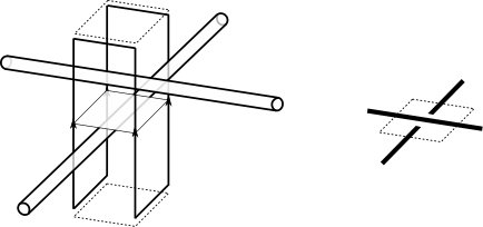 Figure 1
 Figure 2
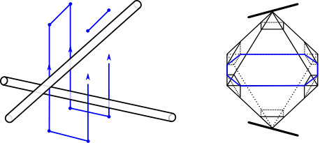 Figure 3
 Figure 4
 Figure 5
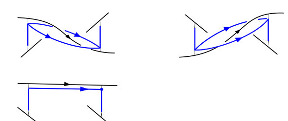 Figure 6
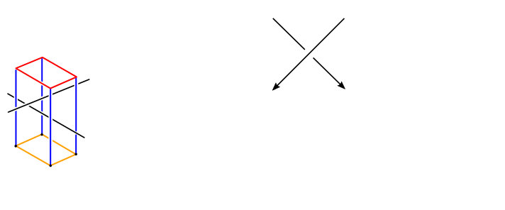 Figure 7
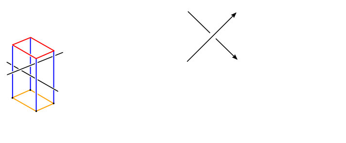 Figure 8
 Figure 9
 Figure 10
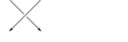 Figure 11
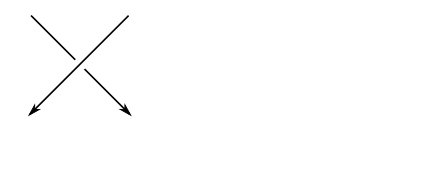 Figure 12
 Figure 13
 Figure 14
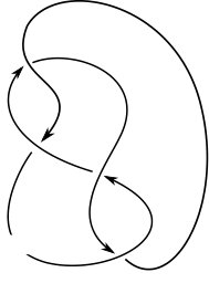 Figure 15
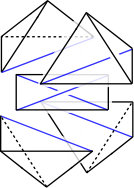 Figure 16
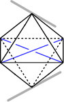 Figure 17
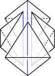 Figure 18
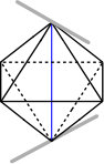 Figure 19
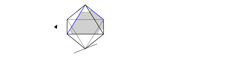 Figure 20
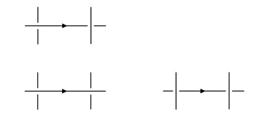 Figure 21
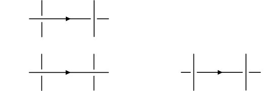 Figure 22
 Figure 23
 Figure 24
 Figure 25
 Figure 26
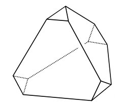 Figure 27
 Figure 28
 Figure 29
 Figure 30
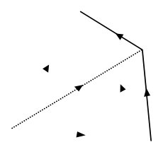 Figure 31
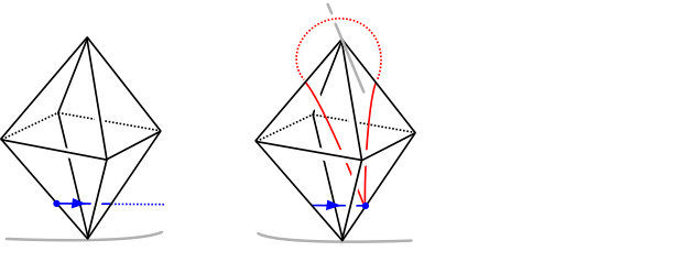 Figure 32
 Figure 33
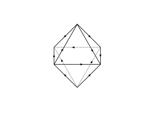 Figure 34
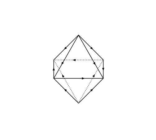 Figure 35
 Figure 36