Tensorization of the strong data processing inequality for quantum chi-square divergences
Yu Cao, Jianfeng Lu

TL;DR
This paper extends the tensorization property of strong data processing inequalities (SDPI) from classical to quantum channels, specifically for quantum chi-square divergences, enhancing understanding of quantum information contraction behaviors.
Contribution
It establishes the tensorization of SDPI constants for quantum chi-square divergences, a property previously known only in classical settings, for both quantum and quantum-classical channels.
Findings
Tensorization of SDPI constants for quantum chi-square divergences proven.
Applicable to arbitrary quantum channels and quantum-classical channels.
Enhances understanding of divergence contraction in quantum information theory.
Abstract
It is well-known that any quantum channel satisfies the data processing inequality (DPI), with respect to various divergences, e.g., quantum divergences and quantum relative entropy. More specifically, the data processing inequality states that the divergence between two arbitrary quantum states and does not increase under the action of any quantum channel . For a fixed channel and a state , the divergence between output states and might be strictly smaller than the divergence between input states and , which is characterized by the strong data processing inequality (SDPI). Among various input states , the largest value of the rate of contraction is known as the SDPI constant. An important and widely studied property for classical channels is…
Click any figure to enlarge with its caption.
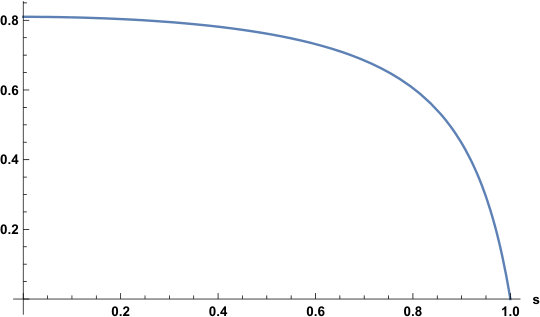 Figure 1
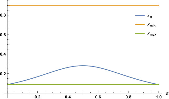 Figure 2
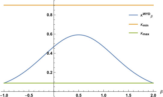 Figure 3
Peer Reviews
No public reviews on file for this paper yet. If you reviewed it on a platform where reviews are public (OpenReview, ICLR, NeurIPS, ICML), you can paste yours below so the community can read it here.
Videos
No videos yet. Explain this paper in a talk, walkthrough, or lecture? Add one.
Tensorization of the strong data processing inequality for quantum chi-square divergences
Yu Cao
Department of Mathematics, Duke University, Box 90320, Durham NC 27708, USA
Jianfeng Lu
Department of Mathematics, Duke University, Box 90320, Durham NC 27708, USA
Department of Physics and Department of Chemistry, Duke University, Box 90320, Durham NC 27708, USA
Abstract
It is well-known that any quantum channel satisfies the data processing inequality (DPI), with respect to various divergences, e.g., quantum divergences and quantum relative entropy. More specifically, the data processing inequality states that the divergence between two arbitrary quantum states and does not increase under the action of any quantum channel . For a fixed channel and a state , the divergence between output states and might be strictly smaller than the divergence between input states and , which is characterized by the strong data processing inequality (SDPI). Among various input states , the largest value of the rate of contraction is known as the SDPI constant. An important and widely studied property for classical channels is that SDPI constants tensorize. In this paper, we extend the tensorization property to the quantum regime: we establish the tensorization of SDPIs for the quantum divergence for arbitrary quantum channels and also for a family of divergences (with ) for arbitrary quantum-classical channels.
**Keywords: ** strong data processing inequality, tensorization, quantum chi-square divergence
1 Introduction
In information theory, the data processing inequality (DPI) has been an important property for divergence measures to possess operational meaning. For instance, DPI has been proved for quantum divergences (see e.g., [12, Thm. II.14] or [21, Thm. 4]), among other divergences. More explicitly, for any quantum channel and for all quantum states , we have
[TABLE]
In the above, is a real-valued positive function (see (7) below); the definition of divergences will be postponed to § 2.1, as it involves some technicalities.
Compared with the DPI, the strong data processing inequality (SDPI) quantitatively and more precisely characterizes the extent that quantum states contract under the channel [1, 18, 16, 17]. Given any -pair where is any quantum channel and is any full-rank quantum state ( is the space of strictly positive density matrices on a -dimensional Hilbert space), if there is a constant such that
[TABLE]
then the quantum channel is said to satisfy the strong data processing inequality (SDPI) for the quantum divergence and the smallest constant such that (2) holds is called the SDPI constant. Evidently,
[TABLE]
Many applications of SDPIs can be found in e.g., [17, Sec. 2.3] and [18, Sec. @slowromancapv@].
It is common in quantum information theory to consider high-dimensional quantum channels, formed by the tensor product of low-dimensional quantum channels. Except for very special cases, in general, obtaining SDPI constants for high-dimensional quantum channels can be rather challenging, even numerically. It is desirable if one could reduce the problem of calculating the SDPI constant for a (global) high-dimensional quantum channel, to calculating the SDPI constants of low-dimensional quantum channels. For a specific divergence (e.g., quantum divergence in this work), if the SDPI constant for the high-dimensional channel is the maximum value of SDPI constants for these low-dimensional channels, we say that the SDPI constant for this divergence satisfies the tensorization property.
Our main result in this work is that the SDPI constant for tensorizes, summarized in the following theorem.
Theorem 1**.**
Consider finite-dimensional quantum systems whose Hilbert spaces are with dimension () and consider any density matrix and any quantum channel acting on , such that for all , . If either of the followings holds
- (i)
; 2. (ii)
* and are quantum-classical (QC) channels;*
then we have the tensorization of the SDPI constant for the quantum divergence, i.e.,
[TABLE]
Remark**.**
- (i)
The function is a special example of weight functions. There are some properties that only the quantum divergence possesses (see e.g., Lemma 7 (ii)); in addition, is tightly connected to the sandwiched Rényi divergence of order [13].
There is a whole family of parameterized by , satisfying the condition ; see Example 3 for details; in § 2.2, we also present other examples of such that . The notion of QC channel will be recalled in § 2.6. 2. (ii)
These assumptions only provide sufficient conditions for the tensorization of SDPIs to hold, and it is an interesting open question to further investigate weaker conditions. In addition, it is also an interesting open question whether the tensorization of SDPIs holds for (quasi) relative entropies and the geodesic distances [12, 8]. We shall leave these questions to future research.
The tensorization property in the classical regime has been well studied and widely used; see e.g., [1, 22, 18]. For SDPI constants, the tensorization property was proved in [18, Thm. @[email protected]] for any -divergence, denoted by D_{\Phi}\left(\nu\mid\mid\mu\right):=\mathbb{E}_{\mu}\Big{[}\Phi(\frac{\,\mathrm{d}\nu}{\,\mathrm{d}\mu})\Big{]}-\Phi(1), provided that the associated -entropy is sub-additive and homogeneous. As a remark, the -divergence includes the relative entropy (with ) and the classical divergence (with ) as special instances. The tensorization of SDPI constants associated with the classical relative entropy has been applied to study the lower bounds of Bayes risk [24].
Establishing tensorization in the quantum regime seems to be more challenging and our understanding is much limited. Recently, the tensorization technique has been developed for the quantum hypercontractivity of qubit system [11], reversed hypercontractivity [7, 3], -log-Sobolev constant [10, 3], as well as the quantum maximal correlation [2]. For the tensorization of the quantum (reversed) hypercontractivity and log-Sobolev constants, all existing works, as far as we know, focus exclusively on reversible (or even more special) quantum Markov semigroups (i.e., Lindblad equations).
We would like to briefly mention and highlight the proof techniques used for Theorem 1. The first main ingredient is to formulate the SDPI constant as the second largest eigenvalue of a certain operator (see Lemma 10); similar results have been obtained in e.g., [5, 18, 20, 12, 8]. This result immediately leads into the proof of the case (i). The second main ingredient is to bound above by (see Lemma 12), whose proof uses Petz recovery map [14] as the bridge. This relation together with special properties of leads into the proof of case (ii).
Related techniques to quantify the loss of information
Apart from the DPI and the SDPI, there are other concepts used to characterize the contraction of quantum states under the action of noisy channels. For instance, one widely studied quantity is the contraction coefficient
[TABLE]
The contraction coefficient is very similar to the SDPI constant. However, compared with the SDPI constant, the contraction coefficient for various divergence measures has been much more extensively studied in the literature, see e.g., [20, 15, 12, 21, 8] for the quantum case, and see e.g., [6] for the classical case. The bijection maps that preserve the quantum divergence (see Example 3 about the family ) have been characterized in [4], which complements the study of the contraction of quantum states. There are other tools based on the functional perspective, including quantum (reverse) hypercontractivity and related quantum functional inequalities [10, 11, 7, 19, 3].
Contribution
We summarize new results obtained in this work, as follows:
- (i)
Our main result is Theorem 1, which establishes the tensorization of SDPI constants, under certain assumptions: for the quantum divergence, the tensorization of SDPI constants holds for general quantum channels; for the quantum divergence with , the tensorization holds for any quantum-classical channel. 2. (ii)
Along the analysis of the SDPI, we also establish a connection between the SDPI constant associated with and a variant of quantum maximal correlations; see Theorem 18 for details. 3. (iii)
To use the tensorization property, we need to understand the SDPI constants for local channels, i.e., we need to compute for . Motivated by this, we study the SDPI constants for special qubit channels in § 5. We notice that there is a particular QC channel associated with a fixed such that the largest value of for , while for (however, is close to a singular matrix); see § 5.1 for details. This extreme example shows the high dependence of SDPI constants on the choice of , which magnifies the difference between the quantum SDPI constant and its classical analog, because there is only one SDPI constant for the classical divergence.
This paper is organized as follows. In § 2, we provide some preliminary results, in particular, we recall the eigenvalue formalism of the SDPI constant. In § 3, we prove Theorem 1 and in § 4, we study the connection between the SDPI constant and the quantum maximal correlation. In § 5, we consider SDPI constants for qubit channels and study the dependence of on and . § 6 concludes the paper with some additional remarks.
2 Preliminaries
This section contains preliminary results that we will use to prove the tensorization of the strong data processing inequality, Theorem 1. In particular, we will present two variational formulations of SDPI constants, and discuss the relation between various SDPI constants.
Notations. We shall consider finite dimensional systems only, i.e., the Hilbert space . Let , , , be the space of linear operators, density matrices, strictly positive density matrices and Hermitian matrices on , respectively. Let and be the space of traceless elements of and , respectively. Denote the -by- identity matrix by (acting on ); let be the identity operator acting on . If the Hilbert space , and has the dimension (for ), then the space of linear operators on is denoted by ; the same convention applies similarly to other spaces, e.g., . As a reminder, following the above notation convention, .
Let denote a generic inner product on ; the Hilbert-Schmidt inner product is defined as . For any positive semidefinite operator on , define the sesquilinear form and the semi-norm for all ; when is strictly positive, the sesquilinear form becomes an inner product and the semi-norm becomes a norm.
For convenience, for any , we denote
[TABLE]
where and are left and right multiplication of and , respectively; in other words, .
2.1 Quantum divergences
Throughout this work, we consider the quantum divergence, introduced in [21, Def. 1]. Let us introduce a set ,
[TABLE]
As a remark, it is easy to check that is in the family .
Definition 2** (Quantum divergence).**
For any , define the quantum divergence between quantum states by
[TABLE]
when ; otherwise, set . The operator above is given by
[TABLE]
The second equality comes from the assumption that . As a remark, when is not a full-rank density matrix, can still be well-defined on the support of .
Essentially, the operator is a non-commutative way to multiply . Properties of the operator will be further discussed in § 2.3.
Next, let us introduce the non-commutative way to multiply . Define the weight operator
[TABLE]
Note that the operator is completely positive, with the Kraus operator and . For any , let us define a generalization of the operator
[TABLE]
Notice that .
2.2 Examples of
In this subsection, we provide three examples of such that (satisfying one of the conditions in Theorem 1). More examples can be found in [9, Sec. 4.2] and [8, Sec. (III)].
Example 3** (Quantum divergence).**
An important family of the quantum divergence is the quantum divergence, with the parameter and
[TABLE]
- (i)
The case is very special: and is completely positive with the Kraus operator . In fact, is the only one in such that for any , both and are completely positive [9, Theorem 3.5]. 2. (ii)
We can immediately verify that and for any fixed , is monotonically decreasing with respect to ; thus .
More results about this family of the quantum divergence (also called mean -divergence) could be found in [21].
Example 4** (Wigner-Yanase-Dyson).**
Another family of (see e.g., [8, 9]) corresponds to the Wigner-Yanase-Dyson metric, and it is parameterized by ,
[TABLE]
When , is simply set as or is defined by taking the limit in the above equation. In general, finding all possible such that seems to be slightly technical; however, at least, for a few special choices of , e.g., when () and () we can easily check that for these two cases.
Example 5** (The largest possible ).**
The largest is (see e.g., [8, Eq. (11)]). It is obvious that .
As a remark, in the family of Wigner-Yanase-Dyson metric is exactly the maximum one.
2.3 Basic properties of operators and
We list without proof some elementary while useful properties of the operator . Recall the assumption that , which is used below in the proof of being Hermitian-preserving.
Lemma 6**.**
Suppose and its eigenvalue decomposition . Then
- (i)
The operator can be decomposed as
[TABLE]
For any Hermitian matrix ,
[TABLE]
Thus, is a strictly positive operator with respect to the Hilbert-Schmidt inner product, and the inner product is well-defined. 2. (ii)
* is Hermitian-preserving.* 3. (iii)
We have . Thus for any ,
[TABLE]
In particular, for any density matrix , .
Then let us consider the properties of for a composite system.
Lemma 7**.**
- (i)
Consider and . Then for any and , we have
[TABLE] 2. (ii)
* is the only one in such that for all and , we have*
[TABLE]
Proof.
Let us decompose and , then has an eigenvalue decomposition .
- (i)
By the decomposition of the operator in (15),
[TABLE]
Then by direct calculation,
[TABLE]
The other case can be similarly proved. 2. (ii)
When , by the fact that , we can immediately see the tensorization (19). As for the other direction, from the assumption that (19) holds and after some straightforward simplification, one could obtain that , for all indices . Since and are arbitrary density matrices, we have for all ; in particular, . Since , we also have , which leads into .
∎
Similarly, we list without proof the following properties of ; all properties can be easily verified by the definition of in (11).
Lemma 8** (Operator ).**
Suppose and its eigenvalue decomposition . Then
- (i)
the operator for any has a decomposition
[TABLE]
thus is strictly positive with respect to the Hilbert-Schmidt inner product; 2. (ii)
the operator is Hermitian-preserving; 3. (iii)
.
2.4 Eigenvalue formalism of SDPI constants
The eigenvalue formalism of the quantum contraction coefficient can be found in e.g. [20, 12, 8]; the classical analogous result can be found in e.g., [5, 18]. In this subsection, we concisely present this formalism, for the sake of completeness.
Let us consider the ratio in the SDPI constant.
[TABLE]
where we introduce
[TABLE]
Here are some properties of the operator .
Lemma 9**.**
Assume that .
- (i)
The operator is positive semidefinite with respect to the inner product . 2. (ii)
. 3. (iii)
* is Hermitian perserving.* 4. (iv)
For any , we have
[TABLE]
Therefore, the eigenvalue of is bounded above by .
Proof.
Part (i) is obvious from (22) and Lemma 6 (i). Part (ii) can be verified directly by Lemma 6 (iii) and the fact that is trace-preserving (or equivalently is unital). As for part (iii), since the quantum channel is completely positive, it is thus also Hermitian-preserving; so is . By Lemma 6 (ii), is Hermitian-preserving, thus so is . Finally, since the composition of two Hermitian-preserving operators is also Hermitian-preserving, we conclude that is Hermitian-preserving. Part (iv) is essentially the data processing inequality; see e.g. [12, Thm. II.14] and [21, Thm. 4] for the proof. ∎
Then
[TABLE]
As one might observe, the last equation is closely connected to the eigenvalue formalism of the operator , which is stated in the following lemma.
Lemma 10**.**
For and and for any quantum channel such that , let be the second largest eigenvalue of (defined in (22)). Then
[TABLE]
Proof.
Since is positive semidefinite with respect to the inner product from Lemma 9 (i), it admits a spectral decomposition with where and is an orthonormal basis in the Hilbert space . Note that is always an eigenvector of from Lemma 9 (ii); without loss of generality, let and . By the orthogonality of , we know for . By Lemma 9 (iv), for all ; thus without loss of generality, assume are listed in descending order and hence . By rewriting in (23) where , we immediately know that .
By the fact that is Hermitian-preserving (see Lemma 9 (iii)), is also an eigenvector associated with the eigenvalue . Then we choose in (23) by or . Note that such an is also an eigenvector of with the eigenvalue . Then ∎
2.5 Another variational formalism of SDPI constants
Recall the definition of the operator from (12). In Lemma 11 below, we provide another variational characterization of the SDPI constant; essentially, it follows from the connection between the eigenvalue formalism (as discussed in the last subsection) and the corresponding singular value formalism. Its classical version is well-known and can be found in e.g. the proof of [18, Thm. @[email protected]]. This idea for quantum divergences has appeared implicitly in [21, Thm. 9]; however, we don’t assume to be the stationary state of the quantum channel herein, compared with [21].
Lemma 11**.**
Assume that quantum states . For any ,
[TABLE]
where the operator is defined by
[TABLE]
and the maximum is taken over all such that
[TABLE]
Proof of Lemma 11.
First, we rewrite Lemma 10 in the language of the relative density (whose classical analog is the Radon–Nikodym derivative); specifically, to get the third equality below, is replaced by . By Lemma 10,
[TABLE]
As for the operator , it can be straightforwardly checked that
- •
is completely positive and unital ().
- •
is completely positive, trace-preserving, and .
- •
Consider the following two Hilbert spaces and ,
[TABLE]
Then we can readily verify that is an operator from to , i.e., if , then . The dual operator of , denoted by , maps from to and it is explicitly given by .
Then, we have
[TABLE]
Let us denote the SVD decomposition of by where , and are orthonormal basis of and respectively. Then, easily we know and that . Then is simply the largest value of ; namely, is the largest singular value of , and the result in Lemma 11 follows immediately. ∎
2.6 Comparison of SDPI constants
First, we provide a uniform lower bound of for any in terms of in Lemma 12, which is a new result to the best of our knowledge. One of our corollaries in (30) can also be derived by [8, Thm. 4.4] and [8, Thm. 5.3]. However, our approach to show (30) is different from [8]: their result comes from comparing the contraction coefficient with (the contraction coefficient for trace norm); we use the SDPI constant of the Petz recovery map as the bridge. Second, we consider quantum-classical (QC) channels and provide the ordering of SDPI constants for different in Lemma 14; similar results have appeared in [8, Prop. 5.5] for contraction coefficients.
Lemma 12**.**
For any quantum channel and quantum state such that , we have
[TABLE]
where is the Petz recovery map, defined by
[TABLE]
mapping to .
The followings are immediate consequences of the lemma above.
Corollary 13**.**
Under the same assumption as in Lemma 12,
- (i)
The SDPI constant associated with for the pair equals the SDPI constant for the recovery map pair , that is to say,
[TABLE] 2. (ii)
Further assume that for any , we have . Then, for the contraction coefficient of the quantum channel , we have
[TABLE]
Proof.
The first part comes from letting in (28) and the fact that the Petz recovery map of is exactly the channel ; the second part comes from taking the supremum over all . ∎
Proof of Lemma 12.
It is straightforward to verify that , defined in (29), is a bona-fide quantum channel, mapping the quantum state back to . We can easily verify by definition (22) and (29) that
[TABLE]
Recall from Lemma 10 that there exists a and a traceless Hermitian matrix such that . Let . Then
[TABLE]
The inequality in the last step follows from Lemma 10. Hence, we have proved the first inequality in (28); the second inequality follows immediately from the data processing inequality of the quantum divergence. ∎
Next, we consider any quantum-classical (QC) channel , which refers to a physical process in which one first performs a measurement according to a POVM ( are positive semidefinite and ); then based on the measurement outcome, one prepares a pure state, selected from a set which also forms an orthonormal basis of . More specifically,
[TABLE]
Define a ratio on by
[TABLE]
Lemma 14**.**
Suppose , is a QC channel with for all and . Then
[TABLE]
Consequently, we have
[TABLE]
Proof.
By (32) and (16), we can readily calculate that
[TABLE]
which is independent of . By (16), it is straightforward to observe that when , one has . Thus (34) follows immediately; (35) follows from (34) by taking the supremum over all non-zero (see (23)). ∎
3 Proof of Theorem 1
Setting up: First notice that it is sufficient to prove Theorem 1 for . The general case can be straightforwardly proved by mathematical induction on . Next, for the case , one direction is trivial: suppose achieves the maximum in ; let and by direct calculation,
[TABLE]
Similarly, by choosing where achieves the maximum in , we have . Therefore,
[TABLE]
In the below, we shall prove the other direction, i.e.,
[TABLE]
Notations:
Since we fix states and channels for throughout this section, let us denote for simplicity of notation. By Lemma 10, has an eigen-basis associated with eigenvalue with respect to the inner product such that
[TABLE]
where , and are Hermitian for all , since from Lemma 9 are both Hermitian-preserving positive semidefinite operators. In addition, we know from Lemma 10 (or say Lemma 9 (iv)) that for both ,
[TABLE]
For convenience, let and ; let . For any index pair , define
[TABLE]
Case (@slowromancapi@): For and any quantum channel. From Lemma 7 part (ii), tensorizes, thus . Next, we can straightforwardly verify that (for ) is an orthonormal eigenbasis of with respect to the inner product , and the associated eigenvalues are . The largest eigenvalue of on the domain becomes . Therefore, by Lemma 10, we have Thus we complete the proof of (37) for the case .
Case (@slowromancapii@): For and QC channels. Let us decompose by where . From the constraint that , we know . Thus, we can rewrite A by
[TABLE]
where
[TABLE]
To prove (37), by (23), it is equivalent to prove that for all and , we have
[TABLE]
The next lemma shows that it is sufficient to consider A as .
Lemma 15**.**
If (40) holds for any , then (40) holds for any .
Notice that . The proof of this lemma is postponed to the end of this section and let us continue to complete the proof of Theorem 1. It is straightforward to verify that when and are QC channels, is also a QC channel for the composite system. By Lemma 14, for any , we have
[TABLE]
The second inequality comes from the observation that is a positive semidefinite operator on the space with eigenvalues ; for and , recall from previous results that . The last equation means (40) holds for all Hermitian and by Lemma 15, (40) holds for all Hermitian . This completes the proof of Theorem 1.
Proof of Lemma 15..
For any Hermitian A in (38), we claim that
[TABLE]
To prove this, we need to show that all cross product terms in the expansion of vanish. For instance, consider any ,
[TABLE]
If or , by plugging the expression of or into the last equation and after expanding all terms, it is straightforward to verify that for both choices of B. We can apply similar arguments to for or . Similarly, we have (or let in (41))
[TABLE]
Let us simplify the term on the right hand side of (41). For instance,
[TABLE]
Similarly,
[TABLE]
Therefore, we have
[TABLE]
By comparing (42) and (43), to prove (40), it is sufficient to show
[TABLE]
Thus we complete the proof of Lemma 15.
∎
4 Connection to the quantum maximal correlation
The SDPI constant for the classical divergence is closely connected to the classical maximal correlation (see e.g., [18, Theorem @[email protected]]). In the proposition below, we provide a quantum analog of this relation when .
To begin with, we need to define the quantum maximal correlation. This concept was previously proposed and studied in [2]. Since there is a whole family of quantum divergences, it is natural to imagine that there could also exist a whole family of quantum maximal correlations, as a straightforward generalization of [2].
Definition 16** (-quantum maximal correlation).**
Consider any fixed and Hilbert spaces and with dimensions and respectively. For any bipartite quantum state on the composite system , denote the reduced density matrices by and respectively (i.e., , ). Define the -quantum maximal correlation by
[TABLE]
where the maximum is taken over all , such that
[TABLE]
Technically, when is not a full-rank density matrix, the notation should be understood as a sesquilinear form, as we explained at the beginning of § 2 and the operator is still well-defined on the support of via (20).
By Lemma 8, we easily verify that and . When is a constant function, we recover the quantum maximal correlation defined in [2]; in this case, ; however, notice that this choice of is not included in the set and the corresponding operator is not Hermitian-preserving.
Lemma 17** (Invariance of the -quantum maximal correlation under local isometries).**
Suppose and are two isometries (i.e., and ), where and . For any bipartite quantum state on , define . We have
[TABLE]
Proof.
By definition,
[TABLE]
where we define and . Denote the reduced density matrices of as and respectively. Then the reduced density matrices of are given by and respectively. From (46), the condition in the maximization is given by
[TABLE]
By (20), it could be readily shown that and similarly for . As a remark, in this case, and might not be strictly positive, then the decomposition in (20) only considers eigenstates with respect to non-zero eigenvalues (i.e., is only defined on the support of ). Then, with direct calculation, one could verify that the above four conditions are equivalent to
[TABLE]
Therefore, we know . Since is a linear operator on a higher-dimensional Hilbert space than on , for any such , there exists such that (similarly for ); therefore the equality can be achieved and . ∎
Theorem 18**.**
For a Hilbert space with dimension , suppose and is any quantum channel on such that the quantum state . Thus, has an eigenvalue decomposition For the choice ,
[TABLE]
where the bipartite quantum state and the wave function is any purification of on the system .
Recall that a pure state on is a purification of if (see [23, Chap. 5]). The canonical choice of the purification of is
[TABLE]
Proof.
In the first step, we prove it for the choice ; in the second step, we extend the result to the general purification.
Step (@slowromancapi@). By Lemma 11, we have
[TABLE]
where . Let us decompose based on the eigenstates of ,
[TABLE]
Hence,
[TABLE]
where and the superscript means transpose with respect to the eigenstates of , i.e., for all . The last equality above can be verified directly by .
Notice that from Lemma 11, the maximum is taken over all given in (27). Hence, to prove Theorem 18, it remains to verify that conditions (27) for and are equivalent to conditions (46) for and . More specifically, we need to verify the following four relations.
- (i)
. Note that
[TABLE] 2. (ii)
. Note that
[TABLE] 3. (iii)
. Note that
[TABLE] 4. (iv)
. Note that
[TABLE]
When , . Thus the relation holds for this special choice of and this is the only place we employ this assumption.
Step (@slowromancapii@): We then extend the result from the canonical purification to any purification on the bipartite quantum system . By [23, Theorem 5.1.1], there exists a unitary (thus also isometry) such that . Hence, . By Lemma 17, the conclusion follows immediately. ∎
5 SDPI constants for special qubit channels
In this section, we will illustrate the dependence of SDPI constants on the reference state and the weight function , for several special qubit channels. The dependence on is one major difference between the quantum SDPI framework and the quantum contraction coefficient approach. The dependence on is one major difference between the quantum SDPI framework and its classical version: all quantum divergences coincide for classical states and (i.e., and commute) and simply reduce to the classical divergence; in particular, classical divergence, as well as the associated classical SDPI constant, does not depend on ; however, the SDPI constant for quantum divergences might fluctuate significantly between approximately [math] and for various , in a special example that we provide below.
Three Pauli matrices are denoted by . Without loss of generality, assume \sigma=\frac{1}{2}\left(\mathbb{I}_{2}+s\sigma_{Z}\right)=\mathopen{\big{missing}}[\begin{smallmatrix}(1+s)/2&0\\ 0&(1-s)/2\end{smallmatrix}\mathclose{\big{missing}}] with , because one can always choose the eigenbasis of as the computational basis; of course, the matrix representation of the quantum channel is changed, by choosing such a specific computational basis.
5.1 QC channel
By the expression of QC channel (32) and by (36), we have for any that
[TABLE]
The second equality comes from the fact that and . Let us decompose and ; notice that all coefficients for and are real numbers. Next, rewrite the above equation by
[TABLE]
From (16), we also have
[TABLE]
where
[TABLE]
By the Cauchy–Schwarz inequality and the fact that and , we have
[TABLE]
Hence, we know that
[TABLE]
As we can observe, the SDPI constant depends on and the parameter in a complicated way; however, it does not depend on the choice of pure states in the post-measurement preparation in (32). In the following, let us consider a few special choices of the POVM .
(High dependence on , for the quantum implementation of BSC)
If (thus ) with , then the channel is exactly a quantum implementation of the binary symmetric channel with crossover probability (or BSC() in short). Easily, we know , , and thus the SDPI constant can be simplified as
[TABLE]
Notice that the SDPI constant in this case is independent of the choice of ; the upper bound comes from the fact that . When we further let , i.e., the reference state has the distribution Bern(), the SDPI constant achieves the upper bound , which recovers [18, Example @[email protected]]. In Figure 1, we show with respect to the parameter in , for fixed ; the high dependence of on (i.e., on ) can be clearly seen, for this particular case.
(High dependence on ).
If with , then , and . Hence,
[TABLE]
The inequality comes from the fact for any , we have (see [8, Eq. (11)]). As one could observe, even for this simple example, the dependence of on and is nonlinear and slightly complicated. Similarly, by the fact that for any , we have (see [8, Eq. (11)]), one could immediately show that
[TABLE]
Notice that both upper and lower bounds in the above can be achieved for some . When and , the largest value of is approximately , while the smallest value is approximately [math], which illustrates the high dependence of on the choice of , for this extreme case. In Figure 2, we visualize the SDPI constant with respect to various choices of , for ; the high dependence of on can be clearly observed.
5.2 Depolarizing channel
The depolarizing channel on a qubit has the following form
[TABLE]
for . It refers to a physical process in which for a given input state , one prepares with probability and prepares the maximal mixed state with probability . Easily, we know that , and for any . Hence,
[TABLE]
If , then
[TABLE]
For fixed and , might be largely affected by as well.
6 Conclusion and outlook
In this paper, we provide a partial solution to the problem of the tensorization of SDPIs for quantum channels in Theorem 1. In addition, we extend the connection between the SDPI constant for classical divergence and the maximal correlation to the quantum region in Theorem 18. For a particular QC channel and a special quantum state , we observe an extreme scenario, in which the SDPI constant ranges approximately from [math] to for different . This implies that choosing different might largely affect the rate of contraction of quantum channels. Our numerical experiments (not presented in the paper) conducted for both qubit (i.e., ) and qudit (with ) systems show that the tensorization property (4) seems to hold for any quantum channel , any reference state and at least a few weight functions being tested (e.g., , and the family with and ). Proving such tensorization properties is an interesting future work.
Finally, let us comment on the potential generalization of our approach, as well as the limitation. As one might observe, provided that one could show (34), the tensorization of SDPIs is an immediate consequence. However, it seems to be challenging to characterize the class of quantum channels that satisfy (34) in general and this is the reason why we restrict to QC channels and the case in Theorem 1. In terms of the validity of (34), we notice that when (e.g., ), (34) does not hold even for QC channels. As mentioned above, numerical experiments seem to suggest that the tensorization also holds for . Therefore, further understanding of the properties of quantum divergences is needed to extend our results.
Acknowledgment
This work is supported in part by the US National Science Foundation via grants DMS-1454939 and CCF-1910571 and by the US Department of Energy via grant DE-SC0019449. We thank Iman Marvian and Henry Pfister for helpful discussions. Iman Marvian pointed out the possible generalization of Theorem 18 from the canonical purification to any general purification. Henry Pfister introduced us to the topic of the strong data processing inequality for classical noisy channels. We also thank anonymous referees for helpful suggestions.
The reference list from the paper itself. Each links out to its DOI / PubMed record.
- 1Anantharam et al. [2013] Venkat Anantharam, Amin Gohari, Sudeep Kamath, and Chandra Nair. On maximal correlation, hypercontractivity, and the data processing inequality studied by Erkip and Cover, Apr 2013. ar Xiv:1304.6133.
- 2Beigi [2013] Salman Beigi. A new quantum data processing inequality. J. Math. Phys. , 54(8):082202, 2013. doi: 10.1063/1.4818985 .
- 3Beigi et al. [2018] Salman Beigi, Nilanjana Datta, and Cambyse Rouzé. Quantum reverse hypercontractivity: its tensorization and application to strong converses, Apr 2018. ar Xiv:1804.10100.
- 4Chen et al. [2017] Hong-Yi Chen, György Pál Gehér, Chih-Neng Liu, Lajos Molnár, Dániel Virosztek, and Ngai-Ching Wong. Maps on positive definite operators preserving the quantum χ α 2 subscript superscript 𝜒 2 𝛼 \chi^{2}_{\alpha} -divergence. Lett. Math. Phys. , 107(12):2267–2290, 2017. doi: 10.1007/s 11005-017-0989-0 .
- 5Choi et al. [1994] Man-Duen Choi, Mary Beth Ruskai, and Eugene Seneta. Equivalence of certain entropy contraction coefficients. Linear Algebra Appl. , 208-209:29–36, 1994. doi: 10.1016/0024-3795(94)90428-6 .
- 6Cohen et al. [1993] Joel E. Cohen, Yoh Iwasa, Gh. Rautu, Mary Beth Ruskai, Eugene Seneta, and Gh. Zbaganu. Relative entropy under mappings by stochastic matrices. Linear Algebra Appl. , 179:211–235, 1993. doi: 10.1016/0024-3795(93)90331-H .
- 7Cubitt et al. [2015] Toby Cubitt, Michael Kastoryano, Ashley Montanaro, and Kristan Temme. Quantum reverse hypercontractivity. J. Math. Phys. , 56(10):102204, 2015. doi: 10.1063/1.4933219 .
- 8Hiai and Ruskai [2016] Fumio Hiai and Mary Beth Ruskai. Contraction coefficients for noisy quantum channels. J. Math. Phys. , 57(1):015211, 2016. doi: 10.1063/1.4936215 .