Multi-d Isothermal Euler Flow: Existence of unbounded radial similarity solutions
Helge Kristian Jenssen, Charis Tsikkou

TL;DR
This paper demonstrates the existence of global, radially symmetric solutions with unbounded amplitudes in the multi-dimensional isothermal Euler system, highlighting wave focusing phenomena and expanding shock waves in ideal gas flows.
Contribution
It constructs explicit similarity solutions showing unbounded behavior in the isothermal Euler system, a novel result contrasting with classical Guderley solutions.
Findings
Existence of unbounded radial solutions due to wave focusing.
Density becomes unbounded at collapse, velocity remains bounded.
Solutions verified as genuine weak solutions to the system.
Abstract
We show that the multi-dimensional compressible Euler system for isothermal flow of an ideal, polytropic gas admits global-in-time, radially symmetric solutions with unbounded amplitudes due to wave focusing. The examples are similarity solutions and involve a converging wave focusing at the origin. At time of collapse, the density, but not the velocity, becomes unbounded, resulting in an expanding shock wave. The solutions are constructed as functions of radial distance to the origin and time . We verify that they provide genuine, weak solutions to the original, multi-d, isothermal Euler system. While motivated by the well-known Guderley solutions to the full Euler system for an ideal gas, the solutions we consider are of a different type. In Guderley solutions an incoming shock propagates toward the origin by penetrating a stationary and "cold" gas at zero pressure (there is…
Click any figure to enlarge with its caption.
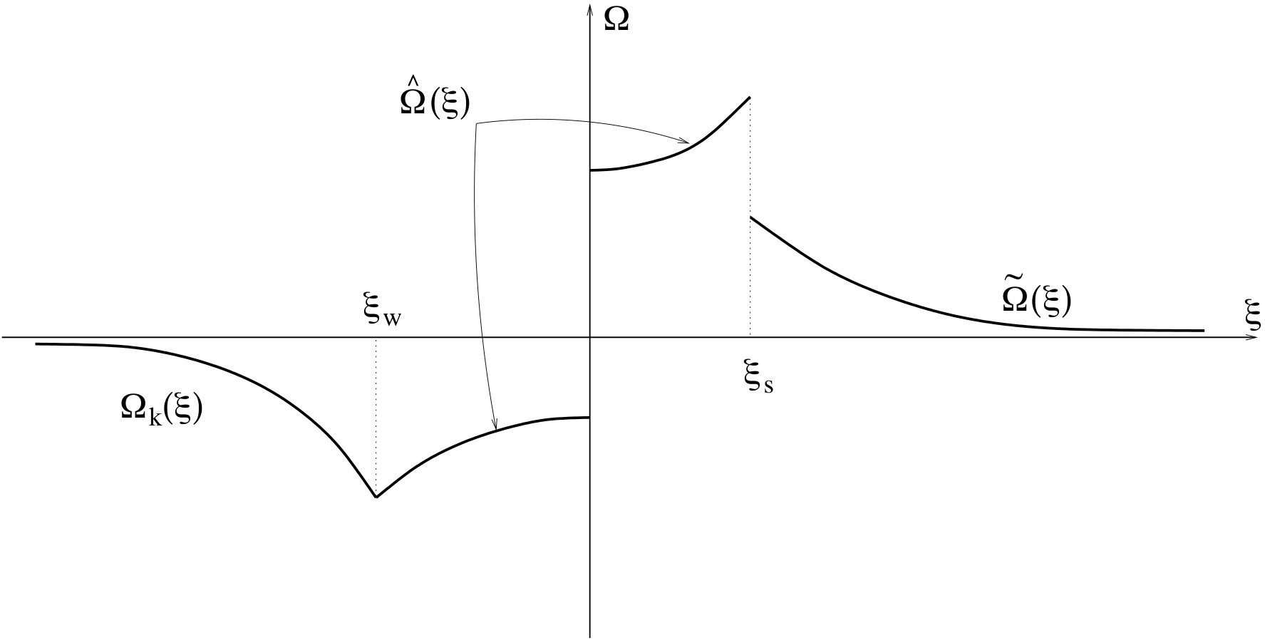 Figure 1
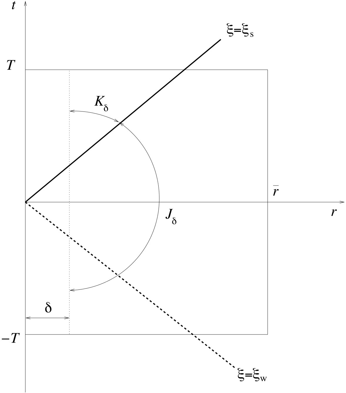 Figure 2
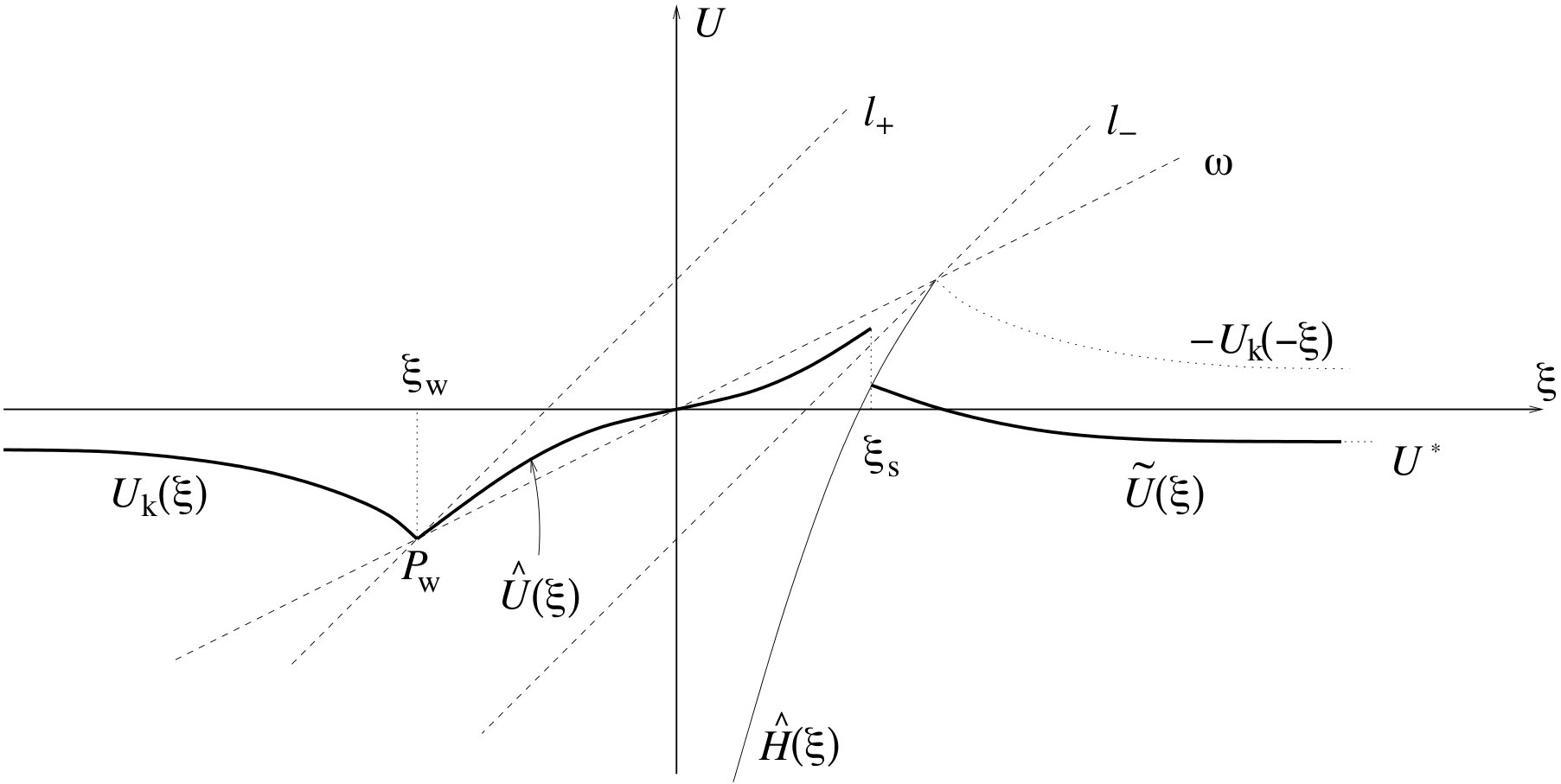 Figure 3
Peer Reviews
No public reviews on file for this paper yet. If you reviewed it on a platform where reviews are public (OpenReview, ICLR, NeurIPS, ICML), you can paste yours below so the community can read it here.
Videos
No videos yet. Explain this paper in a talk, walkthrough, or lecture? Add one.
Multi-d Isothermal Euler Flow: Existence of unbounded radial similarity solutions
Helge Kristian Jenssen
H. K. Jenssen, Department of Mathematics, Penn State University, University Park, State College, PA 16802, USA ([email protected]).
and
Charis Tsikkou
C. Tsikkou, Department of Mathematics, West Virginia University, Morgantown, WV 26506, USA ([email protected]).
Abstract.
We show that the multi-dimensional compressible Euler system for isothermal flow of an ideal, polytropic gas admits global-in-time, radially symmetric solutions with unbounded amplitudes due to wave focusing. The examples are similarity solutions and involve a converging wave focusing at the origin. At time of collapse, the density, but not the velocity, becomes unbounded, resulting in an expanding shock wave. The solutions are constructed as functions of radial distance to the origin and time . We verify that they provide genuine, weak solutions to the original, multi-d, isothermal Euler system.
While motivated by the well-known Guderley solutions to the full Euler system for an ideal gas, the solutions we consider are of a different type. In Guderley solutions an incoming shock propagates toward the origin by penetrating a stationary and “cold” gas at zero pressure (there is no counter pressure due to vanishing temperature near the origin), accompanied by blowup of velocity and pressure, but not of density, at collapse. It is currently not known whether the full system admits unbounded solutions in the absence of zero-pressure regions. The present work shows that the simplified isothermal model does admit such behavior.
Contents
-
2 Rankine-Hugoniot and Entropy conditions for similarity flows
-
6 Radial converging-diverging similarity solutions as weak solutions
1. Equations
The compressible Euler system for barotropic flow in is given by
[TABLE]
where the independent variables are time and position , and the primary dependent variables are density and velocity , while pressure is a given function of density, . In isothermal flow of an ideal, polytropic gas the pressure is a linear function of density:
[TABLE]
For radial ( spherically symmetric) solutions the dependent variables are functions of time and radial distance to the origin, and the velocity field is purely radial: . In this case (1.1)-(1.2) reduces to a quasi one-dimensional system:
[TABLE]
where . For smooth (Lipschitz) flows this reduces further to
[TABLE]
In this work we shall be concerned exclusively with complete radial isothermal flows of similarity type. This means and are defined for all , , and are of the form
[TABLE]
where the similarity variable is given by
[TABLE]
A discussion of our results and their relations to earlier works appears in Section 3.
At this stage in (1.8) is a free parameter. Substitution of (1.3) and (1.8) into (1.6)-(1.7) yields the similarity ODEs (where )
[TABLE]
Solving for in (1.10) and substituting into (1.9) yield a single ODE for :
[TABLE]
Using this in (1.10) gives
[TABLE]
Before analyzing the similarity ODEs we consider the jump conditions in similarity variables.
2. Rankine-Hugoniot and Entropy conditions for similarity flows
Consider the radial barotropic Euler system (1.4)-(1.5), and assume that a discontinuity propagates along the path . The Rankine-Hugoniot conditions are then
[TABLE]
where . Here and below we use the convention that, for any quantity , \big{[}\!\!\big{[}q\big{]}\!\!\big{]} denotes the jump in as decreases, i.e.,
[TABLE]
Next, denoting the local sound speed by
[TABLE]
the entropy condition for a 1-shock requires that
[TABLE]
while the entropy condition for a 2-shock requires that
[TABLE]
2.1. Radial isothermal similarity shocks
We next specialize to “similarity shocks” in radial isothermal flow: the pressure law is given by (1.3) and the shock is assumed to propagate along a path of the form , i.e., . Furthermore, it is assumed that the density and velocity on either side of the shock are of the form (1.8), with taking the same value on both sides. Let and denote the parts of the solution on the outside and inside of the shock, respectively. (“Outside” and “inside” refer to further away from and closer to , respectively.)
The Rankine-Hugoiniot conditions reduce to
[TABLE]
where \big{[}\!\!\big{[}\cdot\big{]}\!\!\big{]} now denotes jump across . The entropy conditions (2.3)-(2.4) take the form
[TABLE]
In particular, these relations show that for any shock in radial isothermal flow, the velocity necessarily decreases as we traverse the shock from the inside to the outside.
Finally, setting , where denotes , the Rankine-Hugoniot conditions take the form \big{[}\!\!\big{[}\Omega V\big{]}\!\!\big{]}=0 and \big{[}\!\!\big{[}\Omega VU+a^{2}\Omega\big{]}\!\!\big{]}=0. It follows from these that , and that
[TABLE]
Alternatively, solving for and , we have
[TABLE]
3. Converging-diverging isothermal flows
By a “converging-diverging solution” we shall mean a radial similarity solution in which a wave approaches the origin, “collapses” there at some instant in time, resulting in a reflected wave moving away from the origin. Without loss of generality we set the time of collapse to be .
We shall search for this type of solutions within the class of isothermal similarity solutions introduced above. To be of physical interest the solutions should satisfy, as a minimum, the following requirements:
- (A)
the velocity vanishes along : ;
- (B)
at any fixed location , the limits
[TABLE]
both exist as finite numbers. (Note that this requirement leaves open the possibility that and/or may blow as .)
In addition we shall require that the density field is everywhere strictly positive:
- (C)
the density never vanishes: for all , .
Further constraints will be imposed later to guarantee that the solutions, as function of , provide genuine weak solutions of the original, multi-d isothermal system (1.1)-(1.2). In particular, we shall require that the conserved quantities map time continuously into ; see Section 5 and also Section 7.
For the full Euler system (including conservation of energy) the seminal work [gud] by Guderley established the existence of converging-diverging similarity solutions in which a shock wave propagates into a quiescent state near the origin, focuses (collapses) at the origin, and reflects an expanding shock wave. Building on the detailed work of Lazarus [laz] (which also treats the case of a collapsing vacuum), the present authors recently showed in [jt1] that these “Guderley solutions” provide examples of genuine, entropy admissible, weak solutions to the full, multi-d Euler system. A key feature of these converging-diverging shock solutions is that they provide concrete Euler flows suffering pointwise blowup of primary flow variables (as opposed to blowup of their gradients).
Although the Guderley solutions establish the possibility of amplitude blowup in Euler flows for ideal gases, they are also at the borderline of the regime where one would expect the Euler system to be physically accurate. More precisely, in order to provide an exact weak solution, the sound speed in the quiescent state that the incoming shock moves into must vanish. For the ideal gas case under consideration, this means that the incoming shock does not experience any upstream counter-pressure. (The gas is at zero temperature there and this is sometimes referred to as a “cold gas assumption.”) It appears reasonable that this lack of counter-pressure facilitates unbounded growth of the shock speed, with concomitant increases in pressure and temperature. It is unclear at present whether this is the (or part of the) mechanism driving the blowup in Guderley solutions for the full Euler system. The alternative is that the blowup is a purely geometric effect driven by wave focusing, much like what occurs for radial solutions of the linear, multi-d wave equation.
The main goal of the present work is to show that amplitude blowup can occur in converging-diverging flows for the simplified isothermal Euler model, even in the presence of an everywhere strictly positive pressure field. To the best of our knowledge, the solutions we generate are the first examples of unbounded barotropic flows that meet the requirements (A)-(C) above. While these isothermal solutions are qualitatively different from the Guderley solutions for the full system described earlier (in particular, they are continuous up to collapse), they indicate that the real agent for blowup is the focusing of waves at the center of motion. On the other hand, it still remains an open problem to exhibit concrete flows for the full Euler system that exhibit blowup in the absence of zero-pressure regions.
For completeness we include some remarks on what is known about radial Euler flows with “general” initial data. First, there is currently no result for the full, multi-d Euler system, radial or not, that guarantees global-in-time existence. For radial isentropic flows, i.e., solutions to (1.4)-(1.5) with and , results by Chen-Perepelitsa [cp] and Chen-Schrecker [cs] provide existence of weak, finite energy solutions via the method of compensated compactness. In fact, the recent work [sch] is the first to show that the solutions one obtains in this manner provide genuine, weak solutions to the original, multi-d isentropic Euler system (1.1)-(1.2) on all of space. On the other hand, there appears to be little hope of extending this approach (i.e., compensated compactness) to the radial full system, or even (for technical reasons [sch1]) to the radial, isothermal () system.
As far as we know, the currently strongest, global existence result for the radial isothermal system applies to the case of external flows, i.e., for flows outside of a fixed ball. This problem was analyzed in [mmu1] by exploiting the Glimm scheme, providing existence for a certain class of initial data of bounded variation; for an extension, see [mmu2]. The results of the present paper shows that, in order to extend these results to solutions defined on all of space (i.e., including the origin), one must necessarily contend with unbounded solutions.
For results closer to the present work, which concerns concrete Euler flows in several space dimensions, see Chapter 7 of Zheng’s monograph [zheng] on multi-d Riemann problems, some of which generate purely radial flows. However, we stress that the radial flows we construct below are not solutions to Riemann problems. Specifically, the solutions we display are necessarily non-constant in the radial direction at all times.
The rest of the present paper is organized as follows. Section 4 provides a detailed construction of the radial speed and the corresponding density for converging-diverging similarity flows for the isothermal Euler system. In Section 5 we briefly recall the definition of weak solutions to the barotropic Euler system, including its formulation for the special case of radial solutions. In Section 6 we verify that the radial similarity flows we construct provide genuine weak solutions to the original, multi-d isothermal Euler system. The main result is summarized in Theorem 6.1. Finally, Section 7 collects some additional observations about the flows constructed in this paper.
4. Construction of converging-diverging isothermal flows
To construct concrete examples of converging-diverging isothermal similarity flows, we start with the ODE (1.11) for the velocity . This ODE has three critical points: the origin and the points , where
[TABLE]
(The subscript “w” stands for “weak,” for reasons to be clear later.) We also observe that its solutions are symmetric about the origin: if is a solution of (1.11), so is .
Instead of performing a lengthy analysis of all possible cases, from now on we focus on the cases where
[TABLE]
In particular, and for all cases under consideration. Introducing the straight lines
[TABLE]
we have that . Linearizing (1.11) about the critical points , we set
[TABLE]
where
[TABLE]
It is immediate to verify that the radicand in (4.2) is strictly positive whenever (4.1) holds. An analysis of the critical points shows that:
- (a)
The point is an unstable node for (1.11) whenever (4.1) holds, i.e., we have . 2. (b)
There are two solutions leaving along the directions . 3. (c)
All other solutions leaving do so along the directions . 4. (d)
Whenever (4.1) holds we have and ; thus all but the two solutions described in (b), enter the region between the straight lines and . 5. (e)
There is a unique solution passing through ; it does so with slope , and this solution is located below and above ; it extends back (i.e., as decreases) to , approaching along the direction .
We denote the unique solution described in (e) by . It passes through the origin and, by symmetry about the origin, is defined for all , and connects to the third critical point . See Figure 1.
4.1. The radial speed for
The part of corresponding to yields, via (1.8)2, the radial speed within the sector
[TABLE]
in the -plane. Note that the choice of the solution in this region is dictated by requirement (A) above. Similarly, we shall use a certain portion of for to obtain the radial speed within a sector
[TABLE]
Here the value of , yet to be determined, corresponds to the path of an expanding shock wave for .
However, we first need to continue the relevant -solution beyond , all the way down to . Now, there are infinitely many solutions of (1.11) defined for all , passing through , and with the property that they enter (as decreases) the region to the left of and above , i.e.,
[TABLE]
Let denote any such solution. We therefore have an infinity of choices for . As we shall see below, all of these solutions (that enter at points along ) tend to finite limits at , as dictated by the first part of requirement (B) above. However, it will be convenient for the subsequent analysis to also have . We proceed to show that there are solutions satisfying this constraint, as well as the constraints in (4.1).
4.1.1. Asymptotics for large, negative -values.
As is clear from the linearization of (1.11) at , all but one of the solutions defined on approach along ; all of these connect smoothly at with the solution on considered above. The exception is the “kink-solution” which approaches along . It is clear that lies above any solution of (1.11) which is located in and which exits (as increases) at a point on . For our purpose of having , it therefore suffices to identify cases for which tends to a strictly negative limit at , and then employ in our construction of within the sector
[TABLE]
We start by observing that for we have so that
[TABLE]
Therefore, any solution of (1.11) in satisfies
[TABLE]
Specializing to the kink-solution , which satisfies for , we obtain
[TABLE]
Integrating from to , and using that , yields
[TABLE]
Therefore, whenever and satisfy , and are such that the right-hand side of (4.3) is non-positive, then the kink-solution tends to a strictly negative limit as . E.g., with and , the right-hand side of (4.3) takes the value zero, while for and it takes a strictly negative value.
Assumption 1**.**
From now on it is assumed that and are such that or , , and at the same time
[TABLE]
the argument above demonstrates that such values of and exist.
As indicated above, we use the kink-solution to specify the radial speed , via (1.8)2, within the sector
4.2. The radial speed for ; the reflected shock.
Next, we need to specify the radial speed within the sector
[TABLE]
where is yet to be determined. The relevant solution of (1.11) (i.e., which is defined for ) should give a radial speed which is continuous across . It follows that must be the solution to (1.11) which approaches the value as .
Now, as we integrate along decreasing -values, in from , the solution remains below the solution . This follows since the latter function is a solution of (1.11) (recall that solutions of (1.11) lie symmetrically about the origin), and that it starts out from with the value . As a consequence we have that the solution intersects the straight line at some -value with .
Finally, to determine the shock location we argue as follows. Returning to the solution introduced earlier, but now considered for , we let denote its associated “Hugoniot locus.” That is, is the set (curve) of points that connect to a point on the solution curve through a jump discontinuity with and . According to (2.7)1, is the graph of the function
[TABLE]
The following claim follows directly from the properties of the solution .
Claim 4.1**.**
The function has the following properties:
- (i)
* for ,*
- (ii)
, and
- (iii)
.
In particular, it follows from these properties that the graphs of and intersect for some . (Numerical plots indicate that is strictly increasing on ; if so, is uniquely determined. However, we have not been able to provide an analytic proof for this.) It follows from part (i) of Claim 4.1 that the point of intersection lies below . Since the graph of lies between and for , we conclude from (2.5)-(2.6) that the jump discontinuity with with and satisfies the entropy condition for a 2-shock. See Figure 1.
Summing up: The radial speed is defined in terms of the solutions , , and of the similarity ODE (1.11), as follows:
[TABLE]
We note that requirement (A) above is met (since ). Furthermore, this solution contains a converging weak discontinuity (“kink”) propagating with constant speed along for (i.e., is continuous while its first derivatives jump there), and an expanding, entropy admissible 2-shock discontinuity propagating with constant speed along for . For later use, we record that the radial speed at time of collapse takes the constant value
[TABLE]
Remark 4.1**.**
The function is strictly decreasing on and tends to as . Numerical calculations show that there are cases for which (e.g., this is the case when , ), showing that stagnation (vanishing flow velocity) may occur upstream of the expanding shock.
Remark 4.2**.**
In the construction above of on we made use of the particular “kink” solution . We note that, having established that , we could just as well have used any other solution of (1.11) that is located within the region and which exits at a point along the line . As noted above, any such solution connects smoothly at to the solution on , and will therefore give converging flows without any weak discontinuities. As , it follows that any such solution tends to a finite value, say, as , where . Then, starting from at and integrating toward the origin, we would generate a solution (instead of as above), which again could be connected via a jump discontinuity to the solution on . In particular, we may arrange that is so large negative that intersects the Hugoniot curve below the -axis; if so, no stagnation occurs in the corresponding flow.
4.3. The radial density field
With the radial speed defined for all and , we turn to the density which is given via (1.8)1,
[TABLE]
where solves the ODE (1.9)
[TABLE]
and is given by (4.4). We need to argue that this ODE, together with the jump relations at , yield a physically acceptable density field satisfying the requirements (B) and (C) in Section 3.
As , it is clear from the second part of requirement (B) that a necessary condition on is that . However, this is not sufficient to guarantee that (B) holds, and we can therefore not use this as an initial condition for the -solution. Instead, as we shall see, we can freely assign to be any negative constant . Having fixed we then want to solve the ODE (4.7), where is given by (4.4).
Before considering the details we outline the order of the various steps for constructing . In what follows, is always given by (4.4). We first solve (4.7) for , obtaining the solution with the initial condition . We then solve (4.7) for with as initial data at , obtaining the solution . As for the velocity , the resulting function for suffers a weak discontinuity across . Below we shall show that tends to zero as , and furthermore that it does so in such a manner that
[TABLE]
where is a constant; see (4.15). This will ensure that the constraint (B) is satisfied for times approaching zero from below. Since , it also demonstrates that the density field we construct suffers blowup at the origin.
We next need to solve for the density field for , and for this it is convenient to switch to the independent variable
[TABLE]
and set
[TABLE]
To select the relevant -solution we linearize the ODE for about the origin in the -plane and observe that this is a node. The leading order behavior of the solutions near the origin are of the form
[TABLE]
In terms of this implies that
[TABLE]
for a constant . Continuity of the density field across requires that we choose , where is as in (4.8). This choice fixes a unique -solution for , which is then unproblematic to extend to all of , where . Switching back to as independent variable, we set
[TABLE]
In particular, this provides us with the value at the immediate outside of the expanding shock-wave propagating along . Applying the Rankine-Hugoniot condition (2.8)2 with and , we thus determine . This, finally, provides the initial data at for the relevant solution of (4.7) for . This last step of solving (4.7) on is unproblematic and yields a final limiting value
[TABLE]
We note that differently from the velocity , which takes the value zero at , the function will suffer a jump discontinuity there. Finally, it is easily verified that the resulting density field satisfies for all , . See Figure 2. We proceed with the details.
4.4. Asymptotics of the density for
The first step is to solve
[TABLE]
where was determined above. As initial data we fix any constant and set
[TABLE]
It follows from the properties of that is a bounded, smooth function on , such that solving (4.9) is unproblematic. We note that
[TABLE]
Next we want to solve
[TABLE]
where was determined above. To establish (4.8) we first show that
[TABLE]
Indeed, by using that
[TABLE]
together with the fact that , it is straightforward to verify that
[TABLE]
for a suitable constant , and (4.12) follows. Integrating (4.11), we obtain
[TABLE]
where . Applying (4.13) yields
[TABLE]
where
[TABLE]
Applying this in (4.6) we obtain
[TABLE]
verifying (4.8). We also note that (4.11), together with the properties of , imply that
[TABLE]
4.5. The density for .
To identify the relevant solution for , we switch to the independent variable and set . The ODE for is given by (4.7)
[TABLE]
where was determined above. It follows from requirement (B) in Section 3 that we must have . Linearizing (4.17) about shows that the origin is a node where
[TABLE]
or
[TABLE]
This gives
[TABLE]
Comparing with (4.15) and imposing continuity of across , implies that , and this selects the unique, relevant solution for .
It is now unproblematic to integrate (4.17) for (where ), and it follows from (4.17), together with the properties of , (4.18), and , that and for . We therefore obtain that
[TABLE]
Having obtained for , we use the Rankine-Hugoniot relation (2.8)2 with , and , to calculate . This last value is used as initial data at for the ODE
[TABLE]
We note that, since , (2.8)2 gives
[TABLE]
It then follows from the properties of that the right-hand side of (4.21) is a bounded and positive function on . Consequently, is increasing there and approaches a strictly positive value at :
[TABLE]
Summing up: The density field is defined in terms of the solutions , , and of the similarity ODE (1.12) as determined above, as follows:
[TABLE]
We note that, as for the radial speed given by (4.4), the density field suffers a weak discontinuity across for , and a jump discontinuity across for . As detailed at the end of Section 4.2, the resulting shock wave along is, by construction, an entropy admissible 2-shock for the isothermal Euler system. Next, recalling (4.10), (4.16), (4.20), and (4.22), we have that for all values of . Furthermore, the density field at the time of collapse is given by
[TABLE]
It follows from this that requirement (C) above is met by the density field given by (4.23): for all and all . Finally, (4.15), (4.19), and the choice , show that also requirement (B) is satisfied.
Remark 4.3**.**
The above construction of and provides a 2-parameter family of concrete solutions to the radial, isothermal Euler system in and space dimensions. The solutions depend on the similarity exponent , which varies in so as to satisfy Assumption 1, and on the constant , which determines the density along the center of motion before collapse ( for ).
5. Weak and radial weak Euler solutions
It remains to verify that the radial solutions of the isothermal Euler system constructed above do indeed provide genuine, weak solutions to the original, multi-d isothermal Euler system (1.1)-(1.2). In this section we formulate the definition of a weak solution to the barotropic Euler system: first for general, multi-d solutions, and then specialized to the case of radial solutions.
5.1. Multi-d weak solutions
We write for etc., , , and let denote the spatial variable in , while varies over .
Definition 1**.**
Consider the compressible, isothermal Euler system (1.1)-(1.2) in space dimensions with a given pressure function . Then the measurable functions constitute a weak solution to (1.1)-(1.2) provided that:
- (1)
the maps and belong to ;
- (2)
the functions and belong to ;
- (3)
the conservation laws for mass and momentum are satisfied weakly in sense that
[TABLE]
and
[TABLE]
whenever (* functions with compact support).*
Remark 5.1**.**
Here, condition (1) guarantees that the conserved quantities define continuous maps into , which is the natural function space in this setting. Taken together, conditions (1) and (2) ensure that all terms occurring in the weak formulations (5.1) and (5.2) are locally integrable in space and time.
Remark 5.2**.**
Our goal is to show that the converging-diverging flow
[TABLE]
where and are given by (4.23) and (4.4), respectively, constitute a weak solution to (1.1)-(1.2) (with ) according to the definition above. Since these flows by construction involve a single, compressive shock wave, we do not address admissibility of weak solutions.
5.2. Radial weak solutions
We next rewrite Definition 1 for radial solutions. For this we use the following notation. As above and we set
[TABLE]
Also, denotes the set of real-valued functions defined on and with the property that is smooth on and vanishes outside for some . Finally, we let denote the set of those functions with the additional property that .
Using these function classes, the weak formulation of the multi-d Euler system (1.1)-(1.2), for radial solutions, takes the following form.
Definition 2**.**
Consider the radial version (1.4)-(1.5) of the compressible Euler system (1.1)-(1.2) with a given pressure function . Then the measurable functions constitute a radial weak solution to (1.4)-(1.5) provided that:
- (i)
the maps and belong to ;
- (ii)
the functions and belong to ;
- (iii)
the conservation laws for mass and momentum are satisfied in the sense that
[TABLE]
The demonstration that a radial weak solution yields, via (5.3), a weak solution of the multi-d system according to Definition 1, was provided by Hoff [hoff] in the context of radial, isentropic Navier-Stokes flows. (See [jt1] for the corresponding analysis in the case of radial, non-isentropic Euler flows).
6. Radial converging-diverging similarity solutions as weak solutions
In this section we return to isothermal flow () and the radial converging-diverging similarity solutions constructed in Section 4. We want to establish properties (i), (ii), and (iii) in Definition 2 for these solutions, and we first consider the continuity and integrability requirements in (i) and (ii). The weak forms of the equations are treated in Section 6.2.
6.1. Continuity and local integrability
With and given by (4.23) and (4.4), we proceed to verify parts (i) and (ii) of Definition 2. For this we fix , define
[TABLE]
and observe that, in the particular case under consideration, where , (i) and (ii) both follow once we verify that the maps , , and are continuous at all times . Now, as and are bounded functions, except at the time of collapse (), it is sufficient to verify the continuity of and (, ) across .
According to (4.24), together with the standing assumption , we have that is finite and given by
[TABLE]
For (and small enough that ) we have
[TABLE]
Here the last term in the brackets is a bounded number, while L’Hôpital’s rule applied to the first term gives
[TABLE]
where we have used (4.15). An entirely similar calculation, now using (4.19) and with playing the role of , shows that
[TABLE]
As , this establishes the continuity of at time , and thus for all times.
Next, according to (4.5) and (4.24), we have
[TABLE]
As above, for , we have
[TABLE]
Again, here the last term in the brackets is a bounded number, while L’Hôpital’s rule applied to the first term gives
[TABLE]
where we have used (4.15). A similar calculation shows that
[TABLE]
As , this establishes the continuity of the maps , , , at time , and thus for all times.
We have thus verified requirements (i) and (ii) of Definition 2 for the isothermal converging-diverging solutions constructed in Section 4.
6.2. Weak form of the equations
Finally, for part (iii) of Definition 2, we need to verify the weak forms (5.4), (5.5). For this we shall exploit that the local integrability properties in parts (i) and (i) of Definition 2 have been verified. The issue will then reduce to estimating the fluxes of the conserved quantities across spheres of vanishing radii.
For , with , and any small , we define the regions
[TABLE]
and
[TABLE]
(see Figure 3), and set
[TABLE]
and
[TABLE]
The goal is to verify that and vanish by showing that the right hand sides of (6.1) and (6.2) vanish as .
We first note that the continuity of the maps , , and , which was established above, implies the local -integrability of , , , and . As a consequence, both and tend to zero as . (Note that for , we make use of the fact that belongs to the space ; in particular, is a bounded term.)
It remains to estimate the integrals over and in (6.1) and (6.2). For this we first recall that , by construction, is a classical (Lipschitz) solution of the isentropic Euler system (1.4)-(1.5) within each of and , and that the Rankine-Hugoniot relations (2.1)-(2.2), with , are satisfied across their common boundary along the straight line . Applying the divergence theorem to each region we therefore have,
[TABLE]
and
[TABLE]
Since the speed under consideration is globally bounded, is a bounded function, and , it follows that to estimate these expressions, it suffices to consider the single quantity . We have, using (4.23) and switching to as integration variable,
[TABLE]
According to (4.14) and (4.18), we have, for a suitable constant ,
[TABLE]
Also, according to the construction in Section 4, is a bounded function. Using these in (6.5), we get that
[TABLE]
As by assumption, we conclude that
[TABLE]
for all cases under consideration. As noted above, this implies that the integrals in (6.3) and (6.4) tend to zero as . This concludes the proof that satisfies the weak form (5.4)-(5.5) of the radial, isothermal Euler system.
We summarize our findings in the following theorem. We recall that the kink-solution refers to the unique solution of the similarity ODE (1.11) on which approaches the critical point with slope , where is given by (4.2). We also recall the assumption that its limiting value at is strictly negative (the analysis in Section 4 shows that this is a non-vacuous assumption).
Theorem 6.1**.**
Consider the radial, isothermal Euler system (1.4)-(1.5) with pressure function in or space dimensions. With , choose any so that the limiting value of the kink-solution at satisfies . Then, the functions and constructed in Section 4 yield, via (1.8), a radial weak solution to (1.4)-(1.5), according to Definition 2.
In particular, any such solution provides a weak solution , to the original, multi-d isothermal system (1.1)-(1.2), according to Definition 1. Finally, any such solution involves a continuous, focusing wave, followed by an expanding shock wave, and suffers amplitude blowup of its density field at the origin , with , while its velocity field remains globally bounded.
7. Final remarks
First, for any fixed time , as the radial speed tends to , while the density tends to zero. However, the latter decay is too slow to give bounded total mass. In fact, the solutions constructed above have both unbounded total mass and unbounded total energy. E.g., the mass density grows like for fixed as , and the standing assumption that yields unbounded mass. A similar calculation shows that the total energy density
[TABLE]
has unbounded integral at all times. On the other hand, as verified above, mass and energy are both locally integrable with respect to space at any fixed times.
Next, consider the behavior of characteristics and particle trajectories in the constructed solutions. We first note that the only possibility for the path (constant) to be a characteristic, is for to have the value . This yields the “critical,” converging 1-characteristic through the origin. All 1-characteristics below the critical one end up along at negative times (with speed ), while all 1-characteristics above it cross (all with speed and at strictly positive distances to the origin), and subsequently disappear into the reflected shock wave propagating along .
Next, all particle trajectories cross the critical characteristic from below (in the -plane) and proceed to cross with speed . It follows that there is no “accumulation” of particles at the center of motion; in particular, the trivial particle trajectory is the unique one passing through the origin. Consequently, the density does not “contain a Dirac delta” at time of collapse. (Solutions of “cumulative” type where all, or part, of the mass concentrates at the origin at some instance have been considered in [kell, am].)
Finally, let be any 1-characteristic above the critical 1-characteristic ; then . We could now replace the constructed similarity solution on with a solution (e.g., a simple wave with the same values along ) of finite mass and energy in this outer region, without affecting the behavior of the solution within . This shows that the type of amplitude blowup exhibited by the original similarity solution, is possible also in solutions with finite mass and energy.
Acknowledgment:
This work was supported in part by NSF awards DMS-1813283 (Jenssen) and DMS-1714912 (Tsikkou).
References