Validation of Association
\'Cmiel Bogdan, Ledwina Teresa

TL;DR
This paper introduces a new quantile dependence function to measure and visualize complex dependence structures between variables, providing new tests for independence and insightful diagnostic plots.
Contribution
It develops a novel function-valued measure of dependence, new estimators, and tests for independence, enhancing interpretability and detection of dependence in joint distributions.
Findings
The new tests outperform existing independence tests in simulations.
The dependence function reveals detailed dependence structures in real data.
Graphical tools aid in interpreting complex dependence patterns.
Abstract
Recognizing, quantifying and visualizing associations between two variables is increasingly important. This paper investigates how a new function-valued measure of dependence, the quantile dependence function, can be used to construct tests for independence and to provide an easily interpretable diagnostic plot of existing departures from the null model. The dependence function is designed to detect general dependence structure between variables in quantiles of the joint distribution. It gives an insight into how the dependence structures changes in different parts of the joint distribution. We define new estimators of the dependence function, discuss some of their properties, and apply them to construct new tests of independence. Numerical evidence is given on the test's benefits against three recognized independence tests introduced in the previous years. In real-data analysis, we…
Click any figure to enlarge with its caption.
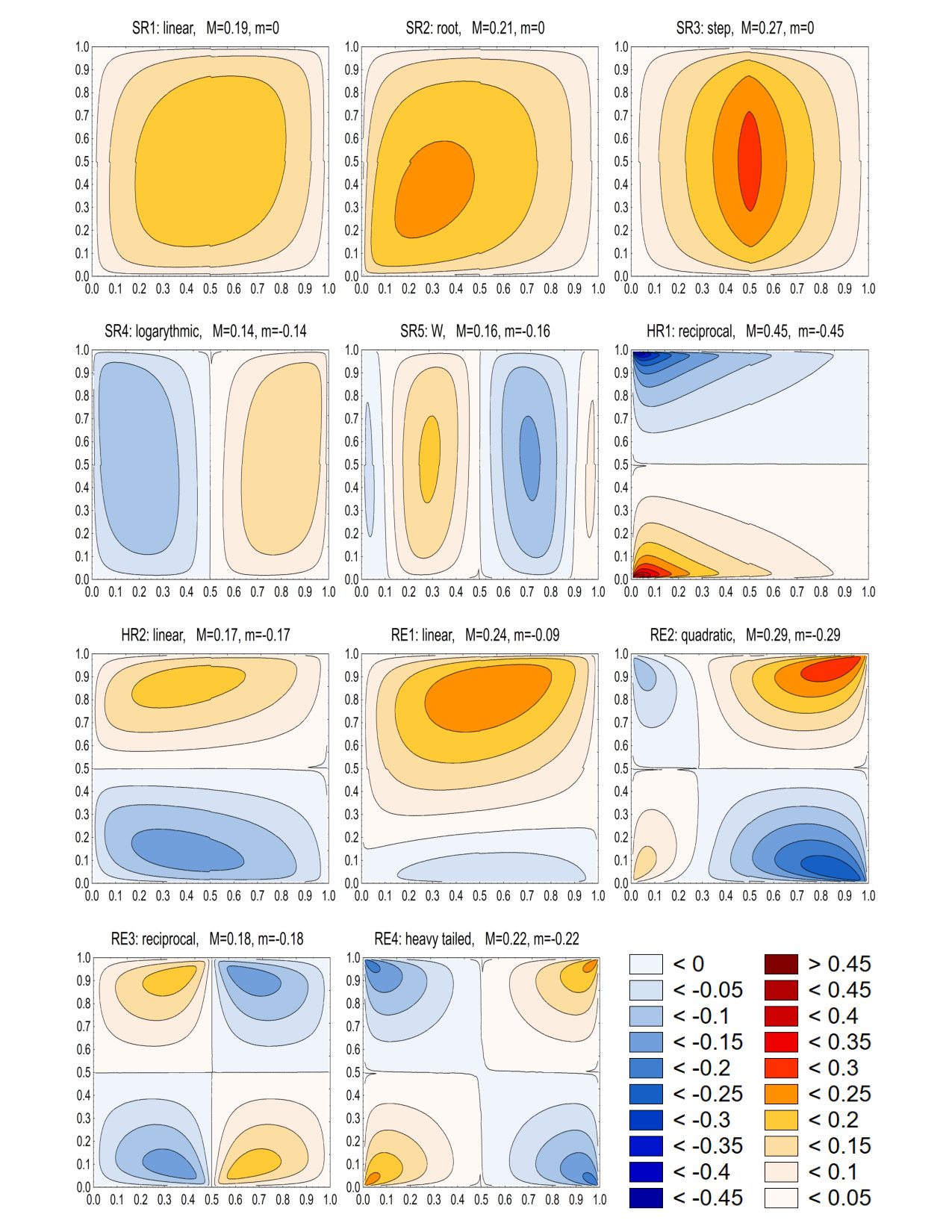 Figure 1
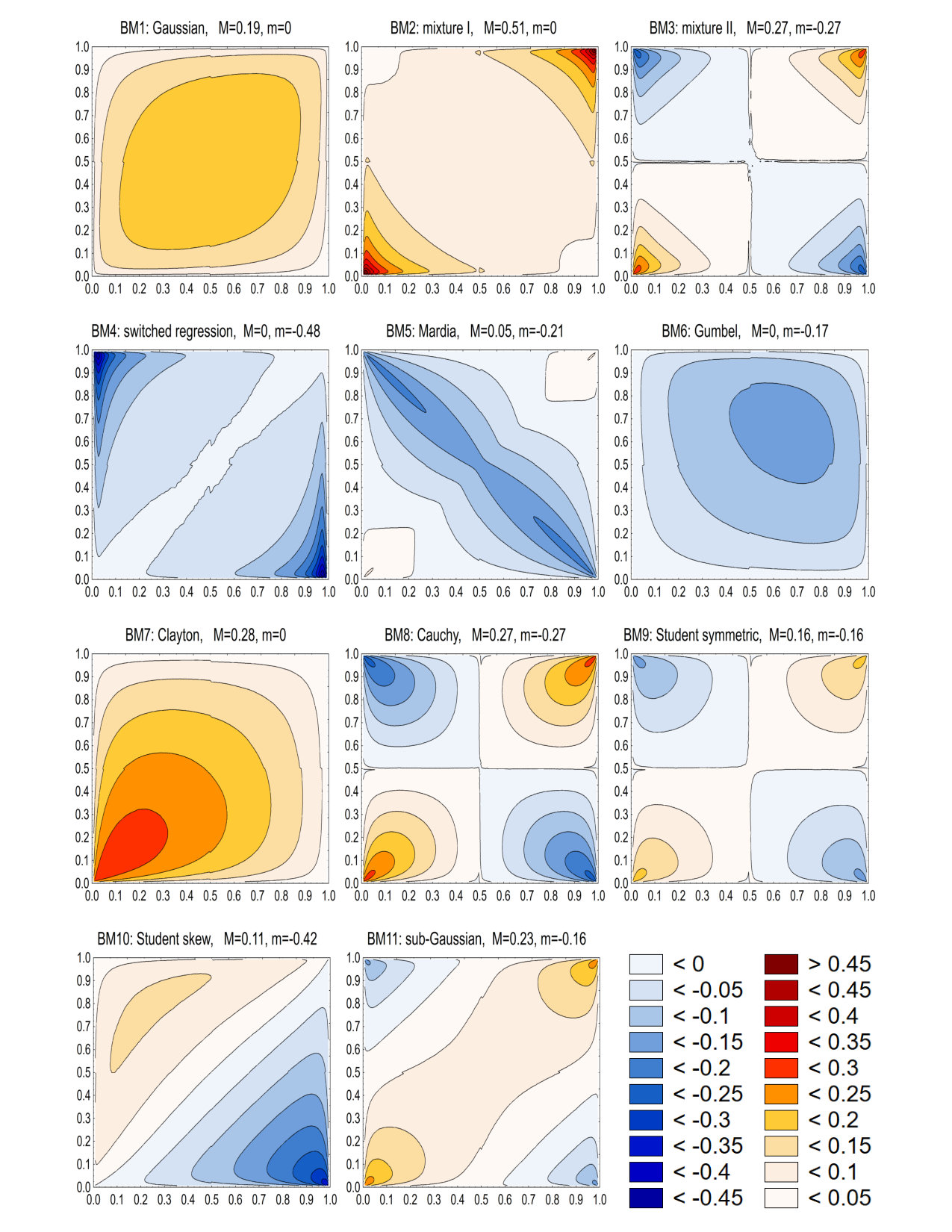 Figure 2
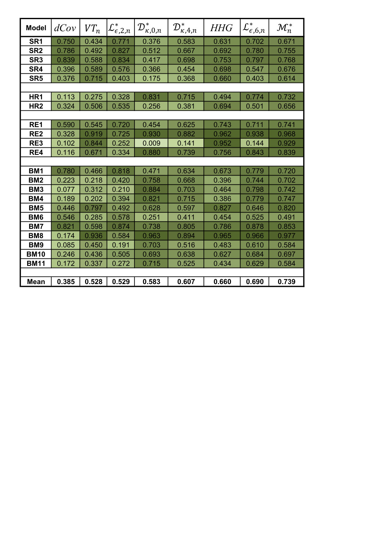 Figure 3
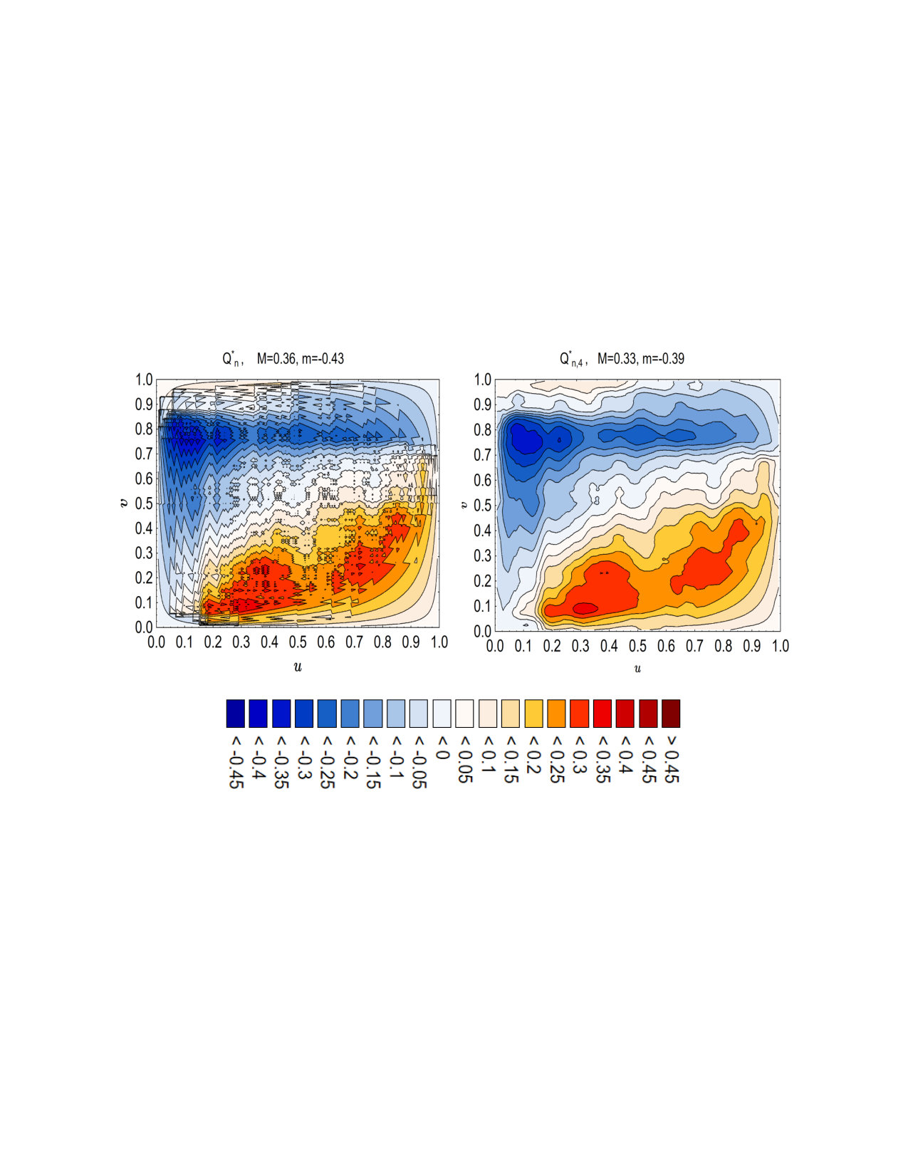 Figure 4
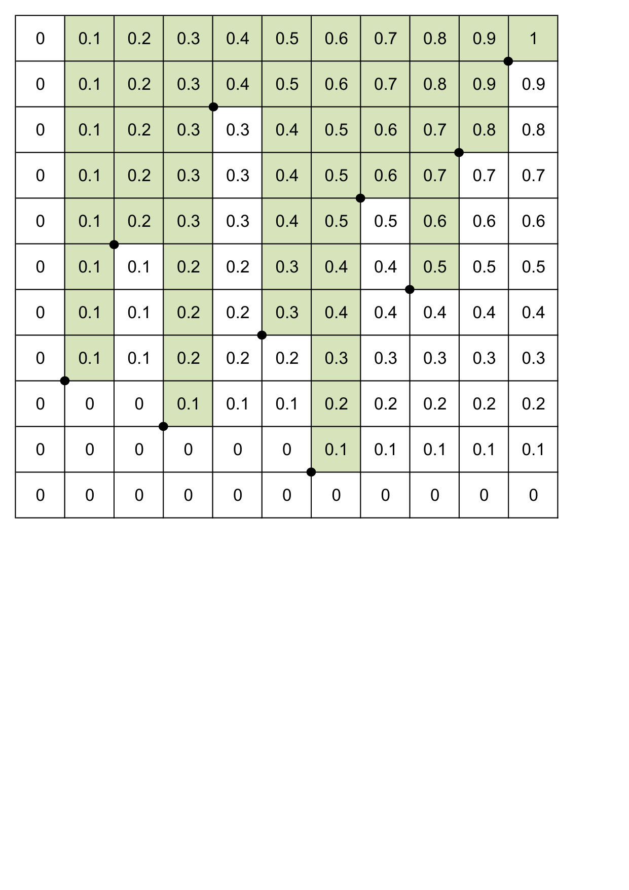 Figure 5
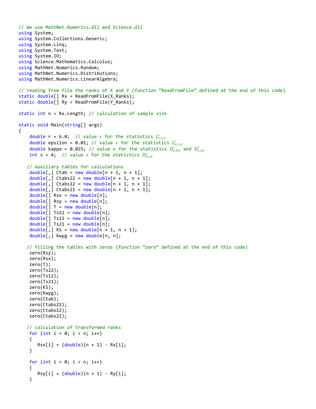 Figure 6
Peer Reviews
No public reviews on file for this paper yet. If you reviewed it on a platform where reviews are public (OpenReview, ICLR, NeurIPS, ICML), you can paste yours below so the community can read it here.
Videos
No videos yet. Explain this paper in a talk, walkthrough, or lecture? Add one.
Taxonomy
TopicsAdvanced Statistical Methods and Models · Financial Risk and Volatility Modeling · Statistical Methods and Inference
Validation of Association
Bogdan Ćmiel
Faculty of Applied Mathematics, AGH University of Science and Technology,
Al. Mickiewicza 30, 30-059 Cracov, Poland
e-mail: [email protected]
and
Teresa Ledwina
Institute of Mathematics, Polish Academy of Sciences
ul. Kopernika 18, 51-617 Wrocław, Poland
e-mail: [email protected]
Abstract
Recognizing, quantifying and visualizing associations between two variables is increasingly important. This paper investigates how a new function-valued measure of dependence, the quantile dependence function, can be used to construct tests for independence and to provide an easily interpretable diagnostic plot of existing departures from the null model. The dependence function is designed to detect general dependence structure between variables in quantiles of the joint distribution. It gives an insight into how the dependence structures changes in different parts of the joint distribution. We define new estimators of the dependence function, discuss some of their properties, and apply them to construct new tests of independence. Numerical evidence is given on the test’s benefits against three recognized independence tests introduced in the previous years. In real-data analysis, we illustrate the use of our tests and the graphical presentation of the underlying dependence structure.
Keywords: Copula; Cross-quantilogram; Independence testing; Measure of dependence; Quantile, Weighted statistics
1 Introduction
Measuring dependence and testing for independence have been intensively studied over the recent years. On the one hand, in many applied sciences it is a fundamental question how to quantify the dependence between variables under study. On the other hand, the present-day knowledge demonstrates that classical solutions are designed to capture specific, relatively simple, structures of dependence between two random variables. Thus they are not well suited to the scope of modern statistical analysis, and therefore may lead to completely misleading conclusions. Another inspiration is exploratory data analysis, where one of the goals is to investigate a large data set and search for pairs of variables which are closely associated. Obviously, the dependence structure of random vector cannot be neglected in reliable data analysis. In particular, this problem is crucial in insurance and finance. For example, Albers, (1999) showed that substantial deviations in the fair price of stop-loss premiums may occur even when there are small departures from independence. For further evidence and related discussion see Kass, (1993), Dhaene and Goovaerts, (1997), and Dhaene et al., (2009).
These challenges have stimulated great development in the area of evaluation of relationships, measuring their strength and testing for a lack of dependence via pertinent statistics. An emphasis has been put on capturing complex dependence structures which cannot be detected by classical solutions. For an illustration of several ideas and approaches to quantifying dependence and detecting associations which have been considered over the last decade (in chronological order), see: Székely and Rizzo, (2009), Delicado and Smrekar, (2009), Reshef et al., (2011), Póczos et al., (2012), Zheng et al., (2012), Heller et al., (2013), Kwitt and Neumeyer, (2013), Reimherr and Nicolae, (2013), Berentsen and Tjøstheim, (2014), Vexler et al., (2014), Ledwina, (2015), Heller et al., (2016), Reshef et al., (2016), Bagkavos and Patil, (2017), Ding et al., (2017), Xu et al., (2017), Vexler et al., (2017), Wang et al., (2017), Reshef et al., (2018), Vexler et al., (2018), Zhang et al., (2018). These papers also discuss many earlier ideas and developments. Most of them concern bivariate vectors and independent observations. A parallel stream of articles deals with dependent data and multivariate observations. It is beyond the scope of this paper to survey these more general situations.
The present paper proposes and studies new tests of independence which are closely related to the function-valued measure of dependence proposed in Ledwina, (2014, 2015). The measure is conceptually appealing and has a straightforward interpretation facilitating a comprehensive view of the association structure. The pertaining tests are of simple form and have good power. Their extension to multivariate observations, dependent data, and for detecting positive or negative dependence is straightforward. Additionally, their big advantage is a natural link to an easily interpretable diagnostic plot. Consequently, in the case of rejection of the hypothesis on independence, reliable information on which part of the population — and to which extent — invalidates the hypothesis is available.
In many practical situations variables are measured in different scales. Therefore, a common requirement is to consider dependence measures that are invariant to strictly increasing transformations of the marginal variables. The copula-based dependence measures fulfill the above postulate and therefore are scale invariant. Several real-valued measures of such type have been studied for a long time. For a nice overview see Schweizer and Wolf, (1981), and Ding and Li, (2015). However, nowadays there is strong evidence that attempting to express a complex dependence structure via a single number is hopeless. Vexler et al., (2017) admitted that such a conclusion was clearly spelled out as early as in the celebrated book by Kendall and Stuart, (1961).
To help understand the underlying dependence structure with aid of a procedure invariant under strictly increasing transformations of the marginal distributions, Fisher and Switzer, (1985) proposed a rank-based graphical tool called a chi-plot. The procedure is rather complicated and not easy to interpret. A simpler solution was introduced by Genest and Boies, (2003). Their display is called a Kendall plot and refers to the idea of a Q-Q plot. It also is based on ranks and is more directly related to the underlying copula function than the chi-plot. See also Vexler et al., (2018) for further development of this idea. Ledwina, (2014, 2015) has proposed a simple dependence measure which is explicitly based on the copula function. The measure aggregates some Fourier coefficients of the copula in some special non-orthogonal basis. Expansions in the Hilbert space using systems of functions which are not mutually orthogonal appear in the literature under the label “quasiorthogonal expansions”; cf. Daubechies et al., (1986). The above mentioned Fourier coefficients can also be interpreted in terms of some local correlations; cf. Ledwina and Wyłupek, (2014), p. 39, and Ledwina and Wyłupek, (2012), p. 361. For further interpretation see Remark 1, below. Here we mention only that the measure can be seen to be naturally related to the cross-quantilogram, a notion with growing importance in econometry.
The remainder of the article is organized as follows: Section 2 recalls the definition of the measure and its properties, shows some links of to other existing notions, and illustrates the shape of the measure in a series of interesting bivariate models considered in recent literature on independence testing. Section 3 introduces a new useful estimator of . In Section 4, we present three new test statistics pertaining to the proposed estimator of . Two test statistics are the supremum-norm and integral-norm of the estimated , respectively. The third solution exploits the minimum -value principle. We also report there basic theoretical results on the new tests. In Section 5, we provide a comparative study on power analysis for the new solutions and some competitors which have been already introduced in the literature on the subject. Section 6 contains a study of a real data example. Proofs of all results are relegated to Supplementary Materials, which are located at final part of the manuscript. In the Supplementary Materials we include also some comments on our implementation of new statistics, and provide related C codes.
2 A Copula-Based Measure of Dependence: the Quantile Dependence Function
2.1 Definition and Properties
Consider a pair of random variables and with bivariate cumulative distribution function and with continuous margins and , respectively. Then there exists a unique copula such that . Obviously, and , appearing in this formula, are the -quantile and -quantile of the respective marginal distribution functions. Set
[TABLE]
We shall call the quantile dependence function. By (1), the measure attributes the copula to the continuous function on . As stated and justified in Ledwina, (2014, 2015), the measure fulfills natural postulates, motivated by the axioms formulated in Schweizer and Wolf, (1981) and updated in Embrechts et al., (2002). For convenience, we recall here the basic properties of . Below, we set
[TABLE]
Proposition 1**.**
The quantile dependence function , given by (1), has the following properties.
* for all .* 2. 2.
By the Fréchet-Hoeffding bounds for copulas, the property 1 can be further sharpened to where and . 3. 3.
* is maximal (minimal) if and only if and is strictly increasing (decreasing) a.s. on the range of .* 4. 4.
* if and only if and are independent.* 5. 5.
The equation , a constant, can hold true if and only if . 6. 6.
* is non-negative (non-positive) if and only if are positively (negatively) quadrant-dependent.* 7. 7.
* is invariant under transformations which are strictly increasing a.s. on ranges of and , respectively.* 8. 8.
If and are transformed by strictly decreasing a.s. functions, then is transformed to . 9. 9.
If and are strictly decreasing a.s. on ranges of and , respectively, then ’s for the pairs and take the forms and , accordingly. 10. 10.
* respects concordance ordering, i.e. for cdf’s and with the same marginals and corresponding copulas and , for all implies for all .* 11. 11.
If and are pairs of random variables with joint cdf’s and , and the corresponding copulas and , respectively, then weak convergence of to implies for each .
Remark 1**.**
The measure can be explicitly related to some tail-dependence indices: lower tail-dependence coefficient and the coefficient of upper tail dependence , which are defined in the situations when the respective limits exist; coefficients of tail dependence: and . In particular, on the diagonal, while on anti-diagonal . See Sibuya, (1960), and Chicheportiche, (2013), respectively.
The measure is weak-equitable and weakly-robust-equitable in the sense of Definitions 2 and 4 in Ding et al., (2017), accordingly.
For radially symmetric copulas where it holds that , where stands for generalized Blomqvist’s measure of concordance considered in Schmid and Schmidt, (2007).
Finally note that coincides with the cross-quantilogram applied to . Therefore, using precise terminology, we can say that is the cross-correlation of the respective quantile hits. The cross-quantilogram for time series was, somewhat in passing, introduced on p. 261 in Linton and Whang, (2007) in the context of predictability studies. In Han et al., (2016) the idea has received considerable attention and development.
2.2 Graphical illustration
Given a formula for , the quantile dependence function can be graphically presented in many convenient ways. However, in the next section we introduce a new estimate of and here we simply display the corresponding (averaged) values of the estimate for large , and for several interesting forms of dependence of and . To be specific, in Figures 1 and 2 we took and calculated the averages over 10 000 MC runs. This gives quite precise information on the shape of .
To see how the measure reflects different forms of dependence and to study empirical powers of new tests proposed in Section 4, we have considered a wide spectrum of models. Some of them are classical ones, a considerable portion has been recently introduced in different simulation experiments in some related papers, a few of the models have been defined just for this study. Below we only show the sources of some recently introduced models. Classical ones were used in numerous earlier simulation studies. Throughout the paper stands for the indicator of the set . The list of models is as follows.
Simple Regression:
- SR1:
linear ; Vexler et al., (2014);
- SR2:
root ; Simon and Tibshirani, (2012), Reshef et al., (2018);
- SR3:
step ; Simon and Tibshirani, (2012), Reshef et al., (2018);
- SR4:
logarithmic ; Vexler et al., (2014);
- SR5:
W ; Ding and Li, (2015).
Heterosceadestic Regression:
- HR1:
reciprocal has exponential distribution with , ;
- HR2:
*linear * .
Random-Effect-Type Models:
- RE1:
linear , Vexler et al., (2014);
- RE2:
quadratic , Vexler et al., (2017);
- RE3:
reciprocal , Vexler et al., (2017);
- RE4:
heavy tailed is bivariate Cauchy. Define , , Supplemental Material for Vexler et al., (2017).
Bivariate Models:
- BM1:
Gaussian bivariate normal distribution with ;
- BM2:
mixture I the mixture (0.1)(standard bivariate Gaussian) + (0.9)(bivariate Gaussian with mean 0, variances 6 and the covariance 5);
- BM3:
mixture II the mixture (0.3)(bivariate Cauchy) + (0.7)(standard bivariate Gaussian);
- BM4:
switched regression for and otherwise;
- BM5:
*Mardia * Mardia family of copulas with ;
- BM6:
*Gumbel * Gumbel bivariate distribution with ;
- BM7:
Clayton Clayton model with ;
- BM8:
Cauchy bivariate Cauchy distribution;
- BM9:
Student symmetric symmetric Student’s distribution with 2 degrees of freedom;
- BM10:
Student skew skew bivariate Student’s distribution with 5 degrees of freedom and parameters ;
- BM11:
sub-Gaussian bivariate sub-Gaussian distribution with parameters , Kallenberg and Ledwina, (1999).
Each panel in Figures 1 and 2 only has a short label related to the above detailed description. Moreover, to increase readability, each label also contains two numbers and which are the maximal and minimal values, respectively, of the corresponding for .
3 Symmetrized estimate of
3.1 Motivation
Let be independent and identically distributed random vectors drawn from a bivariate distribution function with continuous marginals and . Furthermore, let denote the rank of in the sample , while stands for the rank of in the sample .
A natural way of estimating , given by (1), is the plug-in method. There are several estimators of available. The first proposal presumably goes back to Ruymgaart, (1973), see pp. 6 and 12, and has the form
[TABLE]
Monte Carlo simulations show that it is better to use
[TABLE]
Under the above assumptions, and differ by almost surely. Alternatively, one can include the continuity correction in . Another option are kernel based smooth versions of or ; cf. Fermanian et al., (2004), Omelka et al., (2009) and the references therein. A different smoothed variant has been proposed by Sancetta and Satchell, (2004). They introduced the Bernstein copula estimator, which has been further studied by Janssen et al., (2012), and Segers et al., (2017), among others.
It should be emphasized, however, that our ultimate goal is not the estimation of the copula itself, but a construction of some tests of independence based on the corresponding estimator of . In such an application, excessive smoothing of the underlying parameter, i.e. the copula function, is often not profitable to the power of the resulting test. On the other hand, we shall consider test statistics as functionals of the process , where is an estimate of the copula, while the weight is given by (2). Therefore, we have to be very careful about the behavior of the quantity near the edges of . In this sense, is not convenient for our purposes. It can be seen that the expression takes on very large (absolute) values near the points (0,1), (1,0) and (1,1). In contrast, empirical behavior of near (0,0) is satisfactory. Therefore, to estimate the numerator of , i.e. the function
[TABLE]
say, we propose and we shall apply a symmetrized variant of the random function
[TABLE]
which exploits the useful behavior of in the first quadrant.
3.2 Symmetrization
To define the symmetrization, note that the numerator of , for every , can be rewritten in the following four forms
[TABLE]
Therefore, similarly as in (3), we can consider the following variants of estimators of .
[TABLE]
This leads us to the symmetrized estimator of given by
[TABLE]
Note that for any it holds that
[TABLE]
We shall call the symmetrized version of the process . Finally, the initial and symmetrized estimators of are given by
[TABLE]
respectively. Note that outside the estimator is deterministic, bounded, and it tends to 0 when its arguments approach the edges of . This makes a great difference in finite sample behavior in comparison with , given in (6) as well.
We shall also consider a smoothed variant of . To be specific, for some we shall use
[TABLE]
The three above defined estimators of have the following useful property:
Proposition 2**.**
Let be independent and identically distributed random vectors drawn from a bivariate population obeying a joint distribution function with continuous marginals and . Under the independence of and , given , it holds that
[TABLE]
where stands for convergence in distribution.
This, in particular, makes it possible to immediately see on the graphs of the estimates of some evidence indicating in which part of the population and to which extent (at least roughly) the independence is invalidated. Formal tests, based on some functionals of these estimators, are defined in Section 4.
4 New weighted test statistics and their properties
For continuous random variables, testing for independence is equivalent to verification if the true copula is equal to the independence copula. Therefore, we consider the null hypothesis of the form
[TABLE]
and study test statistics defined as some functionals of the estimated difference .
4.1 Integral statistics
Weighted integral copula-based statistics of the form
[TABLE]
where and , were studied in Deheuvels et al., (2006). Recently, Berghaus and Segers, (2018) have introduced the independence statistic which in the two dimensional case reads as
[TABLE]
where is the empirical beta copula - a particular case of the empirical Bernstein copula, , and .
We shall consider the (standardized) -norm of
[TABLE]
In view of the form of , cf. (6), is a weighted integral-type statistic for the symmetrized version of the process , where the weight is given by (2). For relatively small one could find a closed expression for . In general, for reasonably large values of , it suffices to approximate the value of by \frac{\sqrt{n}}{(n+1)^{2}}\bigl{\{}\sum_{i=1}^{n}\sum_{j=1}^{n}\big{|}Q_{n}^{*}(\frac{i+0.5}{n+1},\frac{j+0.5}{n+1})\big{|}^{r}\bigr{\}}^{1/r}.
To achieve consistency of statistics like (9), using some existing results on the classical empirical copula process, we have to slightly modify the integration area in (9) around the vertices of . For an illustration, given , we shall consider
[TABLE]
and the modified variant of given by
[TABLE]
To derive the consistency of , some smoothness assumptions have to be imposed on the underlying copula . The following non-restrictive requirements have been formulated in Segers, (2012) and turn out to be sufficient in many practically important situations. For more details, see Segers, (2012), and Berghaus and Segers, (2018).
Assumption 0**.**
and exist and are continuous on and , respectively; 2. 2.
exists and is continuous on ; 3. 3.
There exists a constant such that \;\;\Bigl{|}\frac{{\partial}^{2}}{\partial u\partial v}C(u,v)\Bigr{|}\leq K\min\Bigl{\{}\frac{1}{u(1-u)},\frac{1}{v(1-v)}\Bigr{\}},\; for .
Proposition 3**.**
Assume that the underlying copula satisfies the Assumption ‣ 4.1. Consider any and a positive . Suppose that in such a way that , as . Then, under the alternative corresponding to , the test rejecting for large values of is consistent.
4.2 Minimum -value statistics
A test rejecting for large values of the distance is expected to be especially sensitive to alternatives shifting the probability mass towards the edges of . In contrast, the statistic proposed in Heller et al., (2013) proves to be very efficient in detecting some noisy functional relationships. Therefore, it seems useful to propose a procedure which combines advantages of both solutions. Our approach to this question is via combining -values. For this purpose denote by the rank variant of the statistic, based on pairwise distances, introduced in Heller et al., (2013). Given the sample , let denote -value of and let be respective -value of .
We propose to reject for small values of
[TABLE]
The idea of a minimum -value statistic goes back to Tippett Tippett, (1931).
4.3 Supremum-type solutions
Another classical approach to measuring departures from is by taking a supremum norm of . More precisely, given one can consider
[TABLE]
Analogously to , can be interpreted as weighted sup-type statistic. However, extensive simulations, which shall be partially reported in Section 5, have shown that it is not necessarily a very powerful solution and some smoothing of improves the finite sample behavior of such constructions. Therefore, we shall take into account and introduce the corresponding class of supremum type statistics
[TABLE]
Obviously, with coincides with the solution (12). Supremum type statistics are particularly convenient for interpretation of obtained values of the selected estimator of the measure and at least rough, but practically immediate, evaluation of the extent to which is possibly invalidated.
Proposition 4**.**
Suppose that the requirement 1. of Assumption ‣ 4.1 holds for . Consider positive such that and , as Then, tests rejecting for large values of and , respectively, are consistent under the alternative .
5 Simulated powers
We shall study the empirical behavior of the following statistics:
- •
the statistic rank-dCov of Székely and Rizzo, (2009), Section 4.3. We shall concisely denote this variant by , as done in Heller et al., (2016), p. 17, as well;
- •
the rank based variant of the statistic introduced in Heller et al., (2013), denoted by HHG, similarly as proposed in Heller et al., (2016), p. 17;
- •
the empirical likelihood ratio test , defined on p. 160 of Vexler et al., (2014);
- •
for two choices of and ;
- •
for two values of and ; as usual in this area, the supremum in the Kolmogorov-Smirnov statistic was replaced by a maximum over a grid of points.
- •
using HHG and with .
The outcomes of our Monte Carlo experiments, done for and the significance level , are collected in Table 1. Table 1 presents empirical powers under the 22 models introduced in Section 2.
The simulation results show that with outperforms (in the average) the rank distance covariance and also slightly the empirical likelihood ratio test. The rank based statistic HHG is slightly more powerful (in the average) than while our second solution with provides some improvement over the two last mentioned statistics. The most powerful solution turns out to be our third, , which combines the advantages of HHG (high power for regression models) with the benefits of (sensitivity to heavy tails). It is also worth noting that turns out to be much less sensitive to the choice of than . In particular, under our simulation scheme, for works much worse than its smoothed version .
In view of the simulation results it appears that the class of statistics shows considerable potential for further use. On the one hand, the integration process naturally smooths , and extra smoothing seems to be unnecessary. We have also investigated some smoother integrands in -type norm statistics, but they have not resulted in more stable powers, and no average gain of power has been noticed. So, this is one advantage of such a solution over the supremum-type ones. On the other hand, it is well known that the -norm, under , approximates the supremum norm. Therefore, the class is flexible and enough reach. Needless to say, such smooth functionals of weighted empirical processes are also easier to analyze than weighted supremum-type statistics. Obviously, several questions arise in the context. The first one is the choice of . In the course of the present simulation study we have simply inspected and decided for . However, it is possible to study the problem more deeply and carefully, by calculating for example asymptotic relative efficiency of with respect to some standard, and investigating the classes of alternatives for which particular recommendations about are optimal. A recent paper by Inglot et al., (2018) provides tools that make it possible to answer to such a question. Obviously, solving such a problem is a fairly non-trivial task.
Finally, note that the test statistic performs very well. It has relatively simple structure which nicely reflects the advantages of its ingredients. The solution is similar in spirit to a much more complex one proposed in Heller et al., (2016). The latter combines -values of chi-square-type tests over increasingly fine data-dependent sample space partitions.
6 Application
We demonstrate our testing procedures on a data set of aircraft span (X) and speed (Y) data, on log scales, from years 1956-1984, collected by Saviotti, and reported and studied in Bowman and Azzalini, (1997). Standard empirical correlation measures, such as Pearson’s, Spearman’s, and Blomqvist’s rank statistics, applied to this data, do not invalidate independence, as their -values are well above 0.7. This suggests that any dependence structure, if present at all, is likely to be nonlinear. Székely and Rizzo, (2009), and Heller et al., (2013) have applied their tests to this data and have received very small -values (less than 0.00001). In conclusion, the above evidence implies strong nonlinear dependence structure.
This data was also analyzed by Jones and Koch, (2003), and Berentsen and Tjøstheim, (2014). The two papers contain a presentation of some empirical dependence measures, defined on . Jones and Koch, (2003) have started with a local dependence function of Holland and Wang, (1987) and proposed a so-called dependence map. The result of this approach suggests a rather complicated picture of the joint behavior of and ; cf. their Figure 2. In turn, Berentsen and Tjøstheim, (2014) have applied another local correlation concept, namely the local Gaussian correlation introduced in Tjøstheim and Hufthammer, (2013). The approaches by Jones and Koch, (2003), and Berentsen and Tjøstheim, (2014), are related to estimation and modeling bivariate densities on , respectively. The second solution is especially technically involved. The overall picture resulting from both implementations is very similar; cf. Figure 4 in Berentsen and Tjøstheim, (2014): on the plane there are three separated regions in which local dependence is positive, one region in which it is negative. There are also areas on the plane with no local dependence between log(span) and log(speed).
In Figure 3 we show two our estimators and for these data. The quantile dependence function , relying on the copula, separates the dependence structure from any marginal effects. At first glance it can be noticed that the dependence pattern, which has been revealed by the estimated , is much simpler than the above mentioned pictures suggest. Both our displays show two separated regions of strong dependence (positive and negative) of spans and speeds. Spans in the range from the second to ninth decile are positively correlated with speeds lying below their median. For speed above the median and below the ninth decile, a strong negative trend is exhibited. There is also a large region of -quantiles and -quantiles in which the variables span and speed seem to be unrelated.
It is visible at first glance that in some regions of points ’s of the right hand panel in Figure 3 the absolute value of exceeds values which, in view of Proposition 2, are highly improbable under the null hypothesis. For instance, Arguing formally, all -values of our new statistics , , and related are practically 0.
7 Conclusion
In this article, we proposed a framework for measuring and visualizing the dependence structure, and constructing formal tests of independence of two random variables. Our approach exploits the quantile dependence function , a recently introduced local dependence measure. The function gives a detailed picture of the underlying dependence structure. It provides a means to carefully examine local association structure at different quantile levels. The measure distinguishes between negative and positive quadrant dependence and can be immediately generalized to the multivariate case. We have proposed three new tests based on simple and useful nonparametric estimators of the measure. Estimating the measure naturally leads to some weighted copula processes. Our test statistics are based on classical supremum-type and integral-type functionals of the related processes. Both the measure and the corresponding test statistics are invariant under strictly increasing transformations of observations. These statistics are easy and fast to calculate. A more refined solution has been proposed as well. Some consistency results are stated and proved, and extensive evidence on stability of empirical powers of new solutions is provided. Finally, we have applied our approach to analyze Saviotti aircraft data. This application shows the usefulness of the proposed inference tools in two respects: as a simple and reliable graphical device allowing for visual inspection of regions of evident departures from independence and formal tests verifying validity of the independence structure.
8 Supplementary Materials
**Appendix A: Proofs
**
**A.1 Proof of Proposition 2
**
The first part of (8) follows immediately from Theorem 3 in Fermanian et al. (2004) and the forms of the limiting process and pertaining covariance.
To prove the second statement of (8) let us introduce auxiliary rank process and recall the abbreviated notation for our weight function
[TABLE]
where is given by (3). With these notation we have: for each fixed it holds that . Hence , provided that is true. The last statement is key observation to complete a proof of the second part of (8). Indeed, consider the succeeding expression appearing in , which in turn defines . We have
[TABLE]
while denotes the integer part of the number . Analogously,
[TABLE]
and
[TABLE]
Obviously, the relations (A.2)-(A.4) hold irrespective of is true or not. Under , asymptotic normality of and the above yield the required statement for .
Now we shall show that and are close enough to infer the last statement in (8) from the middle one. For this purpose take any . We claim that for it holds that: there exists and a constant such that for all
[TABLE]
Without loss of generality assume that . Set
[TABLE]
Then, there exists such that Moreover, for any it holds that . Hence, for any
[TABLE]
[TABLE]
[TABLE]
Since is continuous and bounded on , therefore there exists such that for all
[TABLE]
By (A.6) and (A.7),
[TABLE]
[TABLE]
This proves (A.5) and finally yields the last conclusion in (8).
In view of (5) and an analogous relations for , the zero set of the denominator in (6) is included in the zero set of the numerators in (6). Hence, we can additionally define and on this set to be 0. With this convention, the sample paths of and are bounded on . This enables to treat and as random elements with values in . This observation helps us to use below some ready results on weighted copula process.
A.2 Proof of Proposition 3
We shall consider the integral on four subsets of in (10), separately. On the set it holds that , where is defined in (A.1). On the set we have
[TABLE]
[TABLE]
[TABLE]
Moreover, the process \sqrt{n}\Bigl{\{}\frac{1}{n}\sum_{i=1}^{n}{\bf 1}\Bigl{(}\frac{R_{i}}{n+1}>1-s,\frac{S_{i}}{n+1}>1-t\Bigr{)}-st\Bigr{\}} has the same distribution as the process , where is the rank process for the sample , where the functions and are strictly decreasing. It is so because the ranks of the transformed observations and , say, are related to and as follows . For the two remaining subsets of the integration area similar argument applies. It shows that asymptotic behavior of is determined via pertaining asymptotics of the variables
[TABLE]
Moreover,
[TABLE]
On the other hand, under the Assumption 0, by Theorem 2.2 of Berghaus et al. (2017), the empirical copula process
[TABLE]
for is well approximated, in some weighted supremum norm, by pertaining bivariate empirical process . To define set , and
[TABLE]
Next, introduce the (unobservable) empirical process , based on ,
[TABLE]
and finally define
[TABLE]
where and . With this notation,
[TABLE]
where and . Moreover, it holds that converges weakly in , equipped with the supremum norm, to centered Gaussian process.
The above implies that asymptotic behavior of the linear functional is determined by respective asymptotics of the weighted bivariate empirical process and its pertaining variants, provided that we are well controlling the magnitude of . Note also that asymptotic behavior of
[TABLE]
is decisive to the asymptotic power of under the alternative pertaining to . By symmetries of and , we have
[TABLE]
In the last integral the behavior of is crucial. Hence, the requirement follows. This implies our assumption
The above yields
[TABLE]
where and are absolute constants. Hence, under our assumptions on , . The above implies that asymptotics of , under , is determined by the two terms: a random component, which is at most and an asymptotic shift, which is at least . This ensures the consistency.
A.3 Proof of Proposition 4
Due to 1. of the Assumption 0, by Proposition 3.1 of Segers (2012), the process , given in the equation (A.8), converges weakly in to the Gaussian process , defined by (3.1) in Segers (2012). This implies that for any , as ,
[TABLE]
On the other hand, by (6),
[TABLE]
Under the alternative , the second term in (A.13) is, in , at least . Therefore, the assertion (A.12) along with the assumptions on yield the consistency of .
The case of can be treated similarly, as by (A.2)-(A.4), in an analogue of (A.13) an immaterial extra term, being at most , appears, only. Hence, for ’s under consideration, the consistency of follows.
To prove consistency of the test rejecting for large values of observe that always it holds that . Let be a critical value of -level test based on . By the above, . On the other hand, by (A.5), under any alternative defined by the underlying ,
[TABLE]
In view of the proof of the consistency of the smoothed variant is concluded.
References
- (1) Berghaus, B., Bücher, A., Volgushev, S. (2017). Weak convergence of the empirical copula process with respect to weighted metrics. Bernoulli 23, 743-772.
- (2) Fermanian, J.-D., Radulović, D., Wegkamp, M. (2004). Weak convergence of empirical copula processes. Bernoulli 10, 847-860.
- (3) Segers, J. (2012). Asymptotics of empirical copula processes under non-restrictive smoothness assumptions. Bernoulli 18, 764-782.
**Appendix B: Data set referenced in the article
**
Aircraft span and speed data, from the third period, 1956-1984, are available in electronic form from A.W. Bowman and A. Azzalini (2007). R package ‘sm’: Nonparametric smoothing methods (version 2.2); https://cran.r-project.org/web/packages/sm/sm.pdf
**Appendix C: Description and Codes
**
In this Section we provide some codes for computation of , , , and comment on calculation of . We start with a preliminary information.
**C.1. Preliminaries
**
**Calculation of
**
Let us denote by and the vectors of ranks related to and , respectively. Set and , . Next, introduce the notation and for vectors of transformed ranks. Additionally define and . Recall also that, using and , we consider empirical copula of the form
[TABLE]
With these notations, the functions , appearing in the definition of , and hence in the formula (6) for , have the following alternative forms
[TABLE]
[TABLE]
[TABLE]
[TABLE]
for any . That is why we calculate the transformed ranks in our computer program and we calculate empirical copula for ranks and transformed ranks. Tables ”Ctab”, ”Ctabs12”, ”Ctabs22”, ”Ctabs21” contain values of the empirical copulas , , , , corresponding to a grid of points ’s, where
[TABLE]
Notice that a calculation of , on the grid , , , using the initial formula (C.1) is completely ineffective since for every point from the grid we have to calculate a sum of indicators. The computational complexity of that approach is . Much better method is the following recursion. If we sort vectors in ascending order according to the first coordinate, we obtain vectors , where is the rank in the vector corresponding to the rank in the vector . Observe that for all we have . Moreover, for all , and for it holds that
[TABLE]
Let us explain this recursion using the following example, in which we took . The resulting ’s were as follows: 3, 6, 2, 9, 4, 1, 7, 5, 8, 10. The entries of the presented table are equal to respective values of for , . It is useful to imagine that succeeding vertical and horizontal lines of the table are located at points
All entries in the first column are equal to [math]. In next columns the values on white background are equal to the first value on the left and the values on green background are equal to the first value on the left plus . When looking from the left to the right, black dots in the table are the sorted pseudo-observations . The computational complexity of that approach is . Tables ”T”, ”Ts12”, ”Ts22”, ”Ts21” contain second coordinates of the sorted vectors , , , , according to the first coordinate, respectively. Using the above recursion, we use them to calculate , , , on the grid , , . In view of (C.2), this allows to calculate on the grid. Pertaining values are collected by our program in a table ”KS”.
Calculation of and
We calculate
[TABLE]
on the grid , , numerically, i.e. we apply the approximation
[TABLE]
The values for , are collected in a table ”KWyg”.
Notice also that . So, in this way, both estimators of the quantile dependence function can be calculated.
**Calculation of
**
Using the definition of , given by the formula (10) of the paper, set
[TABLE]
We calculate numerically, i.e. we approximate
[TABLE]
In the computer code the approximate value of is denoted by ”I”.
**Calculation of ** and
Let us denote
[TABLE]
We calculate and numerically, i.e.
[TABLE]
In the computer code the approximate values of and are denoted by ”D0” and ”Ds”, respectively.
**Calculation of
**
A scheme of our program in this case was as follows. Given observations , we calculated pertaining values of statistics, L = and H = HHG, say, where HHG denotes rank based variant of test introduced in Heller et al. (2013). Note that basic part of a C code for the statistic HHG is given in Section 2 of Supplementary Material for this paper.
To estimate -values of both ingredients of we have applied Monte Carlo method. Namely, we have generated MC = 100 000 auxiliary samples of size from uniform distribution on and calculated for them respective values of both statistics. Next, we sorted values of in ascending order obtaining . Similarly, we obtained sorted values of HHG. Empirical -values for the obtained values and were estimated as follows
[TABLE]
Finally, we calculated .
References
- (1) Heller, R., Heller, Y., Gorfine, M. (2013). A consistent multivariate test of association based on ranks of distances. Biometrika 100, 503-510.
- (2)
**C.2. Codes
**
Below we give codes for computation of , , .
See pages - of program.pdf
The reference list from the paper itself. Each links out to its DOI / PubMed record.
- 1Albers, (1999) Albers, W. (1999). Stop-loss premiums under dependence. Insurance: Mathematics and Economics , 24:173–185.
- 2Bagkavos and Patil, (2017) Bagkavos, D. and Patil, P. N. (2017). A new test of independence for bivariate observations. Journal of Multivariate Analysis , 160:117–133.
- 3Berentsen and Tjøstheim, (2014) Berentsen, D. and Tjøstheim, D. (2014). Recognizing and visualizing departures from independence in bivariate data using Gaussian correlation. Statistics and Computing , 24:785–801.
- 4Berghaus and Segers, (2018) Berghaus, B. and Segers, J. (2018). Weak convergence of the weighted empirical beta copula process. Journal of Multivariate Analysis , 166:266–281.
- 5Bowman and Azzalini, (1997) Bowman, A. and Azzalini, A. (1997). Applied Smoothing Techniques for Data Analysis: The Kernel Approach with S-Plus Illustration . Oxford Science Publications, Clarendon Press, Oxford.
- 6Chicheportiche, (2013) Chicheportiche, R. (2013). Non-linear dependence in finance. These, Ecole Centrale des Arts et Manufactures. ar Xiv:1309.5073 .
- 7Daubechies et al., (1986) Daubechies, I., Grossman, A., and Meyer, Y. (1986). Painless nonorthogonal expansions. Journal of Mathematical Physics , 27:1271–1283.
- 8Deheuvels et al., (2006) Deheuvels, P., Peccati, G., and Yor, M. (2006). On quadratic functionals of the Brownian sheet and related processes. Stochastic Processes and their Applications , 116:493–538.