Graph-Embedded Multi-layer Kernel Extreme Learning Machine for One-class Classification or (Graph-Embedded Multi-layer Kernel Ridge Regression for One-class Classification)
Chandan Gautam, Aruna Tiwari, M. Tanveer

TL;DR
This paper introduces a novel multi-layer graph-embedded kernel ridge regression auto-encoder architecture for one-class classification, effectively detecting outliers using only normal samples, and demonstrates its superiority over existing methods on multiple datasets.
Contribution
It proposes a multi-layer graph-embedded kernel ridge regression auto-encoder framework for OCC, integrating local and global variance-based graph embeddings, and provides four variants outperforming state-of-the-art methods.
Findings
Four variants outperform existing OCC classifiers
Statistical significance confirmed by Friedman test
Effective on 21 benchmark datasets
Abstract
A brain can detect outlier just by using only normal samples. Similarly, one-class classification (OCC) also uses only normal samples to train the model and trained model can be used for outlier detection. In this paper, a multi-layer architecture for OCC is proposed by stacking various Graph-Embedded Kernel Ridge Regression (KRR) based Auto-Encoders in a hierarchical fashion. These Auto-Encoders are formulated under two types of Graph-Embedding, namely, local and global variance-based embedding. This Graph-Embedding explores the relationship between samples and multi-layers of Auto-Encoder project the input features into new feature space. The last layer of this proposed architecture is Graph-Embedded regression-based one-class classifier. The Auto-Encoders use an unsupervised approach of learning and the final layer uses semi-supervised (trained by only positive samples and obtained…
Click any figure to enlarge with its caption.
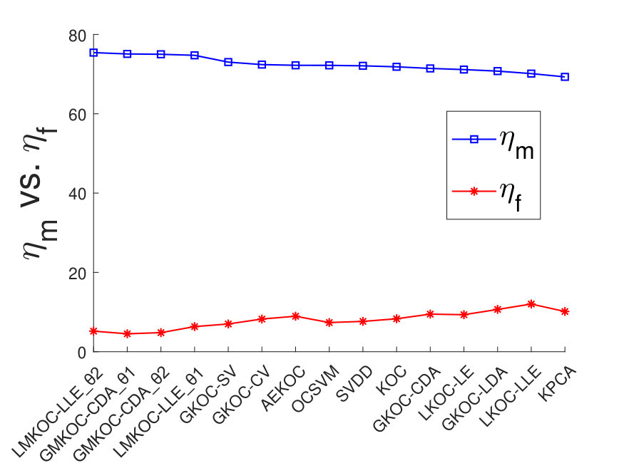 Figure 1
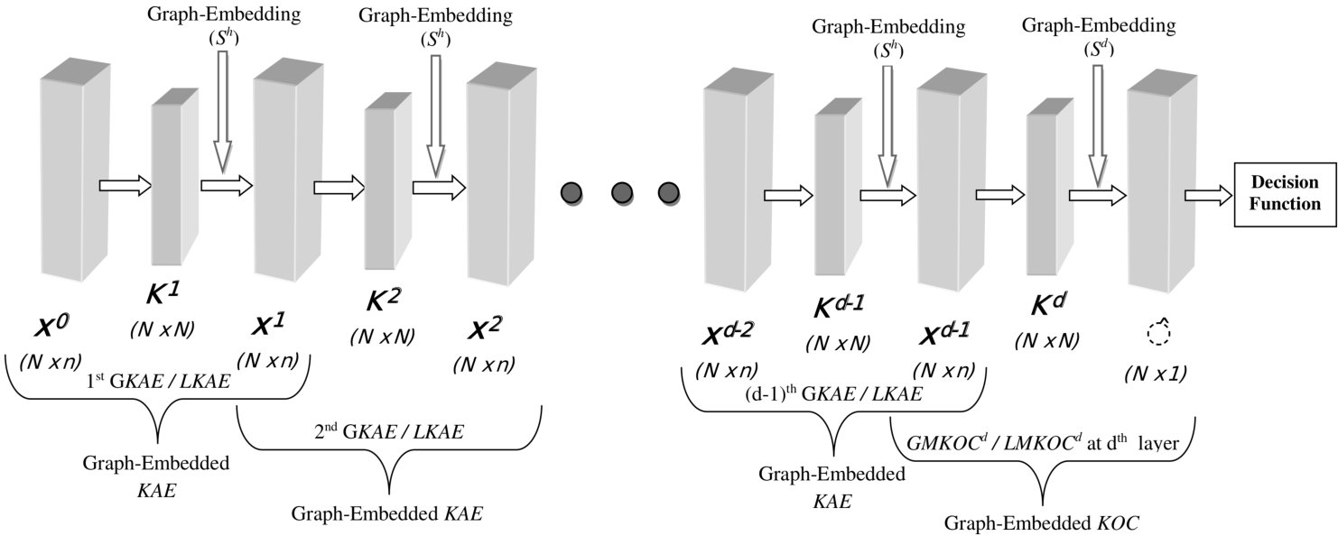 Figure 2
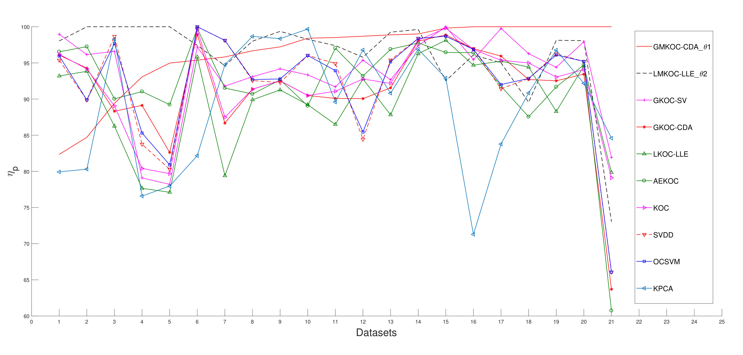 Figure 3
| S. No. | Name | #Targets | #Outliers | #Features | #samples \bigstrut |
| Financial Credit Approval Datasets \bigstrut | |||||
| 1 | Australia(1) | 307 | 383 | 14 | 690 \bigstrut[t] |
| 2 | Australia(2) | 383 | 307 | 14 | 690 \bigstrut[b] |
| 3 | German(1) | 700 | 300 | 24 | 1000 \bigstrut[t] |
| 4 | German(2) | 300 | 700 | 24 | 1000 \bigstrut[b] |
| 5 | Japan(1) | 294 | 357 | 15 | 651 \bigstrut[t] |
| 6 | Japan(2) | 357 | 294 | 15 | 651 \bigstrut[b] |
| Medical Disease Datasets \bigstrut | |||||
| 7 | Bupa(1) | 145 | 200 | 6 | 345 \bigstrut[t] |
| 8 | Bupa(2) | 200 | 145 | 6 | 345 \bigstrut[b] |
| 9 | Ecoli(1) | 143 | 193 | 7 | 336 \bigstrut[t] |
| 10 | Ecoli(2) | 193 | 143 | 7 | 336 \bigstrut[b] |
| 11 | Heart(1) | 160 | 137 | 13 | 297 \bigstrut[t] |
| 12 | Heart(2) | 137 | 160 | 13 | 297 \bigstrut[b] |
| 13 | Pima(1) | 500 | 268 | 8 | 768 \bigstrut[t] |
| 14 | Pima(2) | 268 | 500 | 8 | 768 \bigstrut[b] |
| Miscellaneous Datasets \bigstrut | |||||
| 15 | Glass(1) | 76 | 138 | 9 | 214 \bigstrut[t] |
| 16 | Glass(2) | 138 | 76 | 9 | 214 \bigstrut[b] |
| 17 | Iono(1) | 225 | 126 | 34 | 351 \bigstrut[t] |
| 18 | Iono(2) | 126 | 225 | 34 | 351 \bigstrut[b] |
| 19 | Iris(1) | 50 | 100 | 4 | 150 \bigstrut[t] |
| 20 | Iris(2) | 50 | 100 | 4 | 150 |
| 21 | Iris(3) | 50 | 100 | 4 | 150 \bigstrut[b] |
| One-class Classifier | (%) \bigstrut | |
|---|---|---|
| GMKOC-CDA_1 | 4.52 | 75.10 \bigstrut[t] |
| GMKOC-CDA_2 | 4.81 | 75.01 |
| LMKOC-LLE_2 | 5.19 | 75.43 |
| LMKOC-LLE_1 | 6.33 | 74.75 |
| \bigstrut[t] GKOC-SV | 7.00 | 73.04 |
| OCSVM | 7.36 | 72.22 |
| SVDD | 7.64 | 72.10 |
| GKOC-CV | 8.24 | 72.41 |
| KOC | 8.31 | 71.85 |
| AEKOC | 8.95 | 72.23 |
| LKOC-LE | 9.33 | 71.16 |
| GKOC-CDA | 9.48 | 71.44 |
| KPCA | 10.14 | 69.31 |
| GKOC-LDA | 10.67 | 70.77 |
| LKOC-LLE | 12.02 | 70.14 \bigstrut[b] |
| One-class Classifiers | (%) \bigstrut |
|---|---|
| GMKOC-CDA_1 | 96.33 \bigstrut[t] |
| LMKOC-LLE_2 | 96.20 |
| GMKOC-CDA_2 | 96.02 |
| LMKOC-LLE_1 | 95.44 |
| \bigstrut[t] GKOC-SV | 93.41 |
| GKOC-CV | 92.82 |
| OCSVM | 92.38 |
| SVDD | 92.27 |
| AEKOC | 92.00 |
| KOC | 91.83 |
| GKOC-CDA | 91.16 |
| LKOC-LE | 90.86 |
| GKOC-LDA | 90.33 |
| LKOC-LLE | 89.63 |
| KPCA | 89.20 \bigstrut[b] |
Peer Reviews
No public reviews on file for this paper yet. If you reviewed it on a platform where reviews are public (OpenReview, ICLR, NeurIPS, ICML), you can paste yours below so the community can read it here.
Videos
No videos yet. Explain this paper in a talk, walkthrough, or lecture? Add one.
Taxonomy
TopicsDomain Adaptation and Few-Shot Learning · Machine Learning and ELM · Anomaly Detection Techniques and Applications
\WarningFilter
captionUnsupported document class
11institutetext: C. Gautam 22institutetext: Indian Institute of Technology Indore, India
22email: [email protected] 33institutetext: A. Tiwari 44institutetext: Indian Institute of Technology Indore, India
44email: [email protected] 55institutetext: M. Tanveer 66institutetext: Indian Institute of Technology Indore, India
66email: [email protected]
Graph-Embedded Multi-layer Kernel Extreme Learning Machine for One-class Classification
or
Graph-Embedded Multi-layer Kernel Ridge Regression for One-class Classification
or
Graph-Embedded Multi-layer Least Square SVM with zero bias for One-class Classification
Chandan Gautam
Aruna Tiwari
M. Tanveer
Abstract
Introduction: A brain can detect outlier just by using only normal samples. Similarly, one-class classification () also uses only normal samples to train the model and trained model can be used for outlier detection.
Proposed Method: In this paper, a multi-layer architecture for is proposed by stacking various Graph-Embedded Kernel Ridge Regression () based Auto-Encoders in a hierarchical fashion. These Auto-Encoders are formulated under two types of Graph-Embedding, namely, local and global variance-based embedding. This Graph-Embedding explores the relationship between samples and multi-layers of Auto-Encoder project the input features into new feature space. The last layer of this proposed architecture is Graph-Embedded regression-based one-class classifier. The Auto-Encoders use an unsupervised approach of learning and the final layer uses semi-supervised (trained by only positive samples and obtained closed-form solution) approach to learning.
Experimental Results: The proposed method is experimentally evaluated on publicly available benchmark datasets. Experimental results verify the effectiveness of the proposed one-class classifiers over existing state-of-the-art kernel-based one-class classifiers. Friedman test is also performed to verify the statistical significance of the claim of the superiority of the proposed one-class classifiers over the existing state-of-the-art methods.
Conclusion: By using two types of Graph-Embedding, variants of Graph-Embedded multi-layer -based one-class classifier has been presented in this paper. All variants performed better than the existing one-class classifiers in terms of various discussed criteria in this paper. Hence, it can be viable alternative for task. In future, various other types of Auto-Encoders can be explored within proposed architecture.
Keywords:
One-Class Classification Outlier Detection Kernel Ridge Regression Graph-Embedding Multi-layer
Why three titles? Because three methods viz; Kernel ridge regression (KRR), lease square support vector machine with zero bias (LSSVM(bias=0)) and kernel extreme learning machine (KELM), are identical in outcomes and developed by three different researchers under three different framework. Since, KRR are more genric name compared to others, we use name KRR instead of LSSVM or KELM in this paper. Proposed methods of this paper can be considered as variants of KRR or LSSVM(with bias=0) or KELM:
KELM = KRR = LSSVM(with bias=0)
1 Introduction
One-class Classification (OCC) has been widely used for outlier, novelty, fault, and intrusion detection moya1993one ; khan2009survey ; pimentel2014review ; xu2013rough ; hamidzadeh2018improved ; xiao2009multi by researchers from different disciplines. In multi-class problem, both positive and negative samples are available for training gepperth2016generative ; luria2014detection ; justodetection ; anbar2018machine . However, in OCC problems, samples of the class of interest (i.e., positive samples) are available while negative samples are very rare or costly to collect david2001tax ; park2007svdd ; liu2013svdd ; kassab2009incremental ; munoz2006estimation ; chen2017one ; hu2015privacy , thus making the application of multi-class models problematic. Various one-class classifiers pimentel2014review ; o2014anomaly have been proposed based on the regression model, the clustering model etc. One-class classification methods available in the literature can be divided into two broad categories viz., non-kernel-based and kernel-based methods. Various non-kernel-based one-class classifiers are principal component analysis based data descriptor111One-class classifiers are also known as data descriptors due to their capability to describe the distribution of data and the boundaries of the class of interest david2001tax , angle-based outlier factor data description kriegel2008angle , K-means data description david2001tax , self-organizing map data description david2001tax , Auto-Encoder data descriptor japkowicz1999concept etc. Whereas, the kernel-based one-class classifiers are support vector data description tax2004support , one-class support vector machinescholkopf1999support , kernel principal component analysis based data description hoffmann2007kernel etc. However, kernel-based methods have been shown to outperform non-kernel-based methods in the literature pimentel2014review ; david2001tax . Despite this fact, these kernel-based methods involve the solution of a quadratic optimization problem, which is computationally expensive. Apart of these kernel-based methods, -based models saunders1998ridge optimize the problem rapidly in a non-iterative way by solving a linear systems. Therefore, -based models saunders1998ridge ; wornyo2018co ; zhang2017benchmarking ; he2014kernel ; wu2017cost have received quite attention by researchers for solving various types of problems viz., regression, binary, multi-class etc.
In recent years, various -based222Methods discussed in this paragraph have used name KELM in their paper. Since, KELM and KRR are identical as discussed in the above paragraph, we use more generic name KRR instead of KELM. one-class classifiers have been developed and exhibited better performance compared to various state-of-the-art one-class classifiers. Overall, the -based one-class classifiers can be divided into two types, namely, (i) without Graph-Embedding (ii) with Graph-Embedding. For ‘without Graph-Embedding’, two types of architectures have been explored for OCC. One is -based single output node architecture leng2014one 2, and other is -based Auto-Encoder architecture gautam2017construction 2. For ‘with Graph-Embedding’, Iosifidis et al.iosifidis2016one 2 presented local and global variance-based Graph-Embedded one-class classifier. Different types of Laplacian Graphs are employed by Iosifidis et al.iosifidis2016one for local (i.e., Local Linear Embedding, Laplacian Eigenmaps etc.) and global (linear discriminant analysis and clustering-based discriminant analysis etc.) variance embedding. Later, global variance-based Graph-Embedding has been extended in order to exploit class variance and sub-class variance information for face verification task by Mygdalis et al.mygdalis2016one 2. All the above-mentioned -based one-class classifiers employ only single-layered architecture.
Over the last decade, stacked Auto-encoder based multi-layer architectures have received quite attention by researchers for multi-class and binary class classification tasks bengio2009learning ; schmidhuber2015deep . Such architectures can lead to better representation learning vincent2008extracting ; shin2013stacked and also used in dimensionality reduction hinton2006reducing ; van2009dimensionality ; wang2014generalized . High-level feature representations obtained by using stacked Auto-Encoder also helps in improving the performance of the traditional classifiers vincent2010stacked . This paper explores the possibility of -based representation learning using stacked Auto-Encoder for the one-class classification task.
In this paper, we propose a multi-layer architecture by stacking various Graph Embedded -based Auto-Encoders (trained using unsupervised learning) in a hierarchical manner for one-class classification task. These Auto-Encoders are designed to exploit two types of data relationships encoded in graphs yan2007graph , i.e. local and global variance information-based Graph-Embedding. These information are incorporated in the Auto-Encoder training process in order to simultaneously enhance the data reconstruction ability, data representation ability, and the class compactness in the derived feature space. The multiple layers exploit the idea of successive nonlinear data mappings and hence capture the relationship effectively. After stacking several Auto-Encoder layers in a hierarchical manner, data are represented in a new feature space in which Graph-Embedded regression-based one-class classifier is employed in the final layer. At final layer, output of the stacked Auto-Encoder is approximated to any real number and set a threshold for deciding whether any sample is outlier or not. Two types of threshold deciding criteria (i.e. and ) are discussed so far in this paper. By employing different realizations of the proposed Auto-Encoder, two different architectures are formed based on the local and global variance criteria and are referred as and , respectively. Both architectures are experimented with two types of threshold criteria and developed 4 variants of the Graph-Embedded multi-layer one-class classifier. Further, the performance of and are evaluated using benchmark datasets and its performance is compared with state-of-the-art kernel-based methods available in the literature. Finally, a Friedman test demvsar2006statistical is conducted to verify the statistical significance of the experimental outcomes of the proposed classifiers and it rejects the null hypothesis with confidence level.
The rest of the paper is organized as follows. Section 2 describes the and in detail. Performance evaluation is provided in Section 3. Finally, Section 4 concludes our work.
2 Proposed Method
In this section, a Graph-Embedded multi-layer KRR-based architecture for one-class classification is described. The proposed multi-layer architecture is constructed by stacking various Graph-Embedded -based Auto-Encoders, followed by a Graph-Embedded -based one-class classifier, as shown in Fig. 1. Graph-Embedding is performed by two types of variances information viz., local and global variance. One is referred as Local variance based Graph-Embedded Multi-layer for One-class Classification (), and other is referred as Global variance based Graph-Embedded Multi-layer for One-class Classification (). Local and global variance-based kernelized Auto-Encoders are referred as and , respectively.
During construction of multi-layer architecture, use either local or global variance for every layers of the architecture. As shown in Fig. 1, / is constructed by stacking various s/s333Here, ’/’ denotes or. uses and uses .. These stacked Auto-Encoders are employed for defining the successive data representation. In the / of this figure, input training matrix is denoted by , where , , is the -dimensional input vector of the training sample. Let us assume that there are layers in the proposed architecture, i.e., . Output of the layer is passed as input to the layer. Let us denote output at layer of Auto-Encoder, , where , . corresponds to the output of the Auto-Encoder and the input of the Auto-Encoder. Each of the Auto-Encoders involves a data mapping using function , mapping to . corresponds to a mapping of to the corresponding kernel space . Here, \bm{\Phi^{h}}=\left[. The data representation obtained by calculating the output of the Auto-Encoder in the architecture is passed to the layer for OCC using /. Here, / denotes layer of /. In the give figure, Graph-Embedding is performed by using a scattered matrix , which encodes the local or global variance information with the kernel matrix. Here, denotes scattered matrix of layer. Two types of training errors and weight matrices are generated by /. The first type of training error matrix and weight matrix are generated by the Auto-Encoder until layers and denoted as and , where and , respectively. And the other type of training error vector and weight vector are generated by the one-class classifier at layer and denoted as and , where , respectively. Based on the above notations, proposed methods and are discussed in the next subsections.
2.1 Local Variance Information based Graph-Embedded Multi-layer for One-class Classification:
In this subsection, is proposed. This multi-layer architecture exploits Local variance information with s (s). The overall architecture of is formed by two processing steps.
In first step, s are trained, each defining a triplet (), and stacked in a hierarchical manner. A involves non-linear mapping and, subsequently, defines a graph where is the weight matrix expressing similarities between the graph nodes . The Graph Laplacian matrix of the is calculated by , where is a diagonal degree matrix in the layer defined as yan2007graph :
[TABLE]
Any type of local variance based Laplacian Graph (e.g. Laplacian Eigenmaps () belkin2003laplacian , Locally Linear Embedding () saul2003think etc.) can be exploited in the . In our experiments, we have used the fully connected and k-nearest neighbor graph using the heat kernel function:
[TABLE]
where, is a hyper-parameter scaling the square Euclidean distance between and . In the case of k-nearest neighbor Graph, the weight matrix is defined as follows:
[TABLE]
where, denotes the neighborhood of . Using the above notation, the scatter matrix encoding the local variance information is given by:
[TABLE]
Minimization criterion of is derived by using vanilla -based Auto-Encoder (). A can be formulated as follows:
[TABLE]
where is a regularization parameter, and is a training error vector corresponding to the training sample at layer. Based on the minimization criterion in (5), can be formulated as follows:
[TABLE]
Based on the Representer Theorem argyriou2009there , we express as a linear combination of the training data representation and a reconstruction weight matrix :
[TABLE]
Hence, by using Representer Theorem argyriou2009there , minimization criterion in (6) is reformulated as follows:
[TABLE]
By further substitution of , where is formed by the elements , the criterion in (8) can be written as:
[TABLE]
The Lagrangian relaxation of (9) is shown below in (10):
[TABLE]
where , is a Lagrangian multiplier. In order to optimize (10), we compute its derivatives as follows:
[TABLE]
[TABLE]
[TABLE]
The matrix is obtained by substituting (12) and (13) into (11), and is given by:
[TABLE]
Now, can be derived by substituting (14) into (7):
[TABLE]
After mapping the training data through the successive s in the first step, the training data representations defined by the outputs of the are used in order to train a Local variance based Graph-Embedded Multi-layer KRR for OCC at layer () in the second step. The involves a nonlinear mapping and is trained by solving the following optimization problem:
[TABLE]
By using Representer Theorem argyriou2009there , is expressed as a linear combination of the training data representation and reconstruction weight vector :
[TABLE]
The scatter matrix encodes the local variance information at layer, and is given by:
[TABLE]
Now, by using (17) and (18), the minimization criterion in (16) is reformulated to the following:
[TABLE]
In addition, by substituting , where , the optimization problem in (19) can be reformulated as follows:
[TABLE]
The Lagrangian relaxation of (20) is shown below in (21):
[TABLE]
where , is a Lagrangian multiplier. In order to optimize (21), we compute its derivatives as follows:
[TABLE]
[TABLE]
[TABLE]
The matrix is obtained by substituting (23) and (24) into (22), and is given by:
[TABLE]
can be derived by substituting (25) into (17):
[TABLE]
The predicted output of the final layer (i.e., layer) of the multi-layer architecture for training samples can be calculated as follows:
[TABLE]
where is the predicted output for training data.
After completing the training process, a threshold is required to decide whether any sample is an outlier or not. Two types of threshold criteria ( and ) are discussed in Subsection 2.3.
The overall processing steps of is described in the Algorithm 1.
2.2 Global Variance Information based Graph-Embedded Multi-layer for One-class Classification:
In this subsection, is proposed. In order to exploit global variance information for Auto-Encoder training, we define the variance of the training data representations for the Auto-Encoder as follows:
[TABLE]
where is the mean training vector in the kernel space of the Auto-Encoder, i.e. . can be expressed in the form:
[TABLE]
where, is a vector of ones, is the identity matrix, and represents Graph Laplacian matrix for layer. Any type of global variance based Laplacian Graph (e.g. Linear Discriminant Analysis () duda1973pattern and Clustering-based Discriminant Analysis () etc.) can be exploited in the .
Minimization problems and their solutions for global variance case can be simply obtained from the equations of local variance (Section 2.1) by using instead of . Hence, optimization problem for Global variance information based () is written as follows by using instead of in (6):
[TABLE]
The use of (30) for the optimization of the proposed , which minimizes the training error as well as class compactness simultaneously. This can be seen by expressing (30) using (28) as follows:
[TABLE]
where, and . Here, the regularization parameter provides the trade-off between the two objectives viz., minimizing the training error and class compactness.
Above minimization problem can be easily solved in a similar manner as solve the (6) in previous subsection. Hence, for global variance, we are providing only final solutions of the above minimization problems, due to space constraint, by using instead of in (14) and (15). The weights and for are given by:
[TABLE]
[TABLE]
After mapping the training data through the successive Auto-Encoder layers in the first step, the training data representations defined by the outputs of the are used in order to train a Global variance based Graph-Embedded Multi-layer KRR for OCC at layer () in the second step. Optimization problem of is written as follows by using instead of in (16):
[TABLE]
Above minimization problem can be solved similar as (16). Further, by using instead of in (25) and (26), its weight vectors and are obtained as follows:
[TABLE]
[TABLE]
The predicted output of the final layer (i.e., layer) of the multi-layer architecture for training samples can be calculated as mentioned in (27) of previous subsection. The decision process for a test vector, whether it is outlier or not, is discussed in Subsection 2.3.
The overall processing steps followed by are described in Algorithm 1.
2.3 Decision Function
Two types of thresholds namely, and , are employed with the proposed methods, which are determined as follows:
For :
- (i)
Calculate distance between the predicted value of the training sample and , and store in a vector as follows:
[TABLE] 2. (ii)
After storing all distances in as per (37), sort these distances in decreasing order and denoted by a vector . Further, reject few percent of training samples based on the deviation. Most deviated samples are rejected first because they are most probably far from the distribution of the target data. The threshold is decided based on these deviations as follows:
[TABLE]
where is the fraction of rejection of training samples for deciding threshold value. is the number of training samples and denotes the floor operation. 2. 2.
For : Select threshold as a small fraction of the mean of the predicted output:
[TABLE]
where is the fraction of rejection for deciding threshold value.
So, a threshold value can be determined by above procedures. Afterwards, during testing, a test vector is fed to the trained multi-layer architecture and its output is obtained. Further, compute for any one types of threshold as follows:
For , calculate the distance () between the predicted value of the testing sample and as follows:
[TABLE]
For , calculate the distance () between the predicted value of the testing sample and mean of the predicted values obtained after training as follows:
[TABLE]
Finally, is classified based on the following rule:
[TABLE]
3 Experimental Results
In this section, experiments are conducted to evaluate the performance of the proposed MKOC over data sets. These datasets are obtained from University of California Irvine (UCI) repository Lichman:2013 and were originally generated for the binary or multi-class classification task. For our experiments, we have made it compatible with OCC task in the following ways. If a dataset has two or more than two classes then alternately, we use each of the classes in the dataset as the target class and the remaining classes as outlier class. In this way, we construct one-class datasets from multi-class datasets. Description of these datasets can be found in Table 1. These datasets can be divided into 3 category viz., financial, medical and miscellaneous datasets. Many of the datasets are slightly imbalanced. Class imbalance ratio of both of the classes are approximately in case of datasets viz., German(), German(), Pima(), Pima(), Glass(1), Glass(), Iono(1), Iono(2), Iris(1), Iris(2), and Iris(3). Here, all miscellaneous datasets are imbalanced in nature. All experiments on these datasets are carried out with MATLAB 2016a on Windows (Intel Xeon GHz processor, GB RAM) environment.
3.1 Nomenclature of the Proposed and Existing Methods
Based on the multi-layer OCC described in the previous section, four variants have been proposed using two types of threshold criteria (viz., and ). Those variants are , , , and . Here, name of the used Laplacian graph and types of threshold criteria are concatenated with the name of the proposed methods.
Total existing kernel-based one-class classifiers are employed for the comparison purpose, which can be categorized as follows:
- (i)
Support Vector Machine () based: One-class SVM () scholkopf1999support , Support Vector Data Description () tax1999support 2. (ii)
-based:
- (a)
Without Graph-Embedding: -based OCC () leng2014one and -based Auto-Encoder model for OCC () gautam2017construction 2. (b)
With Graph-Embedding: Two types of Graph-Embedding, i.e., Local and Global, have been explored in the literature. Local and Global Graph-Embedding with are named as -X iosifidis2016one and -X iosifidis2016one ; mygdalis2016one , respectively. Here, X can be any Laplacian Graph with local or global Graph-embedding. For local, two types of Graphs are explored viz., Local Linear Embedding () and Laplacian Eigenmaps (). For global, four types of Graphs are explored viz., Linear Discriminant Analysis (), Clustering-based LDA (), class variance (), and sub-class variance (). Hence, final six existing variants are generated namely, iosifidis2016one , iosifidis2016one , iosifidis2016one , iosifidis2016one , mygdalis2016one and mygdalis2016one . Here, we have considered the same Laplacian graphs as mentioned in iosifidis2016one . 3. (iii)
Principal Component Analysis () based: Kernel PCA ()hoffmann2007kernel .
All existing and proposed one-class classifiers are implemented and tested in the same environment. is implemented using LIBSVM library CC01a . is implemented by using DD Toolbox Ddtools2015 . Codes of all -based one-class classifiers were provided by the authors of the corresponding papers. The implementations of hoffmann2007kernel and gautam2017construction are obtained from the links given in the paper (links are made available at the reference of the corresponding paper).
3.2 Range of the Parameters of the Proposed and Existing Methods
For all of the kernel-based methods, Radial Basis Function (RBF) kernel is employed as shown below,
[TABLE]
where is calculated as the mean Euclidean distance between training vectors in the corresponding feature space. For the proposed multi-layer methods ( and ), we have used maximum layers and the value of is calculated at each layer independently using the training data representations . At each layer, regularization parameter is selected from the range of . The classifiers, which exploit graphs, have two regularization parameters, which are selected based on the cross-validation using values , where . For the graph encoding subclass information in , the number of subclasses is selected from the range . For graph-based classifiers (, , and ), number of clusters is selected from the range . For the and methods, regularization parameter is selected from the range . For based OCC, the percentage of the preserved variance is selected from the range . The fraction of rejection of outliers during threshold selection is set equal to for all methods.
3.3 Performance Evaluation Criteria
Geometric mean () is computed in the experiment for evaluating the performance of each of the classifiers and is calculated as
[TABLE]
In all our experiments, -fold cross-validation (CV) procedure is used and the average Gmean value (along with the corresponding standard deviation ()) over -fold CV are reported in the results. values of all of the classifiers are further analyzed by using mean of all Gmeans () and percentage of the maximum Gmean (). is computed by taking average of all Gmeans obtained by a classifier over all datasets. is computed as follows fernandez2014we :
[TABLE]
Moreover, Friedman testing is performed to verify the statistical significance of the obtained results. To this end, similar to fernandez2014we , we also compute Friedman Rank ()demvsar2006statistical for ranking the classifiers.
3.4 Performance Comparison
The Gmean () values of the kernel-based methods are provided in Table 2-4 for financial, medical, and miscellaneous datasets, respectively. Best per dataset is displayed in boldface in these Tables.
As per Table 2, out of financial credit approval datasets, one of the proposed variants performs better than all existing methods in case of every dataset except German(2) dataset. For German(2) dataset, exhibits comparable performance to . In case of Australian(1) dataset, all variants yield significantly (>) better results compared to all of the methods presented in Table 2. Explicitly, and show improvement of and , respectively, from the best value of the existing methods for Australian(1) dataset. For Australian(2), Japan(1) and Japan(2) datasets, best results obtained among all of the proposed methods exhibit significant difference of , , , respectively, compared to the best obtained among all existing methods. Moreover, out of financial datasets, , yield best for and datasets, respectively.
As per Table 3, out of medical datasets, one of the proposed variants performs better than all existing methods in case of every dataset. Moreover, and , each yields best for datasets. For Ecoli(1) and Heart(2) datasets, exhibits significant improvement of and , respectively, from the best value of the existing methods.
As we have discussed earlier, all miscellaneous datasets are imbalanced. Among miscellaneous datasets in Table 4, one of the proposed variants performs better than all existing methods in case of every datasets except Glass(2) and Iono(1) datasets. Especially, for 3 datasets viz., Iono(2), Iris(1) and Iris(2) datasets, we obtain significant improvement of , , and , respectively. In case of Glass(2) dataset, all proposed variants yield better result compared to all of the methods presented in Table 4 except and .
Overall, it can be observed from the above discussion and Table 2-4 that , and , , , , , , and yield best value for , , , , , , and 444 Here, and yield best results for the same dataset i.e. Iono(1) dataset. datasets, respectively. Hence, it can be stated that global variance-based embedding performs better compared to local variance-based embedding in most of the cases. Further, we compute and for all of the classifiers to analyze the value more closely.
The performance of each method over datasets using metric is presented in Table 5 and is plotted in a decreasing order in Fig. 2. metric provides average over datasets for a classifier. Based on the obtained results in Table 5, it can be clearly stated that all proposed variants, i.e., , , , and have achieved top positions among one-class classifiers as per criterion. However, yields best among existing kernel-based one-class classifiers. It is to be noted that and yield best for maximum number (i.e., ) of datasets, however, emerges as the best classifier as per criterion. This is due to substantial improvement of for some of the datasets viz., Australia(1), Japan(1), and Iris(1). Hence, in order to further analyze the performance of the competing one-class classifiers, is calculated as per 45, similar to fernandez2014we .
metric provides information regarding proximateness of each classifier towards maximum value. As it can be seen in Table 6, , , , and hold the top positions similar to the ranking based on the values in Fig. 2. It is to be noted that yield best for datasets, and for datasets, however, yield better value compared to . It shows that indeed, didn’t yield best for maximum number of datasets but its values are more closer (compared to ) to the best value of most of the datasets. In Fig. 3, values of out of one-class classifiers are plotted in an increasing order for all of the datasets. All classifiers are not plotted for the sake clear visibility of the plotted lines. We have selected out of one-class classifiers based on the following discussion. Two out of four proposed variants, one global () and one local variance-based () multi-layer one-class classifiers, are selected to plot. Further, their corresponding single-layer one-class classifiers viz., and , are also plotted. Out of two minimum class variance-based classifier ( and ), is plotted as it yields better . Remaining all 5 one-class classifiers are also plotted with the above selected classifiers.
The plotted lines of the two single-layer ( and ), and their corresponding multi-layer ( and ) one-class classifiers in Fig. 3 clearly indicate the substantial performance improvement of the multi-layer version over single-layer one. Overall, Fig. 3 illustrates the clear superiority of the proposed multi-layer one-class classifiers over all existing methods. Moreover, obtains more than value for all datasets except German(1), Iris(2), and Iris(3) datasets. Detailed values for all classifiers over datasets are made available on the link (https://goo.gl/QqUj4c).
Above discussion suggests that all proposed variants emerge as the best performing classifier in terms of all employed performance evaluation criteria viz., , , and . Despite this fact, a statistical testing needs to perform for verifying this fact. In the next subsection, Friedman Rank () testing is performed for statistical testing.
3.5 Statistical Comparison
For comparing the performance of the proposed variants viz., , , , and , with the existing kernel-based methods on benchmark datasets, a non-parametric Friedman test is employed. In the Friedman test, the null hypothesis states that the mean of individual experimental treatment is not significantly different from the aggregate mean across all treatments and the alternate hypothesis states the other way around. Friedman test mainly computes three components viz., F-score, p-value and Friedman Rank (). If the computed F-score is greater than the critical value at the tolerance level , then one rejects the equality of mean hypothesis (i.e. null hypothesis). We employ the modified Friedman test demvsar2006statistical for the testing, which was proposed by Iman and Davenport iman1980approximations . The F-score obtained after employing non-parametric Friedman test is , which is greater than the critical value at the tolerance level i.e. . Hence, null hypothesis can be rejected with of a confidence level. The computed p-value of the Friedman test is with the tolerance value , which is much lower than . This small value indicates that the differences in the performance of various methods are statistically significant.
Afterwards, of each classifiers is also calculated to assign a rank to all one-class classifiers. Friedman test assigns a rank to all methods for each datasets. It assigns rank to the best performing algorithm, the second best rank and so on. If rank ties then average ranks are assigned demvsar2006statistical . The values of all classifiers are provided in increasing order (less value of indicates better performance) in Table 5. These values are visualized in Fig. 2 with the decreasing order of . All proposed variants still achieve top four positions, similar to using the and metric. From Table 5 and Fig. 2, it can be observed that of most of the classifiers follows a similar pattern as , i.e., increases as decreases. However, some of the one-class classifiers don’t follow the same pattern like which has better but inferior compared to and . Among proposed variants, global variance-based methods (, and ) outperform local-variance-based methods (, ). Even, there is a significant difference () between the values of and . The above analysis indicates that an one-class classifier with better value has better generalization scapability compared to the other existing methods.
Overall, after the performance analysis of all the one-class classifiers, it is observed that none of the existing one-class classifiers perform better than the proposed multi-layer one-class classifiers in terms of any discussed performance criteria.
4 Conclusion
This paper has presented variants of Graph-Embedded multi-layer -based one-class classifier. It is constructed by stacking various Graph-Embedded Auto-Encoders followed by a Graph-Embedded -based one-class classifier. Stacked Graph-Embedded Auto-Encoder through multiple layers helps proposed classifiers in achieving better generalization and data representation capability. Overall, two types of training processes are involved i.e. one is for the Auto-Encoder and other is for the one-class classifier. We have explored two types of Graph-Embeddings, local and global variance-based embedding, in the kernel space of each layer using the Laplacian graph. and Laplacian graph are employed for local and global embedding, respectively. Extensive experimental comparisons have been provided with state-of-the-art kernel feature mapping based one-class classifiers over publicly available datasets in terms of , , , and . These experiments have exhibited that the proposed multi-layer one-class classifier provides state-of-the-art performance and outperformed all existing one-class classifiers. Moreover, the statistical significance of the results has also been verified by Friedman Ranking test. As per Friedman Rank, global variance-based proposed variants outperform local variance-based variants. In future work, various other types of available Auto-Encoder can be explored to enhance the performance of the proposed multi-layer architecture.
Funding Information: This research was supported by Department of Electronics and Information Technology (DeITY, Govt. of India) under Visvesvaraya PhD scheme for electronics & IT.
5 Compliance with Ethical Standards
Conflict of Interest: The authors declare that they have no conflict of interest. Ethical approval: This article does not contain any studies with human participants or animals performed by any of the authors.
The reference list from the paper itself. Each links out to its DOI / PubMed record.
- 1[1] M. M. Moya, M. W. Koch, and L. D. Hostetler. One-class classifier networks for target recognition applications. Technical report, Sandia National Labs., Albuquerque, NM (United States), 1993.
- 2[2] S. S. Khan and M. G. Madden. A survey of recent trends in one class classification. In Irish conference on Artificial Intelligence and Cognitive Science , pages 188–197. Springer, 2009.
- 3[3] M. A. Pimentel, D. A. Clifton, L. Clifton, and L. Tarassenko. A review of novelty detection. Signal Processing , 99:215–249, 2014.
- 4[4] Y. Xu and C. Liu. A rough margin-based one class support vector machine. Neural Computing and Applications , 22(6):1077–1084, 2013.
- 5[5] J. Hamidzadeh and M. Moradi. Improved one-class classification using filled function. Applied Intelligence , pages 1–17, 2018.
- 6[6] Y. Xiao, B. Liu, L. Cao, X. Wu, C. Zhang, Z. Hao, F. Yang, and J. Cao. Multi-sphere support vector data description for outliers detection on multi-distribution data. In Data Mining Workshops, 2009. ICDMW’09. IEEE International Conference on , pages 82–87. IEEE, 2009.
- 7[7] A. RT Gepperth, T. Hecht, and M. Gogate. A generative learning approach to sensor fusion and change detection. Cognitive Computation , 8(5):806–817, 2016.
- 8[8] G. Luria, A. Kahana, and S. Rosenblum. Detection of deception via handwriting behaviors using a computerized tool: Toward an evaluation of malingering. Cognitive Computation , 6(4):849–855, 2014.