Dynamic scheduling in a partially fluid, partially lossy queueing system
Kiran Chaudhary, Veeraruna Kavitha, Jayakrishnan Nair

TL;DR
This paper analyzes a single server queue with two job classes under dynamic scheduling policies in a fluid limit, revealing a pseudo-conservation law and characterizing Pareto-optimal performance trade-offs.
Contribution
It introduces a fluid limit analysis for a partially fluid, partially lossy queueing system, establishing a pseudo-conservation law and identifying Pareto-complete scheduling policies.
Findings
Performance of each class is characterized under dynamic policies.
A pseudo-conservation law links class performances to eager class blocking probabilities.
The Pareto frontier of performance vectors is characterized, with a class of Pareto-complete policies identified.
Abstract
We consider a single server queueing system with two classes of jobs: eager jobs with small sizes that require service to begin almost immediately upon arrival, and tolerant jobs with larger sizes that can wait for service. While blocking probability is the relevant performance metric for the eager class, the tolerant class seeks to minimize its mean sojourn time. In this paper, we discuss the performance of each class under dynamic scheduling policies, where the scheduling of both classes depends on the instantaneous state of the system. This analysis is carried out under a certain fluid limit, where the arrival rate and service rate of the eager class are scaled to infinity, holding the offered load constant. Our performance characterizations reveal a (dynamic) pseudo-conservation law that ties the performance of both the classes to the standalone blocking probabilities of the eager…
Click any figure to enlarge with its caption.
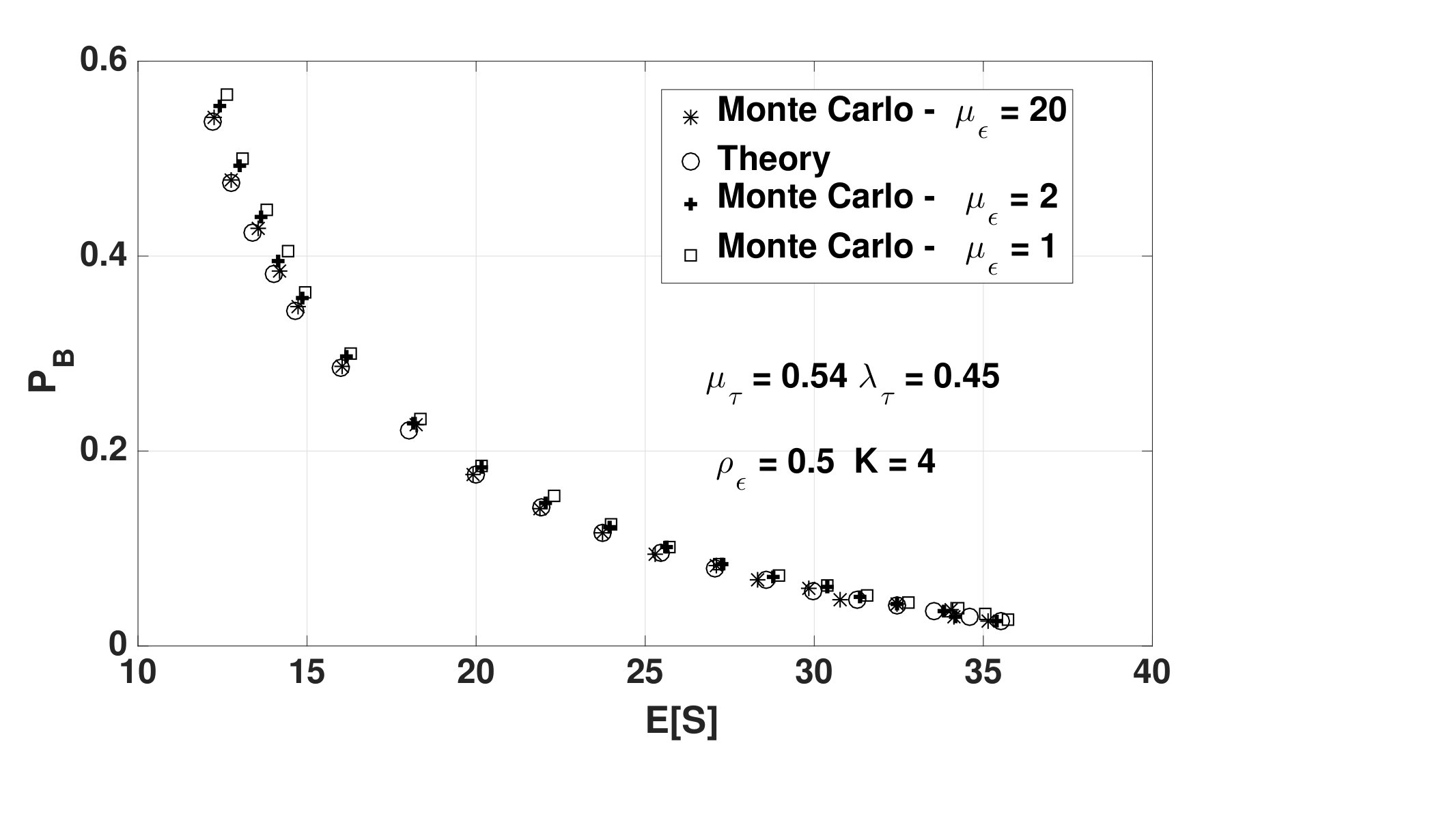 Figure 1
 Figure 2
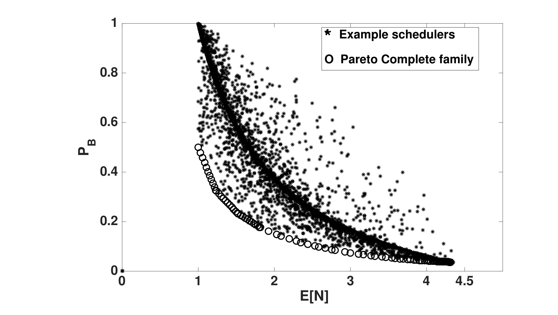 Figure 3
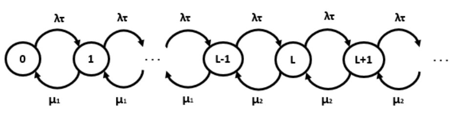 Figure 4
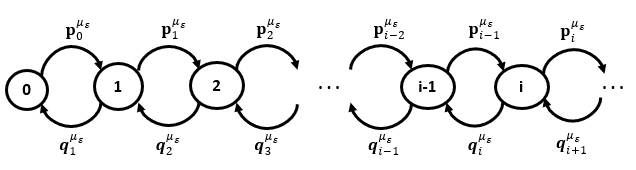 Figure 5
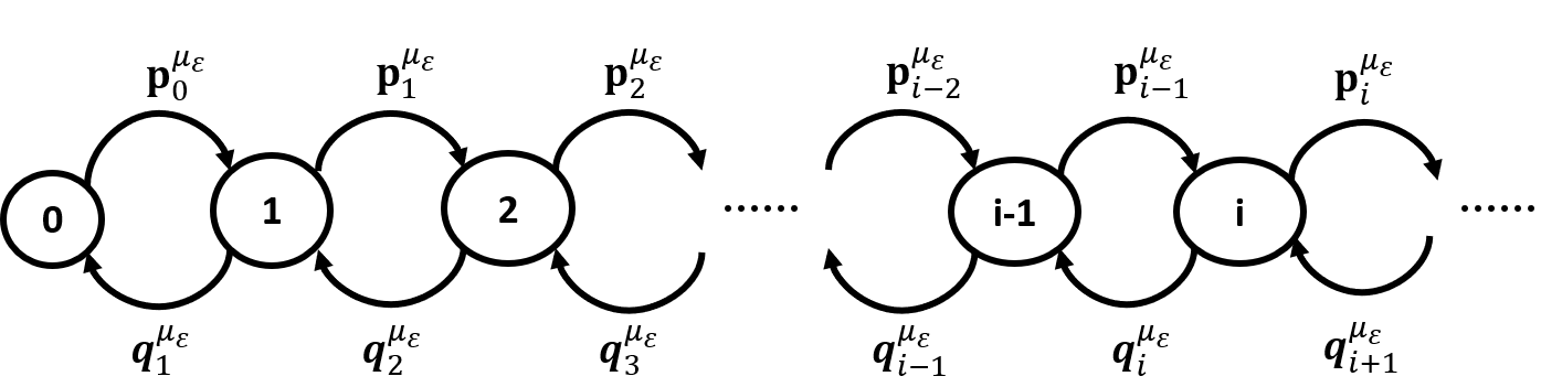 Figure 6
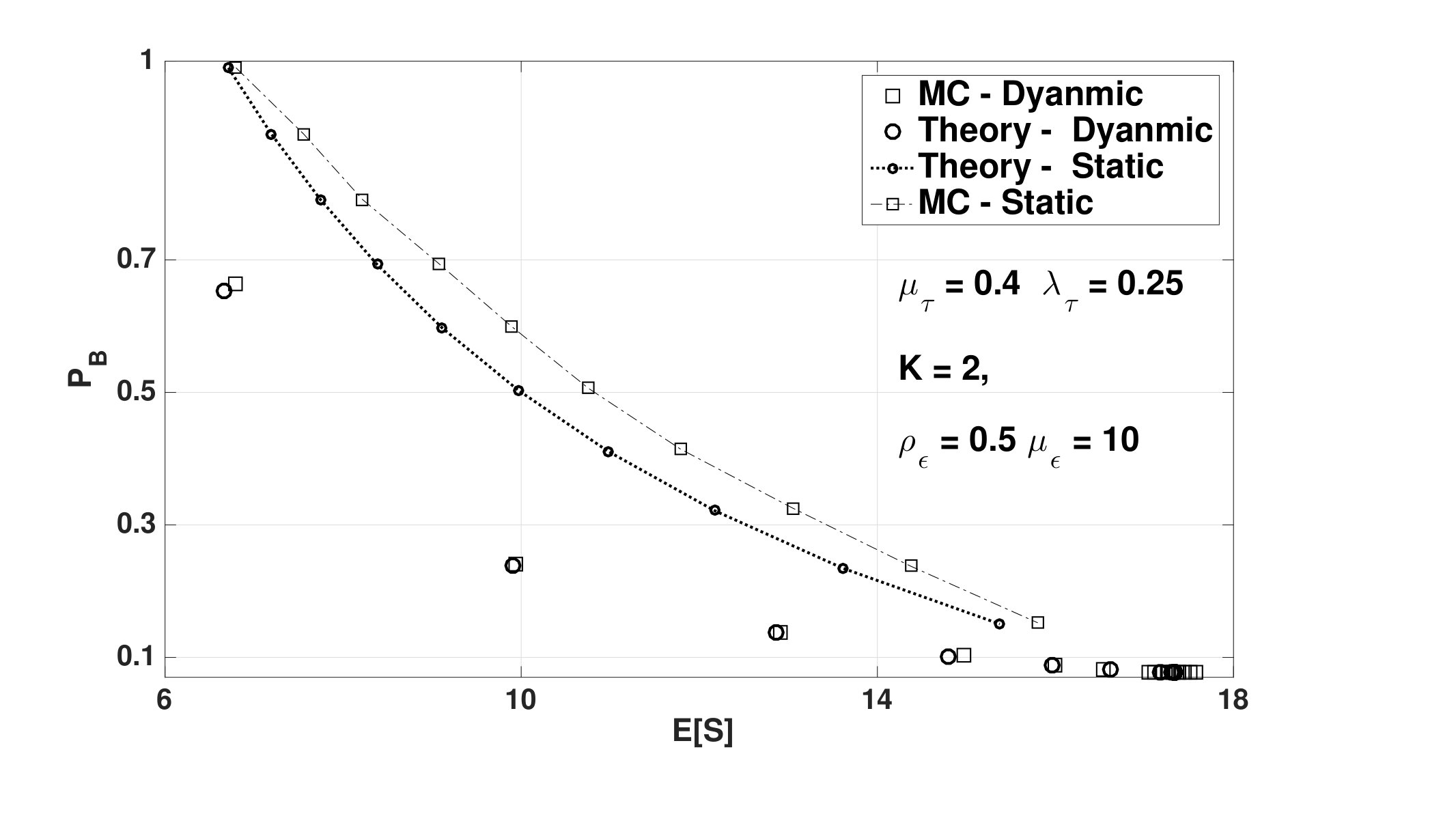 Figure 7
|
Basic Notations
|
|---|
| Poisson arrival rate of eager customer. |
| Poisson arrival rate of tolerant customer. |
| generic job size. |
| job-size at scale . |
| the load factor eager class. |
| inter-arrival time of tolerant customers. |
| Exponential job-size. |
| tolerant service rate when -sup-policy used for eager. |
|
Embedded chain
|
| : probability that tolerant arrival is before departure, in -system at occupancy . |
| : probability that -departure is before arrival. |
| : probability that -arrival is before departure, under limit system at occupancy . |
| : probability that -departure is before arrival. in limit system. |
| steady state probability that embedded -chain is in state , in -system. |
| steady state probability that embedded -chain is in state , in limit system. |
|
Continuous time process
|
| steady state probability that -process is in state , in system. |
| steady state probability that -process is in state , in limit system. |
| unused service process by class. |
| tolerant load when -sub -policy () used for eager. |
| time require to finish amount of work using . |
| standalone blocking probability when sub-policy used for eager class. |
| stationary expected number of -customer at system. |
| overall blocking probability at system. |
| overall blocking probability in limit system. |
| -busy cycle when sub-policy is used. |
| total service available for -class during . |
| -th -busy cycle when sup-policy is used. |
| total service available for -class during . |
Peer Reviews
No public reviews on file for this paper yet. If you reviewed it on a platform where reviews are public (OpenReview, ICLR, NeurIPS, ICML), you can paste yours below so the community can read it here.
Videos
No videos yet. Explain this paper in a talk, walkthrough, or lecture? Add one.
Taxonomy
TopicsAdvanced Queuing Theory Analysis · Advanced Wireless Network Optimization · Scheduling and Optimization Algorithms
Dynamic scheduling in a partially fluid, partially lossy
queueing system††thanks: A preliminary version of this work was presented at the WiOpt conference, 2019 [1].
Kiran Chaudhary Kiran Chaudhary and Veeraruna Kavitha are with the Industrial Engineering and Operations Research (IEOR) Department at IIT Bombay.
Veeraruna Kavitha22footnotemark: 2
Jayakrishnan Nair Jayakrishnan Nair is with the Electrical Engineering Department at IIT Bombay; he acknowledges support from DST and CEFIPRA.
Abstract
We consider a single server queueing system with two classes of jobs: eager jobs with small sizes that require service to begin almost immediately upon arrival, and tolerant jobs with larger sizes that can wait for service. While blocking probability is the relevant performance metric for the eager class, the tolerant class seeks to minimize its mean sojourn time. In this paper, we analyse the performance of each class under dynamic scheduling policies, where the scheduling of both classes depends on the instantaneous state of the system. This analysis is carried out under a certain fluid limit, where the arrival rate and service rate of the eager class are scaled to infinity, holding the offered load constant. Our performance characterizations reveal a (dynamic) pseudo-conservation law that ties the performance of both the classes to the standalone blocking probabilities associated with the scheduling policies for the eager class. Further, the performance is robust to other specifics of the scheduling policies. We also characterize the Pareto frontier of the achievable region of performance vectors under the same fluid limit, and identify a (two-parameter) class of Pareto-complete scheduling policies.
1 Introduction
In this paper, we analyse a single server queueing system with two heterogeneous customer classes. One class of customers is eager—they require service to commence (almost) immediately upon arrival. The performance of the eager class is captured by the blocking probability, i.e., the long run fraction of eager customers that are blocked. The second class of customers is tolerant—these customers can tolerate delays and may be queued. The performance of this class is captured via the mean response time of the tolerant customers.
Service systems of this kind are motivated by modern cellular networks, which handle voice calls (which must be either admitted or dropped upon arrival) as well as data traffic (which can be queued). Another motivation comes from super-markets, where it is common practice to provide prioritized service to customers with fewer items via dedicated express counters; these customers have limited patience, and may balk/renege if service is not provided almost immediately. However, such part-loss, part-queueing multi-class service systems are analytically intractable even under the simplest scheduling disciplines (see [2] and the references therein). In this paper, we derive tractable approximations of the performance experienced by each class using a certain fluid limit, referred to as the short-frequent-jobs (SFJ) limit.
The SFJ limit corresponds to scaling the arrival rate as well as the service rate of the eager class to infinity, such that the offered load is held constant. This gives rise to a time-scale separation between the two classes, the eager class operating at a faster time-scale. Under the SFJ limit, we obtain a closed form characterization of the performance of both classes under a broad class of dynamic policies that allow the admission control of the eager class and the scheduling of both classes to be dependent on the current state of the system.111From here on, we follow the convention that admission control (if used) is included in the eager scheduling policy. Interestingly, a dynamic pseudo-conservation law follows from this characterization (in the SJF limit)—the performance of both classes depends only on the standalone blocking probabilities (resulting when a single eager scheduling policy is used oblivious to the tolerant state) associated with the eager scheduling schemes employed for each occupancy level of the tolerant queue. In particular, the performance does not depend on the specific scheduling policies that generate those blocking probabilities, as well as on the details of the tolerant scheduler (subject to work conservation and serial, non-anticipative processing). Conservation laws typically allow one to compute the performance of a complex system in terms of the performance of simpler ones. In our case, once the relevant standalone blocking probabilities are known (these can usually be computed easily as they result from the analysis of a single-class loss system), one can compute the performance of both the classes.
We further analyse the Pareto frontier of performance vectors achievable under the class of dynamic schedulers, which defines the set of efficient operating points for the system. Remarkably, we are able to identify a Pareto-complete family of scheduling policies (we call a family of schedulers Pareto-complete if it spans the entire Pareto frontier over its parameter space). This family, parametrized by where and blocks eager customers with the minimum blocking probability when the tolerant occupancy is less than with probability when the occupancy equals and with the maximum blocking probability when it exceeds
Finally, via numerical experiments, we show that our performance characterizations under the SFJ limit are extremely accurate in the pre-limit (i.e., for moderate values of arrival and service rates of the eager class). This shows that our approximations, which are provably accurate under the SFJ fluid limit, are also applicable in practice.
The remainder of this paper is organised as follows. After a review of the related literature below, we describe our system model and state some preliminary results in Section 2. We also give some examples of dynamic schedulers in Section 2. Under the SFJ limit, we characterize the performance of the tolerant class and the eager class in Section 3. We formally define the dynamic achievable region in Section 4, and demonstrate the Pareto-complete family of dynamic schedulers in Section 5. We conclude the paper in Section 6. A summary of our notation can be found in Table 1 in Appendix A.
Related Literature
The present paper is a follow-up of our prior work [3, 4], which analyses the same heterogeneous queueing system under the SFJ limit for a class of (partially) static scheduling policies. Under this class of policies, the scheduling of the eager class is oblivious to the state of the tolerant queue, with the tolerant queue simply utilizing the service capacity left unused by the eager class. Clearly, this class of schedulers is restrictive. In the present paper, we consider general dynamic policies, where eager scheduling depends on the occupancy of the tolerant queue. This generalization, which requires a non-trivial analysis, results is a substantial expansion of the achievable region of feasible performance vectors (as is shown in Sections 4 & 5). Moreover, the generalization to dynamic policies necessitates the identification of a Pareto-complete family of schedulers (which is the goal of Section 5); within the restricted class of static schedulers analysed in [3, 4], it turns out that all policies are efficient.
Aside from [4, 3], the only prior work we are aware of that analyses a part-queueing, part-loss service system is [5]. In this paper, the authors obtain the performance metrics for all classes in closed form, assuming exponential inter-arrival and service times for all classes, under a certain static priority scheduling discipline. However, we note that [5] does not attempt to address the tradeoff between the performance of the two classes, which is central to the present work.
From an application standpoint, this paper is also related to the considerable literature on sharing the capacity of a cellular system between voice and data traffic; for example, see [6, 7, 8]. In this line of work, both voice and data classes are treated as lossy, the focus being on characterizing the blocking probability of each class under different (static and dynamic) admission rules. However, to the best of our knowledge, these papers do not analyse the achievable region of performance vectors, or characterize its Pareto frontier.
We also note that there is a well-developed literature on multiclass queueing systems with multiple tolerant classes on a single server (e.g., conservation laws, pioneered by [9]). The achievable region is well understood in such a ‘homogeneous’ multi-class setting [10, 11]. Interestingly, in this case, it is known that the static and dynamic achievable regions coincide (see [3]), in contrast with the ‘heterogeneous’ multi-class setting considered here, where we see that the static achievable region is a strict subset of the dynamic achievable region. Moreover, the achievable region in the homogeneous setting is its own Pareto frontier (i.e., all points of the achievable region are efficient) under work conserving policies, also in contrast with the heterogeneous setting considered here.
This paper is an extended version of [1], which analyses a restricted class of dynamic scheduling policies, wherein the number of distinct eager sub-policies is assumed to be finite. In this paper, we extend the analysis to general dynamic policies, and further provide complete proofs of all results.
2 System Description
We consider a single server queueing system with two job (a.k.a. customer) classes: eager customers (also denoted as -customers) demand service immediately upon arrival, whereas tolerant customers (also denoted as -customers) can wait in a queue (of infinite capacity) to be served.222We discuss the generalization where eager customers have limited patience and abandon/renege after a short wait time in Section 6; see also [4]. The -customers can be interrupted either partially (i.e., their service rate may be reduced) or completely by -customers, but not by other -customers. Without loss of generality, we assume a unit server speed. We assume that -customers (respectively, -customers) arrive according to a Poisson process with rate (respectively, ). The sequence of job sizes (a.k.a. service requirements) for both the classes is i.i.d., with denoting a generic job size, and denoting a generic job size. Throughout, we assume that is exponentially distributed with mean and that Let
2.1 Dynamic schedulers
We consider dynamic scheduling, wherein the scheduling policy for each class depends upon the state (occupancy) of both the classes. An eager scheduling (sub)policy (a set of rules that assign fractions of server capacity to various eager customers, which may also include the admission control rules) is chosen depending upon the tolerant state. The overall dynamic scheduler is characterized by a sequence of such eager sub-policies, one corresponding to each value of tolerant occupancy—the tolerant queue in turn utilizes the service capacity left unused by the eager class in a work-conserving manner. Our dynamic schedulers can thus be viewed to be of nested type: a top-level policy chooses the sub-policy used for scheduling the -class based on the occupancy (state) of the -class. The sub-policy in turn determines, based on the number of eager customers in the system, the admission rule for subsequent arrivals, and the service rate to allocate to each existing eager job. It is important to note that these nested schedulers are not restrictive; rather this is simply a convenient representation of dynamic schedulers; details and examples follow. As a result, the service processes of the two classes are interdependent (unlike in the case of static scheduling as considered in [4, 3]).
Specifically, let represent the number of tolerant and eager customers in the system at time . We consider stationary Markov scheduling policies that determine the service plan for both classes (including, possibly, admission control of eager customers), depending on the tuple Such Markov policies are known to be sufficient for a wide range of sequential decision problems (see [16]); in the context of our model, they are sufficient if one additionally assumes that eager customers have exponentially distributed service requirements. As an example, consider the following policy parameterized by : a) when with , and then each -customer is served with rate (speed) , while longest waiting -customer is served at rate ; and b) if , the longest waiting -customer is served with the full service capacity (i.e., at rate 1), and no further -customers are admitted. It is convenient to view such policies as being nested; for the above example, when the eager class is served according to one sub-policy, while it is served according to a second sub-policy when tolerant occupancy is more than . Under the former sub-policy, the eager class is served as an queue (with each ‘server’ taken to have speed ), while under the latter sub-policy, no eager customers are admitted. There is of course the issue of how to deal with the existing eager customers in the system when there is an arrival/departure in the queue, leading to change in the eager sub-policy. In the above example, this corresponds to the handling of any eager customers that remain when the occupancy increases from to This issue is addressed later in this section (see Assumption A.1 and the discussion in Section 2.3).
Note that the eager sub-policy switches whenever there is an arrival/departure in the tolerant queue, though the further details of each sub-policy depend only on the eager occupancy. We typically refer to the -sub-policy implemented when there are tolerant jobs in the system as sub-policy
-schedulers: Note that while the occupancy of the tolerant queue dictates the selection of the eager sub-policy, the sub-policies themselves are oblivious to the state of the tolerant queue. We make the following additional assumptions. Some examples of schedulers that satisfy these are presented in Section 2.3:
- A.1
To simplify the transition from one -sub-policy to the next, we assume that all -customers are dropped when there is an arrival/departure in the -queue. 2. A.2
The scheduling of each sub-policy depends only on the number of -jobs present in the system. 3. A.3
On arrival, an eager job is either admitted into service or gets dropped/blocked. If admitted, an eager job receives service at a minimum rate/speed of until its departure under any sub-policy.
Assumption A.1 is a technical condition required in our proofs. In Section 5, we show that this assumption has negligible influence on the performance of either class under our partial fluid limit.333 Under the SFJ limit, this ‘flushing’ of the -system is only performed at a bounded rate (since arrivals/departures in the -queue occur at a bounded rate), while the arrival rate of the system scales to infinity. Thus, we expect that this assumption will not impact the blocking probability of the eager class (this is also evident from the Monte Carlo simulation based study presented in Section 5). We are also able to relax Assumption A.1 for the special case of exponentially distributed eager jobs (see Theorem 4). As discussed before, Assumption A.2 is not restrictive; it allows all (non-size based) Markov policies. We provide examples of such schedulers in Section 2.3. Assumption A.3 implies that the eager class operates as a loss system. Indeed, the requirement of a minimum service rate/speed captures the ‘eagerness’ of eager customers. This assumption also implies that there exists a uniform upper bound on the number of -jobs in the system at any time across sub-policies (since the server is assumed to have a unit speed).
The above assumptions imply the following condition (proved as Lemma 3 in Appendix B.1); the same is stated as a (redundant) assumption to emphasize that the uniform convergence required in our analysis is predominantly due to the following uniform bound on the eager busy cycles:
- A.4
Across sub-policies, the second moment of the -busy cycle, defined as the interval between the start of two successive busy periods, is uniformly bounded.
-schedulers: Next, we state our assumptions on the scheduling policy of the tolerant class.
- B.1
The -scheduler is work conserving, i.e., it utilizes all the service capacity left unused by -jobs, so long as the -queue is non-empty. 2. B.2
The -jobs are served in a serial fashion, i.e., -jobs cannot pre-empt one another. 3. B.3
The -scheduler is blind to the size of -jobs.
Assumption B.1 implies that the tolerant class experiences a time varying service process, which depends on both the -state as well as the -state. Assumptions B.2-3 imply that we consider -schedulers which are non-pre-emptive and non-anticipative, for instance, first come first served (FCFS), last come first served (LCFS), and random order of service (see [12, Chapter 29]).
We require another assumption (B.4) regarding the stability of the -queue under the SFJ limit, when -customers employ a single sub-policy (irrespective of the -state). We provide the required background on these schedulers, define formally the SFJ scaling, and state the resulting pseudo-conservation law (see [4] for more details), after which we state Assumption B.4.
2.2 -static schedulers and background
We now consider the special case of -static scheduling, where a single -sub-policy is used at all times (irrespective of -state); this case was analysed in [4]. Let represent the blocking probability (long run fraction of losses) of the -class, if sub-policy- is used in a -static manner ( was referred to as the standalone blocking probability of sub-policy in Section 1); we also refer to these as -static blocking probabilities.
Short-Frequent Jobs (SFJ) Scaling: Under the SFJ scaling (as in [4]), we let and such that remains constant. This corresponds to scaling the arrival as well as the service rate of the eager class to infinity proportionately, so that the offered load (the long term rate at which work arrives into the system) is held constant. We use as the scale parameter for this partial scaling. Specifically, we scale the job size distribution of the eager class as, , where denotes a generic eager job size at scale and is equality in distribution. This scaling (plus Poisson arrivals) under A.2 ensures that at scale the occupancy process of the -class gets time-scaled (fast-forwarded) by the details can be found in Appendix A. Note that the tolerant workload remains unscaled. Thus, the SFJ scaling may be viewed as a time-scale separation, with the eager class operating at a faster time-scale.
Static Pseudo Conservation: Let represent the total amount of server capacity left unused by the -customers in time interval , under sub-policy operating in a -static manner. Note that is the (cumulative) service process seen by the -system. Then by [4, Lemma 1], for all the asymptotic (in time) growth rate of satisfies:
[TABLE]
In other words, the long run time average service rate seen by the -queue equals which depends only on the blocking probability of the eager class, and not on the specific -sub-policy that produced that blocking probability. Further under the SFJ limit, the service process seen by the -class becomes uniform. Specifically it follows from [4, Theorem 1] that, as in the SFJ limit,
[TABLE]
where denotes the time required to finish amount of work using the service process . This uniformity of the service process under SFJ limit enables a closed form characterization of the performance of the -class (see [4, Theorems 2,3]). A key feature of the above results is a pseudo-conservation law that expresses the performance of the tolerant class purely in terms of the blocking probability of the eager class, independent of the underlying -policy that produced the blocking probability. *We show an analogous pseudo-conservation for dynamic scheduling policies in this paper. *
Finally, we state the following assumption, which ensures that the -queue remains stable under each eager sub-policy, when they are applied in a -static manner.
- B.4
There exists such that
Assumption B.4 guarantees that the -system is stable in the dynamic setting as well, as is shown by Lemma 2.
2.3 Some example models
We begin with the description of one example system that satisfies our assumptions, in which the system capacity is not completely transferred to one class at any time, but rather a fraction of it is used by each -customer, whilst the left is utilized by one -customer.
Capacity Division (CD-) policy: Each -customer uses part of the service capacity. If there are number of -customers receiving service, then -customers are served at a net service rate of , while the -customer in service (if any) is served at rate . This continues up to -customers, and any further -arrival departs without service. Note that whenever an existing -customer departs, the service rate of the -customer gets increased by . Of course, to satisfy Assumption A.3. Further there is a prior admission control on -arrivals, they are admitted with probability independent of all other events. This is the description of the -sub-policy (as in [3, 4]). Now the top-level policy varies the probability of admission (and possibly the maximum occupancy ) based on the occupancy of the -queue.
We refer to the above -sub-policy as Capacity Division or briefly as the CD- policy. Note that the CD- policy captures a multi-server setting for the eager class. While the -scheduler need not be work conserving, the -class uses all the left over capacity. Another example of an -sub-policy is the following.
Limited Processor Sharing (LPS-) policy: This sub-policy, denoted by LPS- (as in [3, 4]), admits an incoming eager job into the system with probability so long as the number of eager jobs already in service is less than or equal to The entire service capacity of the server is shared equally between the eager jobs in service (i.e., each eager job gets served at rate when there are jobs in service). As before, Note that under the LPS- policy, the tolerant class receives service only when there are no eager jobs in the system.
Top-level policies: The top-level policy can chose any one of these sub-policies for any -state. For example, when the -occupancy is greater than a certain threshold one may allocate fewer individual servers to -customers (using, for example, the CD policy), while one may allocate the entire capacity to the -class and may serve them in LPS mode when the -occupancy is smaller.
Switching between sub-policies: Note that under Assumption A.1, the transition between sub-policies, triggered by an arrival/departure in the queue, is simplified—any left over eager jobs at the time of the transition are simply ‘flushed’. This simplifies our analysis, and as argued before, would have a negligible impact on the performance of both classes in the SFJ scaling regime. In practice, a more natural implementation strategy would be to simply let the new sub-policy dictate the scheduling of the existing eager jobs in the system after the change of the occupancy. This implies a possible re-assignment of the service rates of eager customers at the time of the -transition. We prove formally that doing this does not affect our main results under the SFJ limit, for the special case of exponentially distributed eager job sizes (see Theorem 4).
3 Performance Characterization under the SFJ limit
In this section, we characterize the performance of the -class and the -class under the SFJ limit.
Recall that in our system, both classes are scheduled in a dynamic manner, with the -sub-policy being selected based on current -occupancy, and the -queue in turn being served (in a work conserving fashion) using the unused service process of the -sub-policy. Thus, the two classes experience random, time varying, state-dependent, and also inter-dependent service processes. This makes a precise performance evaluation intractable; indeed, no closed form characterization of the performance of the tolerant class is possible even in the simplified setting where the eager class is scheduled by a policy that is oblivious to the tolerant state; see [2, 4]. In this section, we show that under the (partially fluid) SFJ scaling, tractable performance characterizations are possible.
To provide intuition for the form of our results, recall that the timescale separation resulting from the SFJ scaling results in the tolerant queue obtaining, in the limit, service at a ‘steady’ rate of when there are tolerant jobs in the system. Here, is the standalone, or -static blocking probability associated with sub-policy One might then anticipate that the limiting performance of the tolerant class is described in terms of a system with a state-dependent service rate, i.e., where the service rate is a (deterministic) function of the queue occupancy. We prove that this is indeed the case. Before we state our main results, we first describe this limit system, which we refer to as a state-dependent service rate M/M/1 (SDSR-M/M/1) queue.
3.1 State-dependent service rate M/M/1 queue
An SDSR-M/M/1 queue sees the same arrival process as an M/M/1 queue: job arrivals are according to a Poisson process (of rate ). Further the job sizes are independent and exponentially distributed with mean . However, unlike the standard M/M/1 queue, the SDSR-M/M/1 queue has a state dependent service rate (a.k.a. server speed). Specifically, the server operates with service rate if the number of jobs in the queue (including the job in service) equals Thus, the SDSR-M/M/1 queue is parametrized by , where is the vector of service rates.
The number of jobs in the SDSR-M/M/1 queue evolves as a continuous time Markov process with birth-death structure (see Figure 1).
Moreover, Assumption **B.**4 ensures that this Markov process is positive recurrent. Thus, its steady state distribution can be obtained by elementary techniques. In particular, the stationary distribution , is given by (see [13]):
[TABLE]
3.2 Main results
Recall that the scheduler is specified by a sequence of eager sub-policies one for each tolerant occupancy; being the -static probability of the eager sub-policy used under tolerant occupancy . The performance of the tolerant class under the SJF limit, and under any scheduler, is characterized as follows. The steady state occupancy of the tolerant queue converges, in distribution, and also in expectation, to the corresponding quantities of an SDSR-M/M/1 system parameterized by
Theorem 1**.**
[Stationary distribution of -occupancy]*
Assume .1-4 and .1-4. Under the SFJ limit, the steady state number -occupancy converges in distribution to the steady state occupancy in an SDSR-M/M/1 queue, with*
[TABLE]
That is,
[TABLE]
where is given by (3).
Theorem 2**.**
[Stationary expected -occupancy]*
Assume .1-4 and .1-4. Under the SFJ limit, the stationary expected number of -customers converges to that of the limit system described in Theorem 1. That is,*
[TABLE]
where is given by (3).
Given that is the stationary distribution of a simple birth-death CTMC, Theorems 1 and 2 provide closed form characterizations of the limiting performance of the tolerant class under the SFJ scaling. It is important to note that while the statements of Theorems 1 and 2 might seem intuitive, their proofs are rather involved. In particular, they rely crucially on a uniformity in the convergence of the service process seen by the tolerant queue under the SFJ limit, across -sub-policies; see Subsection 3.3.
Next, we describe the performance of the eager class under the SFJ limit, which is captured by its blocking probability, i.e., the long fraction of eager customers blocked. Formally, the blocking probability is defined as follows. Let denote the total number of eager customers that are blocked (i.e., returned without service), before time and be the total number of eager customers arrived in the same time interval, for the system at scale Then the blocking probability of the eager class is defined as the long run fraction of customers blocked, i.e.,
[TABLE]
Note that eager jobs are blocked by different sub-policies, which operate dynamically based on the occupancy of the tolerant queue. Thus, it is not a priori even clear that the limit in (4) exists almost surely. That it does, and that the eager blocking probability converges under the SFJ limit to a convex combination of the -static blocking probabilities weighted by the (limiting) long run fractions of time the -system spends in each state, is established by the following theorem.
Theorem 3**.**
**[Blocking probability of eager class]
Assume A.1-4, B.1-4. Then the steady state blocking probability of -jobs in SFJ limit is given by:**
[TABLE]
where is given by (3).
A key takeaway from Theorems 1–3 is that the performance of both classes under the SFJ limit can be characterized in terms of the -static blocking probabilities . The probabilities themselves are typically easy to compute, since they involve the analysis of a single-class (stationary) loss system. Thus, by virtue of Theorems 1–3, we have the following conservation law.
Dynamic Pseudo Conservation: Under the SFJ limit, the performance of both classes depends only on the -static blocking probabilities and not the specifics of the -sub-policies that produced these blocking probabilities.
Finally, since Assumption A.1 may seem unreasonable, we show below that the conclusions of Theorems 1-3 hold even without this assumption, if eager job sizes are taken to be exponentially distributed.
Theorem 4**.**
Assume A.2-4 and B.1-4. Also assume that the -service times are exponentially distributed. The conclusions of Theorems 1-3 hold, once the transitions between eager sub-policies are handled as described in Section 2.3 (i.e., following an arrival/departure in the tolerant queue, the new eager sub-policy dictates the scheduling of the eager queue from then on).
Theorem 4 shows that Assumption A.1 is benign, i.e., it does not affect the performance of either class under the SFJ limit. As expected, the proof of Theorem 4 is considerably more involved as compared to the proofs of Theorems 1-3. Specifically, Assumption A.1 allows the evolution of the queue (across arrival/departure epochs) to be described by a one-dimensional birth-death Markov chain (see Section 3.3). This is no longer possible in the absence of Assumption A.1; the system evolution has to be captured via a certain two-dimensional Markov chain, whose long-run time averages must be shown to match those corresponding to the former birth-death chain as (see Appendix D).
We note that while our performance characterization is derived under the SFJ limit, we show in Section 5 that they provide accurate approximations of the performance experienced in the pre-limit. The remainder of this section is devoted to highlighting the main steps in the proofs of Theorems 1 and 2. Most details are relegated to Appendix B. The proof of Theorem 3 is presented in Appendix C. The proof of Theorem 4 can be found in Appendix D.
3.3 Analysing tolerant performance under the SFJ limit
We now sketch the main steps in the proofs of Theorems 1 and 2 (i.e., under Assumption A.1). We characterize the -performance by first analysing the -queue at its arrival/departure epochs. Let denote the occupancy of the -queue immediately following the th arrival/departure. Under Assumption A.1 (dropping of existing -customers at -transitions) and because of exponentially distributed tolerant job sizes, is a discrete-time Markov chain with birth-death (BD) structure; see Figure 2. Let and , respectively, denote the forward and backward transition probabilities of this (pre-limit) tolerant BD chain, when there are tolerant customers in the system. Let and represent, a generic inter-arrival time associated with the tolerant queue, and a generic tolerant job size, respectively. Also, recall denotes the time required to finish amount of work using the service process (see Section 2.2), then we have:
[TABLE]
Observe by A.1 that the job completion times, distributed as , are i.i.d. across all those customers that were served when the tolerant occupancy equals . Moreover, if such a tolerant service is interrupted by a -arrival, the remaining completion time is distributed as thanks to the memoryless property of tolerant job sizes and A.1.
Our first step is to prove that the above transition probabilities converge to the transition probabilities associated with the embedded BD chain corresponding to the SDSR-M/M/1 system. Moreover, we show that the above convergence takes place uniformly over sub-policies Before stating this result, we recall the definition of uniform convergence (which we denote by ):
Definition: \left[\textbf{Uniform (u.f.) convergence }\right] A parameterized family of sequences is said to be uniformly convergent to the limit as if, for every there exists , such that
[TABLE]
Lemma 1**.**
* i) If denotes the probability of a -arrival before a -departure in the (pre-limit) system when the number of tolerant customers in the system equals , then*
[TABLE]
ii) The convergence in (5) occurs u.f. over the sub-policies . Precisely, for every there exists , such that for all and for all we have:
[TABLE]
The proof of Lemma 1 is provided in Appendix B.2.
The next step is to show that the embedded BD chain characterizing the evolution of the occupancy of tolerant queue is positive recurrent for large enough
Lemma 2**.**
There exists such that for the (embedded) Markov chain is positive recurrent.
The proof of Lemma 2 is provided in Appendix B.3. Lemma 2 also implies that for large enough the -queue is stable and has a well defined stationary behaviour.444The occupancy of the tolerant queue evolves as a semi-Markov process in continuous time. The regularity of this process (i.e., each state is visited only finitely often in any finite interval of time with probability 1) follows by noting that the number of state transitions is lower bounded by those in a standard M/M/1 queue with arrival rate and service rate . The positive recurrence of this process follows from Theorem 5.9 in [13], noting that mean residence time in any state is uniformly upper bounded by The stationary distribution for can be calculated using standard techniques and is given by (see, for example, [14]),
[TABLE]
with defined as:
[TABLE]
Now, given that the embedded BD chain capturing the evolution of the tolerant queue is positive recurrent for large enough (Lemma 2), and has transition probabilities that converge (under the SFJ limit) uniformly to those of the embedded chain of the SDSR-M/M/1 queue (Lemma 1), we can now establish convergence of the stationary distribution of this embedded process to that of the SDSR-M/M/1 system as well.
Theorem 5**.**
*
Under SFJ limit, the stationary distribution of the embedded (BD) chain corresponding to the tolerant Markov process given by equation (7) and (8) converges to that of the SDSR-M/M/1 queue with variable service rates. That is,*
[TABLE]
where, is given by (3).
Note that Theorem 5 deals with the limiting behavior of the embedded chain corresponding to the (continuous time) occupancy process of the tolerant queue. Our main results Theorems 1 and 2 can be proved from Theorem 5 by invoking a relationship between the stationary distribution of an embedded Markov chain and that of the corresponding continuous time process (see Lemma 8 in Appendix B.5); the details can be found in Appendices B.5 and B.6.
4 Dynamic Achievable Region
A queuing system can be analysed using several performance metrics; for example, number of customers in the system, sojourn time (the total time spent by the customer), waiting time (of the customer before the service starts), fraction of the customers blocked (in a loss system), etc. The achievable region of a multi-class system is defined as the region of all possible vectors (one component for one class) of the relevant performance metrics.555In this paper we consider the achievable region corresponding to schedulers which satisfy Assumptions **A.**1-4 and **B.**1-4. In our model, corresponding to the eager class we have a lossy system, thus we consider blocking probability as the performance metric. For the tolerant class, one can consider the steady state expected number of customers in the system as the performance metric.
By Lemma 2, the system is stable for all , for some . Thus for all such , by Little’s Law, the stationary expected sojourn time of a typical -customer, and the stationary expected number of -customers in the system are related as Thus it is sufficient to consider any one of these metrics.
Stationary Markov top-level policies: In any general sequential decision problem, a Stationary Markov (SM) policy is a sequence of decisions, in which one decision is chosen for each value of the state and the same decision is applicable in any time slot. In our case we consider the top-level policies among the Stationary Markov (SM) family. This means, a top level policy is a sequence of -sub-policies, and that if the -state equals at any time slot, then the -th sub-policy of is used for scheduling the -class.
As understood from Theorems 2-3, the only characteristic of the -sub-policies that influences the system (dynamic) performance are the -static blocking probabilities , obtained when respective sub-policies are used in -static manner. Thus to define an efficient dynamic system, one effectively needs to choose (based on the -state), one among these blocking probabilities (and no further details of the sub-policy are important). This is a consequence of the ‘dynamic pseudo-conservation’ mentioned in the previous section.
Any Stationary Markov (SM) top-level policy is generally given by a sequence of -sub-policies, one for each -state. However, in view of the above observation, a stationary Markov policy can be thought of as a sequence of -blocking probabilities (derived when the corresponding sub-policies are applied in -static manner. In other words, a SM top-level policy is defined by , where decision specifies a ‘-static blocking probability’ to be chosen when number of -customers equals . Towards this we implicitly require the existence of at least one sub-policy, that achieves the given value of ‘-static blocking probability’, which is any value between the system specified limits (minimum possible blocking probability) and (the maximum possible blocking probability). This for example, is achieved by CD-/LPS- policies mentioned in Section 2, when one considers all possible values of (see [3, 4] for more details). In the rest of the paper, we refer to the top-level policies simply as policies for brevity.
Limit Achievable region Our focus from here on will be the dynamic achievable region of performance vectors under the SFJ limit. Recall that for tolerant class, the limit is an SDSR-M/M/1 queue. The -limit can be seen as a mixture model made up of many lossy systems, each described by their -static blocking probabilities, and mixed independently according the stationary distribution of the limit SDSR-M/M/1 queue. Thus, we define the limit achievable region as follows:
[TABLE]
Note that is the set of limiting performance vectors under SM policies. In this sense, one may view as the limit of achievable region of our multi-class system as
For simplicity of notations we avoid the super-script when the discussion is clearly about the limit system. At times we also drop , the SM policy, when there is no ambiguity.
A Numerical Example: To visualize the limit achievable region, we consider a system with a top-level policy parametrized by (). In this system, the CD- policy is employed when the -occupancy is less than and the CD- policy is employed when the -occupancy is greater than or equal to The tolerant customers are served serially with total capacity of all the leftover servers. Using the Erlang-B formula, the two -static blocking probabilities of -customers equal
[TABLE]
where is the -static blocking probability when -occupancy is less than , while is the -static blocking probability for the rest of the tolerant states. The performance of such a system at limit can be obtained using the results of Theorems 2-3. We set , , and , generate the three parameters randomly. The scatter plot of the corresponding values of and is shown in Figure 3. The resulting figure is a part of the limit achievable region. As seen from the figure, the achievable region is a non-zero measure set; thus we need the ‘efficient’ Pareto frontier. Further, the plot indicates that the achievable region is bounded. We will now address the Pareto frontier associated with this system.
5 Limit Pareto frontier
The Pareto frontier is the efficient sub-region of an achievable region which consists of dominating performance vectors. A pair (produced by a policy ) is on Pareto frontier of the limit system, if there exists no other SM policy that achieves a better performance pair (in the limit system), i.e., one of the inequalities being strict.
The Pareto frontier of the limit system is obtained by solving an appropriate set of parametrized optimization problems. Prior to that, we discuss the limit performance, under any given SM policy. Invoking Theorems 2 and 3, under any ,
[TABLE]
5.1 Pareto-complete family
We now derive a family of Pareto-complete policies, i.e., a parametrized family of policies that span the entire Pareto-frontier of our system. One can obtain all the points on the Pareto frontier by considering the following parametrized (by ) constrained optimization problems (with defined in (11)). l
[TABLE]
Recall , respectively represent the best and worst sub-policy (with respect to -customers), in that these represent the minimum and maximum possible blocking probabilities. Define:
[TABLE]
The terms represent the (worst and best) load factor of the -customers in the limit system, when -customers are scheduled respectively with the best (blocking probability ) and worst (blocking probability ) sub-policies, in -static manner.
Suppose that the constraint on the expected -number satisfies (observe is the expected number in M/M/1 queue with maximum load factor ); then the problem (12) becomes an unconstrained problem and the optimal policy clearly equals . We show that the optimal policy for any given , is monotone (but not strictly monotone) in -state and further derive its closed form expression (proof in Appendix E):
Theorem 6**.**
The policy that optimizes the problem defined in (12) is monotone and is given by:
[TABLE]
which is parametrized by two parameters . The expressions for are given by (see (13)):
[TABLE]
In the above , is set to when the inequality defining the is satisfied for all (i.e., when ).
An immediate consequence of the above theorem is the following:
Corollary 1** **(Pareto-Complete family).
The family of schedulers given by (14), parametrized by with and , is Pareto-complete.
The policies in this family choose the ‘worst’ -sub-policy (i.e., with ) when the -number is greater than or equal to , choose a sub-policy with intermediate blocking when -number equals and choose the ‘best’ sub-policy (i.e., with ) for the rest (see (14)). One can easily compute the performance under these policies, as below (see 13):
[TABLE]
Thus *we derived Pareto complete family as well as the performance under this family, which can readily be used for any relevant optimization problem. *
Numerical example: We continue with the numerical example of Figure 3. For this example, one can easily compute that (no admission control on eager class, i.e., with for all ) and (eager class is completely blocked with and hence ), when the system can at maximum serve 5 eager customers in parallel. By substituting these values into (5.1), one can obtain the Pareto frontier. The circles in the figure represent this Pareto frontier, and are obtained by varying appropriately. It is clear from the figure that the derived set of points are indeed dominating and are on the Pareto frontier.
5.2 Monte Carlo based case study in pre-limit
We consider an example case-study with CD- sub-policies of Subsection 2.3. Specifically, for fixed we consider top-level policies that perform CD- when the -occupancy is less than certain (with ) and perform CD- (thus blocking all -jobs) when the -occupancy is greater than or equal to In view of Theorem 6, by stepping over as above666 Here again, (respectively ) equals the blocking probability without eager admission control (respectively if eager class is admitted only when -queue is empty)., we sample performance vectors from the limit Pareto-frontier of the system.
It is very complicated to obtain an exact analysis of this heterogeneous system. However by Theorems 2-3, one can obtain an approximate analysis for this system. In this section, we validate these approximations against Monte Carlo (MC) simulations of the actual system. Importantly, the Monte Carlo simulations do not even drop -customers at -transitions as required by A.1.
In all the case studies presented in this section, we consider exponentially distributed job sizes and Poisson arrivals for both the classes. The parameters used for a particular case study are described in the corresponding figure itself.
Our first case studies are presented in Figures 5 and 5. We plot two performance measures, mean number of tolerant jobs, and blocking probability of eager jobs, versus for two different tolerant load factors; Figure 5 corresponds to a light tolerant load, while Figure 5 corresponds to a moderate tolerant load. (The system parameters used are mentioned in the figures directly.) Note that as expected, the simulated system performance metrics approach their SFJ approximations as increases. Interestingly, our approximations tend to under-estimate both metrics (perhaps because the partial fluid limit we consider ‘washes away’ the stochasticity of the eager workload). Moreover, note that in the case of moderate tolerant load, the approximation is quite accurate for all values of ; the normalized difference between the theoretical approximation and the corresponding MC estimate is within for with and for with and the error is negligible for higher values of (see Figure 5). On the other hand, with light tolerant traffic () as in Figure 5, the normalized difference is within only for for and only for for . In general, we observe that the approximation error is smaller when the system operates closer to its stability limit. But even for the case with light traffic, the normalized difference is within in most cases once
Next, we consider the Pareto frontier of performance vectors, and compare our SFJ approximation with the frontier obtained via MC simulations; see Figure 7 . We observe that our analytical results corresponding to the SFJ limit provide a very accurate approximation of the Pareto frontier, even for as small as 1, when . We reiterate that the theory approximates the system performance well even when the system does not ‘flush’ -customers at -transitions.
Another example is plotted in Figure 7, where -static policies of [4] are considered along with dynamic policies. We again observe a good approximation between the theory and MC estimates for dynamic policies. Interestingly, the approximation error is bigger in the static case. One possible explanation for this is the following. It is clear that the approximation error gets smaller as the -load factor reduces, under -static policies. Under Pareto optimal family of schedulers, the -load equals 0 for all -states greater than . Thus we see the approximation is almost zero towards the right of the two figures (as gets smaller, gets smaller). We also observe that the dynamic policies perform far superior than -static policies.
6 Concluding remarks
In this paper, we analyse a multi-class, single server queueing system with an eager (lossy) class and a tolerant (queueing) class, under dynamic scheduling. While the inter-dependence between the service processes of the two classes makes an exact analysis of this system difficult, we obtain tractable performance approximations under a certain (partial) fluid scaling regime. A key feature of our approximations, proved to be accurate under the fluid limit, is a pseudo-conservation law: the approximate performance of both classes is expressed in terms of the standalone blocking probabilities of the eager schedulers, which are themselves easy to compute in several cases. Further, the accuracy of our approximations in the pre-limit is validated via Monte Carlo simulations.
Finally, we focus on the achievable region of the limiting performance vectors for our system. Remarkably, we are able to obtain an explicit family of Pareto-optimal policies (these resemble threshold policies).
There are natural extensions of our results to models where the eager class exhibits limited patience; for example, models with balking and/or reneging. For example, the system might include (limited) waiting room for eager customers. Alternatively, eager customers might respond to the resources allocated based on their patience levels: a) an -customer may not enter the system depending upon the -number already in system according to some probabilistic rule, as in balking models; or b) may leave the system after waiting for a random ‘patience time’, as in reneging models. At their core, our proofs require the property that the occupancy process of the eager class gets time-scaled (fast-forwarded) with increasing under the SFJ scaling. The analyses apply to the above mentioned generalizations so long as this scaling property holds. For example, in the case of reneging, we would require that the patience time distribution is scaled suitably with (as is discussed in the context of static scheduling in [4]).
This work also motivates extensions in other directions. One interesting extension would be to the multi-server setting, where the tolerant class is no longer work conserving. Another promising direction is to consider static/dynamic pricing for such heterogeneous service systems. Finally, specializing our models to particular application scenarios, including supermarkets, cognitive radio, and cloud computing environments, would be of independent interest.
Appendix A Sample path coupling and SFJ limit
In this appendix, we detail the sample path coupling that results from the SFJ limit, which is central to our arguments.
We consider a family of queuing systems, parametrized by (the service rate of the -class). Under SFJ limit, the eager service rate , and the eager arrival rate while maintaining the eager load to a constant value. Specifically, we scale the job size distribution of the eager class as, , where denotes a generic eager job size at scale and is equality in distribution.
Consider now this family of queueing systems, immediately following an arrival/departure from the tolerant queue. Specifically, suppose that the arrival/departure resulted in jobs remaining in the tolerant queue. We couple the sample paths across different values of the scale parameter as follows. Let and are respectively the th inter-arrival time and th job size of the eager class under sub-policy (for notational convenience, the dependence on is suppressed here). We relate these quantities sample path wise to the system as below:
[TABLE]
Note that this coupling is consistent with the SFJ scaling: is indeed exponentially distributed with mean given that is exponentially distributed with mean Similarly, note that we have as required.
An immediate consequence of (16) is that the occupancy process of the eager class at scale can be viewed as a -time-scaled (or fast-forwarded) version of occupancy process at scale 1; see [4] for more details. In particular, let and denote the length of the th -busy cycle (the interval between the start of two successive -busy periods), and total service available for the -class during the th -busy cycle, respectively, when tolerant queue occupancy equals It now follows that
[TABLE]
We conclude by describing another consequence of the sample path coupling (16) described above. Let represent the number of -arrivals in time interval and let represent the number of drops (or the -customers that exit the system without service) in the interval when sub-policy is used in a -static manner, at scale . More compactly, let , represent and respectively. Then, by the way of construction:
[TABLE]
and a similar equality holds for subsequent -busy cycles as well. These kind of consequences play a central role in deriving the results of the next two appendices.
Appendix B Tolerant Performance
In this appendix, we provide proofs of the results stated in Section 3, corresponding to the performance evaluation of the tolerant class.
This appendix is organized as follows. In Section B.1, we prove a technical result that is used to prove Lemma 1. The proofs of Lemmas 1 and 2 are provided in Sections B.2 and B.3, respectively. The proofs of Theorems 5, 1 and 2 are provided in Sections B.4, B.5, and B.6, respectively.
B.1 Bounding the second moment of -busy cycles
To prove Lemma 1, we need the following technical lemma, which states that second moment of the the eager busy cycles corresponding to -occupancy and scale are uniformly bounded from above over sub-policies
Lemma 3**.**
*Under Assumptions ***A.**1-3, Assumption A.4 is true, i.e., there exists a constant such that for any sub-policy
Proof.
Note that busy cycle where denotes the busy period, and the idle period between two successive busy periods. Moreover, is exponentially distributed with mean Thus, to prove the statement of the lemma, it suffices to prove that is bounded from above uniformly over sub-policies This is proved as follows. The busy period under any sub-policy can be upper bounded by the busy period of an system with arrival rate and job size Indeed, note that since any admitted eager job of size must be served at a minimum rate of is an upper bound on the residence time of the job in the system. The statement of the lemma now follows from Lemma 4 below, which provides an upper bound on the second moment of an busy period. ∎
Lemma 4**.**
Consider an queue with arrival rate with a generic job size denoted by . Let denote a generic busy period of this system. Then
[TABLE]
where
Proof.
Given a non-negative random variable having finite expectation, let denote its forward excess, i.e., is a non-negative random variable satisfying
[TABLE]
Note that
Now, returning to the queue, let Define a non-negative random variable , which is distributed as below:
[TABLE]
Finally, let denote a geometric random variable such that
[TABLE]
The following representation for the forward excess of the busy period was established by Makowski [15]:
[TABLE]
where is an i.i.d. sequence of random variables distributed as independent of
From (20), we have
[TABLE]
which yields
[TABLE]
Here, we have used which is also proved in [15].
We upper bound as follows. Using the Markov inequality, It then follows that for Now,
[TABLE]
The bounding in uses the inequality for with (by convexity of ). Finally, combining (21) and (22) gives us the statement of the lemma. ∎
B.2 Proof of Lemma 1
Recall that, when -occupancy equals (for any given ), the backward transition probability of the tolerant birth-death chain (at scale ) is given by . We aim to show the convergence of these transition probabilities, uniformly over , under the SFJ limit. The idea is to develop (for each ) a lower and an upper bound on which uniformly converge to the same constant given by Equation (5).
Consider the evolution of the tolerant queue, starting from an instant when the occupancy changed, via an arrival or a departure, to Let denote the time until the next arrival, let denote the th -busy cycle and let denote the total amount of service available for the tolerant class during the th -busy cycle, at scale
Lower bound: Consider any eager sub-policy . Define Note that is the index of the -busy cycle in which the next arrival occurs. Since is exponentially distributed, is a geometric random variable with parameter Further, define Note that which is the service received by the queue in the first -busy cycles, is a lower bound on the total service received by the queue until the next -arrival. Thus, the event implies that a - departure would precede the next -arrival; this yields the bound Moreover, the lower bound , on can be represented as follows:777Let , with indicator of the event . Condition on the events of first -busy cycle:
•
if and then ; otherwise
•
if then ; or
•
if and , then the conditional probability of equals its unconditional probability by the memorylessness of and .
And thus,
which implies (23) given that
[TABLE]
By Lemma 5 below, we have uniform convergence (here, as u.f. in ):
[TABLE]
where is a typical -busy cycle and is the (typical) unused service left behind by the eager class in one -busy cycle, both with and under sub-policy . Using the above and because888When renewal reward theorem is applied with renewal cycles as -busy cycles and with rewards being the amount of service available to the -class in each busy cycle. , we get from equation (23) that the lower bound on ,
[TABLE]
Upper bound: Next, we will prove the u.f. convergence of an upper bound on the transition probabilities , to the same limit. Since , one can upper bound as follows:
[TABLE]
In view of Lemma 6 below, we have as ,
[TABLE]
Therefore the upper bound on ,
[TABLE]
This proves that the lower and upper bound converge to the same limit (for any given ), uniformly across all . This proves the statement of the lemma. ∎
Lemma 5**.**
*We have:
i) and
ii)
That is, there exists a function (which is independent of and is finite by Lemma 3), such that as and for each ,*
[TABLE]
Proof.
Proof of : Note that, for any random variable the moment generating function (MGF) is given by: We use the following bounds in our proof repeatedly. Suppose that the random variable is exponentially distributed with mean and the random is non-negative and independent of Then
[TABLE]
The equality above follows by conditioning on and the inequalities are a consequence of the following bounds on the MGF: for
[TABLE]
Now, since is exponentially distributed and because (see (17)), we have, using (24),
[TABLE]
Using this inequality, and invoking (24) again,
[TABLE]
This completes the proof of Part .
Proof of (ii): Again, since is exponentially distributed, using (24), we have
[TABLE]
Since, , we will have
[TABLE]
Because and are exponentially distributed, the second term of the above inequality becomes (using the lower and upper bounds on as before):
[TABLE]
The result follows from (25), (26), and (27):
[TABLE]
This completes the proof of lemma. ∎
Lemma 6**.**
The probability converges to 0 u.f. over , under the SFJ limit.
Proof.
Using arguments similar to those in the proof of Lemma 5 (see equation (24)), we can prove that
[TABLE]
From this and (27) we will have,
[TABLE]
The statement of the lemma now follows by the uniform bound on (Lemma 3). ∎
B.3 Proof of Lemma 2
By Lemma 7 below, for any , there exists a such that for
[TABLE]
where the last inequality is shown in the proof of Lemma 7 . Thus by standard text book arguments (e.g., [14]) we have the result. ∎
Lemma 7**.**
*Assume the hypothesis of Lemma 1. Then we have following under SFJ limit:
(i) , u.f. over ,
(ii) , u.f. over ,
(iii) .
(iv) .*
Proof.
By Lemma 1,
[TABLE]
uniformly over all the sub-policies . Also, note that .
Therefore, for every such that, for all sub-policies , whenever , we have:
[TABLE]
Proof of (i): Using equation (28), for every , there exists a such that,
[TABLE]
Since, -system is stable for all , i.e., for all (Assumption B.4), the following is true
[TABLE]
Using equation (30) in (29) we get, for every , there exists a such that:
[TABLE]
This implies, uniformly over sub-policies .
Proof of (ii): Using equation (28), for every , there exists a such that, for all ,
[TABLE]
In above, the last inequality followed from equation (30). This implies, over .
Proof of (iii): From part and assumption B.4, for every , there exists a such that, for each
[TABLE]
By appropriate choice of , such that , we have (note that ),
[TABLE]
Consider the following summation,
[TABLE]
Therefore, by dominated convergence theorem (DCT) for series (note each of the terms inside the series converge by part ), we have,
[TABLE]
Proof of (iv): It suffices to show that the limit in part lies in The limit is clearly positive as it is the summation of strictly positive terms. The finiteness of the limit follows from the DCT as in the proof of part ∎
B.4 Proof of Theorem 5
For any , denotes the probability that -arrival is before -departure in the corresponding -system, when occupancy equals .
From equation (7), the stationary distribution of the tolerant embedded BD chain is given by,
[TABLE]
By Lemma 7,
[TABLE]
and
[TABLE]
Thus as , the stationary distribution of the embedded tolerant BD chain converges to the stationary distribution of the embedded chain corresponding to the limit SDSR-M/M/1 queue. Thus we have weak convergence of the stationary distributions. ∎
B.5 Proof of Theorem 1
The statement of Theorem 1 follows directly from Theorem 5 invoking the following lemma, which relates the steady state distribution of a continuous time queue with the stationary distribution of the discrete-time embedded Markov chain obtained by sampling the queue-occupancy at arrival and departure epochs.
Lemma 8**.**
Consider a stable queueing system with Poisson job arrivals and no simultaneous departures (i.e., jobs depart one at a time with probability 1), such that the time-average distribution of queue occupancy is well defined, i.e.,
[TABLE]
where denote the queue occupancy at time Let denote the (discrete-time) time-average distribution of the queue occupancy sampled just following arrival/departure epochs. Then
[TABLE]
Proof: Let denote the queue occupancy just following the th arrival/departure epoch. Let (respectively, ) denote the queue occupancy just before the th arrival (respectively, just following the th departure). By PASTA,
[TABLE]
Moreover, since the time-average seen by arrivals matches the time average seen by departures (see, for example, [12, Chapter 26]),
[TABLE]
Define, for
[TABLE]
For
[TABLE]
Also,
[TABLE]
∎
B.6 Proof of Theorem 2
Note that, by Lemma 7, for every , there exists a such that, for all sub-policies and ,
[TABLE]
As, for all , , we will have, for all and ,
[TABLE]
Note that the following summation is finite, as:
[TABLE]
By the above upper bound, DCT can be applied (note by Theorem 1, for all ), and we have:
[TABLE]
This completes the proof.∎
Appendix C Eager Performance
In this appendix we provide the proofs related to eager performance. These proofs depend extensively upon the coupling details provided in Appendix A.
Proof of Theorem 3: Let denote the total number of eager customers that are blocked, in the pre-limit, during the time interval and be the total number of eager customers arrived in the same time interval. Moreover, let and respectively denote the total number of eager customers blocked and arrived respectively before time , in the pre-limit, in the time period during which the sub-policy has been used. Then the overall pre-limit blocking probability of the eager class is given by the following (the time limits exist as shown by Theorem 7 and the arguments given below), which can be split as below:
[TABLE]
Consider the following difference,
[TABLE]
and we are done if we can show that the above difference tends to zero as . We first consider the second term (number of losses are upper bounded by number of arrivals, ):
[TABLE]
In the above, the inequality ‘a’ follows from PASTA (Poisson Arrivals See Time Averages). Further, for the limit system
[TABLE]
Therefore, for every , there exists , such that for all ,
[TABLE]
Fix this . From Theorem 7 we have,
[TABLE]
and hence there exists a , such that
[TABLE]
Further from Theorem 2,
[TABLE]
and thus there exists a , such that for all ,
[TABLE]
Choose, . First using, (38) and (40) in (37) and then (37) and (39) in (36), we get, for every , there exists such that,
[TABLE]
Theorem 7**.**
Fix a sub-policy , then the time limit exists almost surely for all , where is given in Lemma 2. Further we have
[TABLE]
Proof.
For the purpose of almost sure comparison we construct the -process influenced by dynamic decisions of the scheduling policy depending upon the -state in the following manner. This procedure is the natural extension of the procedure used in [4], which is also summarized in Appendix A.
- •
For every sub-policy construct one sample path of -evolution (basically sequence of -inter-arrival times, and -service times) that lasts for complete time axis for and and define the process for any general and for the same sub-policy, using the constructed sample path as explained in Appendix A.
- •
Say we begin with the system in -state equal to and -state equal to 0 (by assumption A.1, -state is reset to 0 at any -transition epoch). Then start -process of the system with the initial part of -process corresponding to sub-policy .
- •
We refer the time duration from the start of an -idle period and the end of the consecutive -busy period as one -cycle (note that this -cycle is stochastically same as the -busy cycle defined in Appendix A). The -process of the system starts with first full -cycle corresponding to sub-policy and will use some initial number of full cycles (the number can be greater than or equal to zero) and it may also use partially the cycle following those full cycles (till the instance of first -transition).
- •
Once the sub-policy has to switch, due to -transitions (to state or ), start using a required part of the -process corresponding to the new sub-policy. Always start from the first new -cycle that is previously not used. This process is appropriate in view of assumption **A.**1: the existing -customers are dropped at every -transition and the -process starts afresh.
- •
Note that the end part of any interrupted -cycle (a partial -cycle), interrupted by a -transition, is not used for any further construction. Thus this full -cycle can be used to upper bound the partial -cycle just before the -transition, when required. Further, this upper bound (cycle) is independent of the other -cycles.
Recall by the way of construction, when full -cycle is used (notations as in Appendix A and as in Theorem 3):
[TABLE]
We consider positive recurrent systems, i.e., systems with , the threshold beyond which the system is stable as given by Lemma 2. For such systems, all the time limits mentioned in this proof exist and this existence is proved along with the rest of the arguments, in the following.
Refer the time interval from start of state and before the forward or backward transition (to state or ), by -state process , as a -cycle. Let represent the total time consisting of full -cycles during time period , such that the -state is . This is composed of portions of all -cycles that intersect with , and, obtained after removing the partial -cycles at the end of each -state transition (occurring in those -cycles). Note by assumption A.1 a new -cycle starts at every -transition epoch. For , let
[TABLE]
represent the portion of time spent in -cycles before and define . The portion is basically made up of the residual -cycles, that are ongoing at the end of -state transitions in all -cycles before . Thus999All the limits mentioned below exist for all (the threshold of Lemma 2), because the process for any such is positive recurrent. This is because all the time averages can be written as the time averages in an appropriate renewal process and renewal reward theorem (RRT) can be applied, thanks to assumption A.4. For example time limit of exists almost surely, using RRT with -cycles as renewal periods and with the reward in a cycle as the expected number of -customers dropped at -transition epochs with -state equal to . ,
[TABLE]
where is the number of -jobs dropped at -transition epochs with -state equal to (see assumption A.1). We evaluate each of these components one after the other. Note that we are considering the case: . The proof follows in exactly the similar way even for state, but would need obvious changes (-job sizes should not be considered).
First fraction in RHS (right hand side) of (41). By memoryless property of Poisson process representing the -arrival process,
[TABLE]
On keen observation, it is easy to realize that is made up of i.i.d. -cycles, and hence is a renewal process. Thus one can analyze it using Renewal Reward theorem (RRT). These -cycles are the special cycles, in that these101010By memoryless property of exponential service times and arrival processes. are the cycles in which the -state has not changed, i.e., the -service is not completed and during which a -arrival did not occur. Let represent one such special -cycle, i.e.:
[TABLE]
where represents (see (17)) an -cycle, (see (18)) represents the server time available to the -customers during this period and , respectively represent the inter-arrival time before next -arrival and the service time of current -job (the residual ones equal the actual ones by memoryless property). Let represent the following indicator random variable:
[TABLE]
It is clear that the expected length of the renewal cycle (by conditioning on and using (19), (17)),
[TABLE]
for any given and for any . A.4, we also have Thus by resorting to RRT two times we have, as ,
[TABLE]
Therefore,
[TABLE]
The last equality follows by way of construction (details in (19) and more details are in [4]). It is clear from (44) that the indicators almost surely as ,
[TABLE]
and is integrable (by A.4). Similar conclusions follow for number of arrivals . Thus by Dominated convergence theorem as ,
[TABLE]
the last equality follows by applying RRT to a system that implements -th sub-policy for -class in -static manner.
Now we consider the second and last/fourth term of the RHS of (42). Using similar logic (RRT, DCT) as before and by the way of construction as in equation (19):
[TABLE]
The last equality follows because the rate of arrivals in system equals .
Consider the remaining term (third term) of the RHS of (42). The fraction of time spent by -customer in -cycle is , therefore
[TABLE]
For all we have:
[TABLE]
where is the stationary probability that -queue is in state with system.
By Lemma 9, as
[TABLE]
Therefore, from Equation (45),
[TABLE]
Overall, we get from Equation (42),
[TABLE]
Second fraction of Equation (41): One can split the second fraction111111The time limit of the LHS exists, because time limit of exists as discussed in the proof of Lemma 9. as below:
[TABLE]
In the above the end residual -cycles (which form ), belonging to the same -group are i.i.d., can by upper bounded by the corresponding full i.i.d. -cycles (which form as explained in the proof of Lemma 9). We refer any typical (upper bounding) full -cycle by . Then by RRT, we obtain the following for the first and last terms of the RHS of equation (46):
[TABLE]
By construction we have: (see (19)) and hence:
[TABLE]
As , using the L’Hopitals rule
[TABLE]
as the limit is a finite constant, by A.4 (note a.s., etc). Using above and equation (46) and Lemma 9, we get,
[TABLE]
Third fraction of RHS of (41): By assumption A.3, one can serve (say) at maximum number of -customers at any time. Let represent the total number of -transitions during time . Then one can upper bound the number of losses, , during -state transition as:
[TABLE]
since one serves at maximum -customers at any time and hence the maximum drops per transition equals . As in the proof of Lemma 9, . Thus
[TABLE]
Combining the three fractions of RHS of (41) we have the result:
[TABLE]
Hence the proof of the lemma.
∎
Lemma 9**.**
Fix any . Then
[TABLE]
Further, as
[TABLE]
Proof: Let represent the total number of transitions to the state during time . Then,
[TABLE]
with being the residual -cycle before the end of the -th -transition, occurred during -cycles. By Lemma 2 there exists and the process is stable for all and it is easy to see that limit of the above term exists ( are i.i.d. for any given ) almost surely for all such Further one can upper bound as below:
[TABLE]
with being the full -cycle upper-bounding the residual -cycle before the end of the -th -transition (as discussed in the beginning of the proof of Theorem 7), occurred during -cycles. Suffices to prove that the upper bound converges to zero, we rename to represent the upper bound itself. Note that belonging to a particular -cycle are i.i.d.. If converges to a finite constant as , then clearly the proof of the Lemma is done for such sample paths.
Now consider the sample paths in which, as , . Then by using LLN, as , we get,
[TABLE]
where represent the the total number of -transitions during time , i.e., . With representing the number of -arrivals during interval and by noting that the number of -departures at maximum equal the number of arrivals, we clearly have:
[TABLE]
Any in equation (48) is a special -cycle, which is interrupted by a -transition, either arrival or departure. Thus (with the rest of the notations as in (43)):
[TABLE]
Using the tower property of conditional expectation (e.g., ), by conditioning on and , and because , are exponential random variables with respective parameters and :
[TABLE]
By substituting the above inequality in (49) and further referring to (50), we have the proof of the first inequality of Lemma. For the last equality, recall and .
By L’Hopitals rule, and using the differentiability properties of the moment generating function, we get:
[TABLE]
Thus
[TABLE]
Thus, we get from Equation (49),
[TABLE]
Appendix D Proof of Theorem 4
In this appendix, we describe the changes required in the proofs of Theorems 1-3 to establish Theorem 4. Note that we no longer make Assumption A.1, but simply assume that eager job sizes are exponentially distributed.
Without Assumption A.1, one can not describe the pre-limit system using a one-dimensional Markov process. However with exponential service times for both eager and tolerant customers, one can describe the system evolution via a two-dimensional Markov chain capturing the number of tolerant and eager customers in the system. Note that this Markov chain undergoes transitions due to as well as customers. As noted before, when the occupancy of the tolerant changes, a new eager sub-policy comes into effect immediately, potentially during an ongoing eager busy period. This new sub-policy might result in scheduling rearrangements, based on the number of eager customers in the system.
The main difference without Assumption A.1 is that once the occupancy changes, the first -busy cycle can start with (random) number of customers, where Let the duration of this partial first -busy cycle be represented by , when the system is operating under -th sub-policy; basically, this is the time period that starts immediately after the -system changes to state , and lasts till the -system becomes empty (or till the -state changes again, whichever happens first).121212Recall that complete -busy cycles start when the -system becomes empty and last till the end of the next -busy period. Aside from this first partial -busy-cycle, subsequent -busy cycles are referred to using the same notations as before.
While the two-dimensional Markovian description with a random number of eager customers present at times of -transitions is more challenging to analyse, we show below that the first dimension of this process can be upper and lower bounded by one-dimensional Markov processes (as in [4]). These bounding processes are described next.
Upper and Lower bounding systems: Now we construct two systems for each , which sandwich the actual -system pre-limit. In both the bounding systems we consider that the eager system, immediately after each tolerant change, starts with maximum possible (partial) eager busy cycle: generate one busy cycle starting with each and with coupled eager arrivals, job-sizes etc., for the given sub-policy (say sub-policy ) and let be duration for which the first (hypothetical) eager busy cycle lasts in the two systems. It is immediate that this max-busy cycle upper bounds those starting with any -number (as in original system), when they are served with the same sub-policy.
In the upper bounding system, immediately after the -occupancy changes to , the tolerant queue receives zero service for duration . After this period, service of the tolerant queue in subsequent busy cycles continues exactly as in the original system. The lower bounding system is almost similar to the upper bounding system, except that the tolerant queue is served at the maximum possible rate (1, given the unit server speed assumed) over the first hypothetical partial busy cycle We then use appropriate coupling rules as in [4]:
Tolerant inter-arrival times and job-sizes are always coupled in all three systems. However, the eager quantities are coupled in the original and any bounding system, only when the two systems are in the same -state, as explained below.
The original and the two bounding systems start with the same initial system state;
the number of -customers in the original system is less than or equal to that in upper system, and greater than or equal to that in the lower system, as time progresses (because of the service differences for the tolerant queue in the first partial eager busy-cycles across the three systems);
if at any time point the upper system meets131313The tolerant number in upper system can become strictly bigger than that in original systems, but further increase may be slower in upper system due to Markov policies, and then at some tolerant departure the -number in upper system can equal that in the original system. the original system, we couple the two systems by using eager random variables (inter-arrival times, service times, etc.) that define the original system in that -cycle to define the upper system -cycle;
specifically, we start with the maximum partial busy cycle in upper system corresponding to the sub-policy dictated by the new tolerant state, after coupling (also) the eager inter-arrival times and job sizes; observe that under this construction, the first -busy cycle in the original system (in the -cycles in which upper system meets the original system) is smaller than or equal to the corresponding maximum partial busy cycle in upper system.
These details are similar to those in [4], where one can also find more details. Similar coupling ideas can be used to construct the lower bounding system.
It is easy to observe that the tolerant queue evolution in the two bounding systems can be modeled as M/G/1 systems with state dependent birth-death transition probabilities, as the system considered in the paper with Assumption **A.**1. That is, they can be represented by one-dimensional Markov processes. All the results can be extended to the two bounding systems and we would have equivalents of Theorems 1-2 and Lemma 2 for the two systems, if we can show that the impact of the first maximum partial busy cycle at the start of every tolerant change vanishes as under the SFJ limit. We show below that this is the case.
Convergence of the bounding systems: This proof goes through along similar lines as with A.1, except for few important differences. We only mention the differences here. We first show that the max busy cycles converge to zero, as , the moments are upper bounded by a common uniform bound, etc. For extending Lemmas 3-4, we observe that the max busy cycles can be uniformly upper-bounded (uniformly over sub-policy ) by that in the M/G/ queue of Lemma 4, which starts with customers.
For extending Lemma 1, the transition probabilities also depend upon max busy cycles. Towards this, first define to represent the backward transition probability of tolerant birth-death process when one starts it with corresponding max busy cycle. Then one can lower bound the probability using
[TABLE]
with as defined previously and where equals the service available to the tolerant queue during the first max busy cycle (which exactly equals 0 for upper system and in the lower system for any ). It is clear that converges to zero (uniformly in ) and the remaining proof goes through, as before. The proof for the upper bound of Lemma 1 can be handled similarly. Observe here that Lemmas 5-6 are used by Lemma 1 only for the subsequent -busy cycles, which are same as that with Assumption A.1, and hence would not require any changes. The proof of Lemma 7 holds also for the two bounding systems, because the convergence in Lemma 1 is ensured and same is the case with Lemma 2.
Thus, by the extended Lemma 2 there exists such that the upper and lower bounding systems are stable for all . Further the upper and lower stationary distributions converge to the same quantity as (by extended versions of Theorems 1-2).
Existence of stationary distribution of original system: We derive the existence using embedded chains, the discrete time Markov chains obtained by considering values of the continuous time Markov process, immediately after the transition epochs.
By extended Lemma 2 there exists a such that the upper bounding system is stable for all . For all such , the embedded tolerant chain in the upper system visits the [math] state infinitely often (with probability one) and within integrable number of epochs (by positive recurrence and existence of stationary distribution). This implies (by the bounding of the tolerant occupancy between the original and upper system) that the embedded tolerant chain in the original system also visits [math] state infinitely often (with probability one) and within an integrable number of epochs. This in turn implies the original (two-dimensional) embedded Markov chain visits the set infinitely often (w.p.1) and within integrable number of epochs. By irreducibility, this implies the same for the state, as every time the chain visits any state of the form it has a positive probability of visiting state (uniformly bounded away from 0 across all ) and hence visits state after at most a geometric number of visits to the set This establishes the existence of a unique stationary distribution for the original two-dimensional embedded Markov chain, which in turn implies the existence of stationary distribution for the two dimensional continuous time Markov process; observe that the transition rates between all the state pairs can be uniformly upper bounded by a finite value for any given
By regular renewal arguments, this implies almost sure existence of the time limits:
[TABLE]
where is the marginal of the stationary distribution corresponding to tolerant queue in original (two-dimensional) system.
Convergence of stationary distribution as : The limit of the -performance of the two bounding systems, as is exactly the same, because by extended Lemma 1 both the sets of transition probabilities converge to the same limit transition probabilities uniformly. Furthermore, time averages corresponding to the -occupancy in the original system can be bounded by the corresponding time averages in the upper system (occupancy denoted by ) and the lower system (occupancy denoted by ) as follows:
[TABLE]
and hence the marginal stationary distribution (corresponding to tolerant occupancy) of the original system, converges to the common limit of the two bounding systems. This implies the statement related to the tolerant performance in Theorem 1, because (for each ):
[TABLE]
Using similar bounding arguments, and common limit of the two bounding systems, the statement of Theorem 2 also gets extended.
Changes required for results related to eager performance: There are no changes in the main proof of Theorem 3, we only need to discuss the changes required in the proof of Theorem 7.
For extending the proof of Theorem 7, one needs to construct additional sample paths for coupling arguments. One first needs to construct additional sample paths of -busy cycles, with , one for each sub-policy and one for each . Using these sample paths, we need to construct a th sample path of max busy cycles, one for each . Note again that each such max busy cycle upper bounds the corresponding busy cycle starting with number of -customers, for any . Whenever the -state changes, the first -busy cycle is coupled using one of the above sample paths, depending upon the random , that represents the number of eager customers at the time of the -transition. Each such first partial busy cycle is is upper bounded by the corresponding max busy cycle, irrespective of the random ; this ensures the required coupling (and uniform upper bounding across various ) across various , even without Assumption A.1.
The process for each -sub-policy now includes the starting as well as the ending partial busy cycles. But all the starting partial -busy cycles can be upper bounded by the corresponding max busy cycles and one can show the influence of them to converge to zero, in the same manner as is done with the ending busy cycles; this is possible because we have already extended the proofs of the required uniform bounds (converging to zero or second moments bounded as required) on all the required moments of the max busy cycles, as already discussed in the initial parts of this section. All the bounds that were shown to converge to zero, should now be made up of the corresponding max busy cycles, to handle the part of coming from the starting partial -busy cycles. The same is true for the bounds and arguments considered in the proof of Lemma 9.
If there any drops due to change in eager sub-policy at tolerant transition epochs, they can be upper bounded by and can be handled as in original proof.
Appendix E Proofs of Limit Pareto Frontier
Proof of Theorem 6: We prove this theorem by proving the following steps:
(a) The optimizing problem defined by (12) is equivalent to the following modified optimizing problem in terms of blocking probabilities :
[TABLE]
(b) Let be an optimizing policy. Then, constraint is satisfied with equality at .
(c) Consider any policy . For any , if and , then there exists a policy which strictly improves upon , i.e.,
[TABLE]
d) From part (c), it is clear that the optimal policy is monotone, i.e., for any . In fact from part (c), optimal policy is of the type as given below:
[TABLE]
for some and We then identify for the given in the last step.
We now provide the proof of all the steps, one after the other.
Proof of Part (a): Consider the SM policy . We rewrite the optimization problem (12), here, for convenience:
[TABLE]
[TABLE]
In other words, we have to optimize:
[TABLE]
As and are constants, optimizing above is equivalent to
[TABLE]
For all , as , minimizing the above problem is equivalent to minimize the following problem (note that is a constant and ),
[TABLE]
It is immediate to show that (only depends upon and is independent of it) , thus equivalently we consider the following:
[TABLE]
The above is equivalent to the following simplified version:
[TABLE]
This proves the first part.
Proof of Part (b) Consider any SM policy (note is fixed at in view of Part(a)). Since there is one-one onto relation between and (as ) for every , we consider optimization with respect to ’s and redefine the policy as, , where corresponds minimum blocking (given by (13)). This redefinition is only for this proof. Thus one can re-write the optimization problem as (since is fixed):
[TABLE]
Let represent the optimal policy of the optimizing problem defined above. We want to show that constraint of the optimization problem is satisfied at . Let us assume on contrary that constraint is not satisfied at , that means . Then there exists an such that , as .
First, consider the case when there exists one such , and further . By Lemma (11), we can get a policy in the feasible region which . This contradicts the fact that is an optimal policy. The contradiction arises because of the wrong assumption that constraint is not satisfied at .
Next, consider the case when . Define as
[TABLE]
Clearly, and note . Using Lemma (10), we can get an improved policy by swapping and . This again leads to the contradiction that is an optimal policy and therefore, constraint is satisfied at the optimal policy.
Proof of Part (c) and (d): Consider the case where and for some . Then we claim that, there exists an alternate policy, say , which is better than , i.e., such that and .
The alternate policy, say , would defer only in and components, i.e., such that and , for some positive and . And we would need the following to make it a valid policy:
[TABLE]
First, consider the difference in the objective functions under the two policies:
[TABLE]
In a similar way, the difference in the constraints is:
[TABLE]
The above difference is equal to 0, i.e., the constraint function remains the same under , if the following holds,
[TABLE]
With such a policy the difference in objective functions (see equation (60)) equal:
[TABLE]
Case with : From the above equation, it is clear that we need , for improvement in the objective function. That is, we want (this is obviously true). Now, for all , we get an strictly positive as,
[TABLE]
If (more specifically if the last term in the RHS is positive), the above provides the required improvement policy as one can chose sufficiently small to satisfy (59).
Case with : Further, if , then by Lemma 10 we can get the required improved policy. We are left with the case when and with . If now the numerator of (62) is negative, i.e., if
[TABLE]
one can improve by considering a that differs from only in -th component, and with . With such a , a) the constraint remains satisfied, as (by substituting in (61))
[TABLE]
and b) the difference in the objective function becomes positive (by substituting in (60)):
[TABLE]
Thus, we get an improved policy. From (62), it further suffices to consider the case when,
[TABLE]
Note that the second term in the above is the numerator of the first term and hence for the conditions to hold the denominator of the first term should be negative, i.e.,
[TABLE]
But with , both the components of the second term of (64) is negative implying the second term should be negative. Thus such a case does not exist. Thus in all cases, we have an alternate policy which strictly improves .
Optimal Policy
In view of the above result it is clear that the optimal policy is of the type (14). Further it is easy to solve the given optimization problem for any as given below: Define in the following manner
[TABLE]
Lemma 10**.**
**Improvement Through Swapping
For , if in a SM policy for the optimization problem defined in part (a) of Theorem 6, then we can get an policy, say , by swapping the and -th components in , such that:**
[TABLE]
That means, we can improve the solution of the optimization problem by defining as follows:
[TABLE]
Proof.
The term corresponding to the policy , will be given as:
[TABLE]
First, consider the difference between the objective function corresponding to these two policies is given by:
[TABLE]
Since, it is clear from above equation that, . Therefore, the objective function improves.
Next, consider the difference between the constraints,
[TABLE]
From above equation, using and , we conclude that . That means and hence we get an improved solution. ∎
Lemma 11**.**
**Improvement Through Adding
Consider a SM policy for the optimization problem defined in part (a) of Theorem 6. For , if there exists an , then we can get a policy, say , by adding to the -th component of policy , such that:**
[TABLE]
Proof.
Since , there exists at least one such that . Let . Define a policy as follows:
[TABLE]
Define, and for , . First consider the difference in the objective function under the two policies:
[TABLE]
Objective function will improve, if the above difference between the objective function is positive. Clearly, the first and last term in the above equation is positive. So, to make the difference positive we require the middle term positive, i.e., . This is obviously true as , which is positive.
Now we claim that the policy is in feasible region, as
[TABLE]
and we can choose small enough such that the overall term in the RHS of above equation will remain negative.
Thus, we get that the policy in the feasible region which also improve the objective function. ∎
The reference list from the paper itself. Each links out to its DOI / PubMed record.
- 1[1] K. Chaudhary, V. Kavitha, and J. Nair, “Dynamic scheduling in a partially fluid, partially lossy queueing system,” in Proceedings of Wi Opt , 2019.
- 2[2] S. R. Mahabhashyam and N. Gautam, “On queues with markov modulated service rates,” Queueing Systems , vol. 51, no. 1-2, pp. 89–113, 2005.
- 3[3] V. Kavitha and R. K. Sinha, “Achievable region with impatient customers,” in Proceedings of Valuetools , 2017.
- 4[4] V. Kavitha, J. Nair, and R. K. Sinha, “Pseudo conservation for partially fluid, partially lossy queueing systems,” Annals of Operations Research , pp. 1–38, 2018.
- 5[5] A. Sleptchenko, A. van Harten, and M. C. van der Heijden, “An exact analysis of the multi-class m/m/k priority queue with partial blocking,” Stochastic models , vol. 19, no. 4, pp. 527–548, 2003.
- 6[6] B. Li, L. Li, B. Li, K. M. Sivalingam, and X.-R. Cao, “Call admission control for voice/data integrated cellular networks: performance analysis and comparative study,” IEEE Journal on Selected Areas in Communications , vol. 22, no. 4, pp. 706–718, 2004.
- 7[7] S. Tang and W. Li, “A channel allocation model with preemptive priority for integrated voice/data mobile networks,” in Proceedings of the First International Conference on Quality of Service in Heterogeneous Wired/Wireless Networks , 2004.
- 8[8] Y. Zhang, B.-H. Soong, and M. Ma, “A dynamic channel assignment scheme for voice/data integration in gprs networks,” Computer Communications , vol. 29, no. 8, pp. 1163–1173, 2006.