TL;DR
This paper introduces a new class of high-order multirate exponential Runge--Kutta methods (MERK) for efficiently solving multirate differential equations, with rigorous convergence analysis and numerical validation.
Contribution
It develops MERK methods based on explicit exponential Runge--Kutta schemes, providing a novel multirate integration approach with proven convergence properties.
Findings
MERK methods achieve high-order accuracy (orders 3-5).
Numerical tests confirm the efficiency and convergence of MERK methods.
Fast problems can be solved with order p-1 methods, final with order p.
Abstract
This work focuses on the development of a new class of high-order accurate methods for multirate time integration of systems of ordinary differential equations. The proposed methods are based on a specific subset of explicit one-step exponential integrators. More precisely, starting from an explicit exponential Runge--Kutta method of the appropriate form, we derive a multirate algorithm to approximate the action of the matrix exponential through the definition of modified "fast" initial-value problems. These fast problems may be solved using any viable solver, enabling multirate simulations through use of a subcycled method. Due to this structure, we name these Multirate Exponential Runge--Kutta (MERK) methods. In addition to showing how MERK methods may be derived, we provide rigorous convergence analysis, showing that for an overall method of order , the fast problems corresponding…
Click any figure to enlarge with its caption.
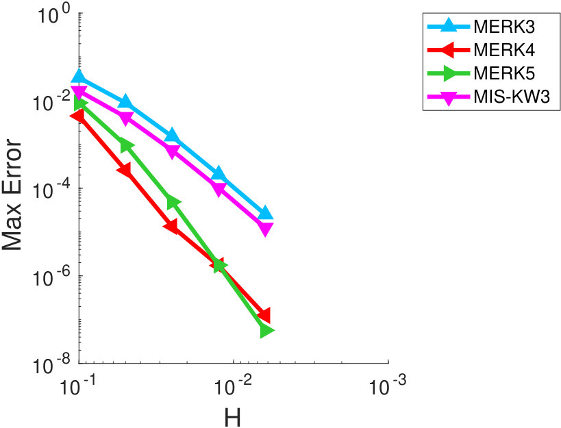 Figure 1
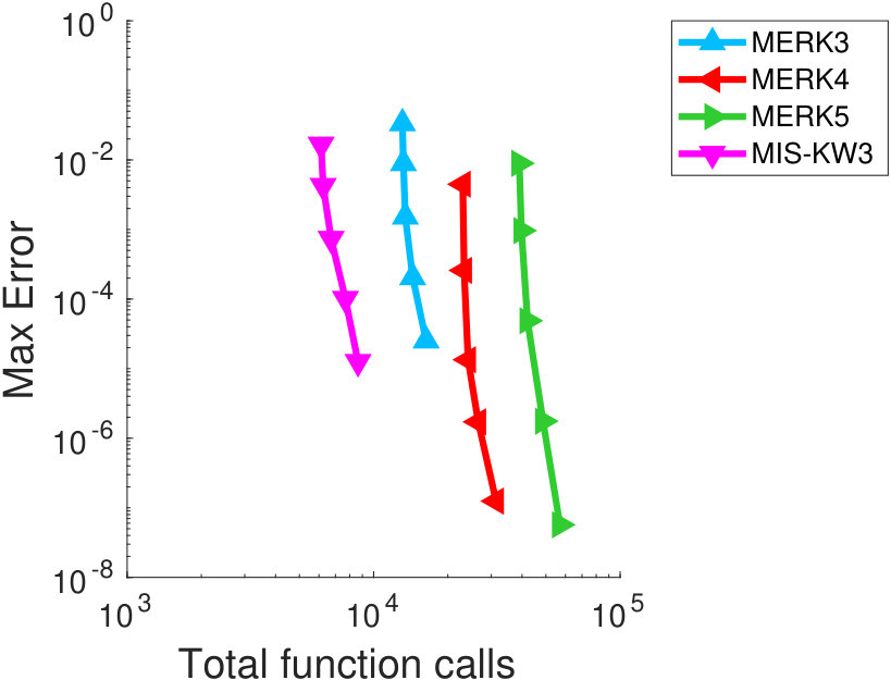 Figure 2
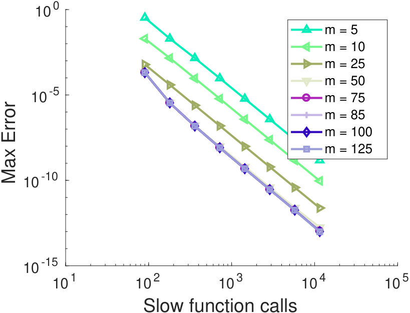 Figure 3
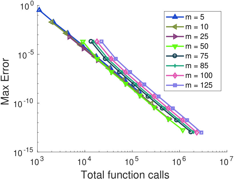 Figure 4
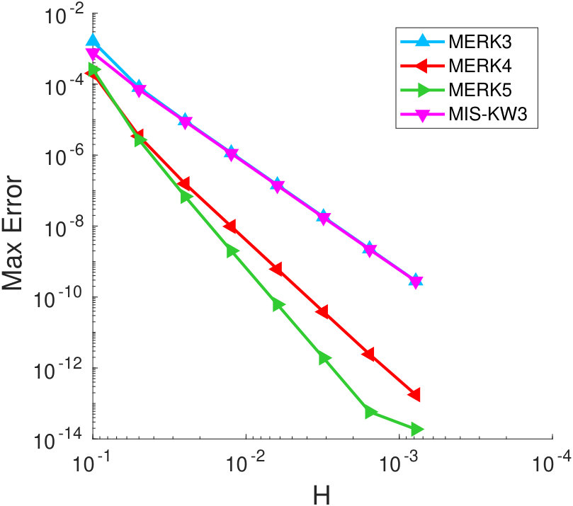 Figure 5
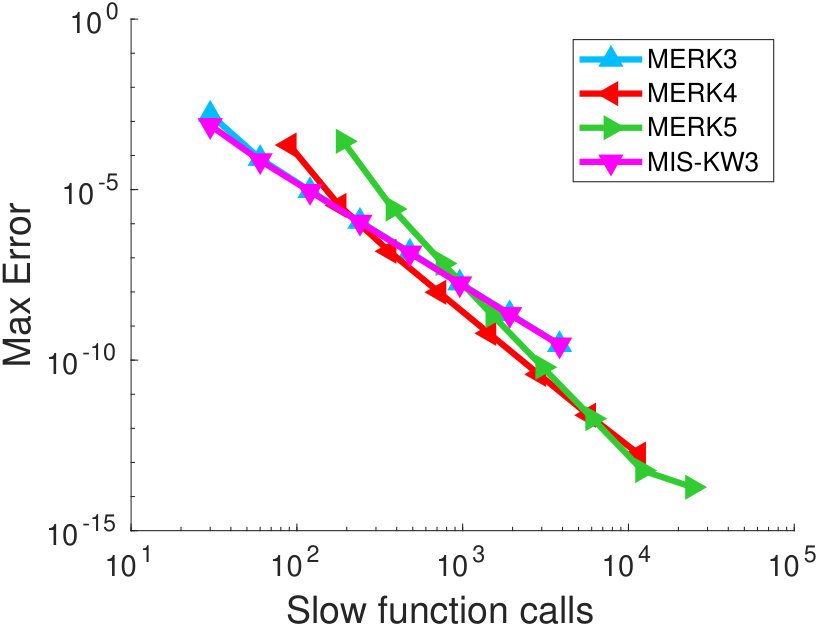 Figure 6
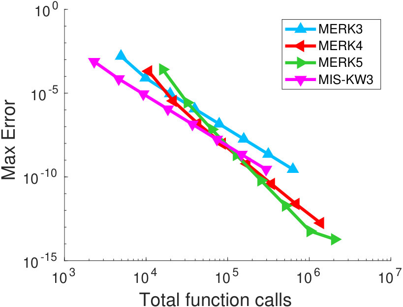 Figure 7
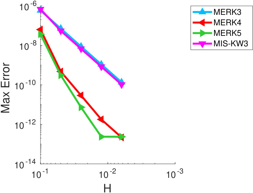 Figure 8
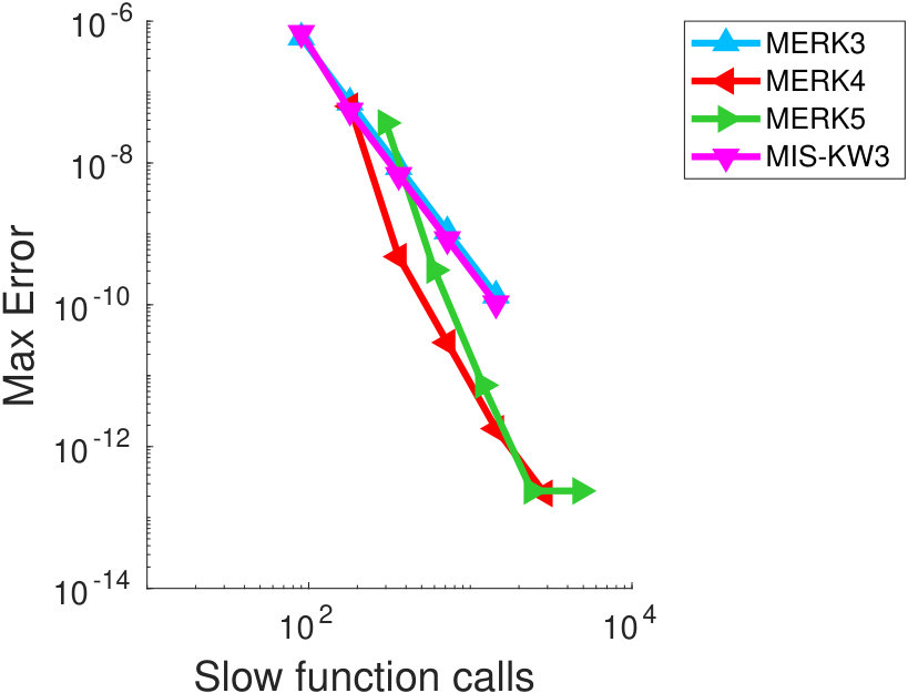 Figure 9
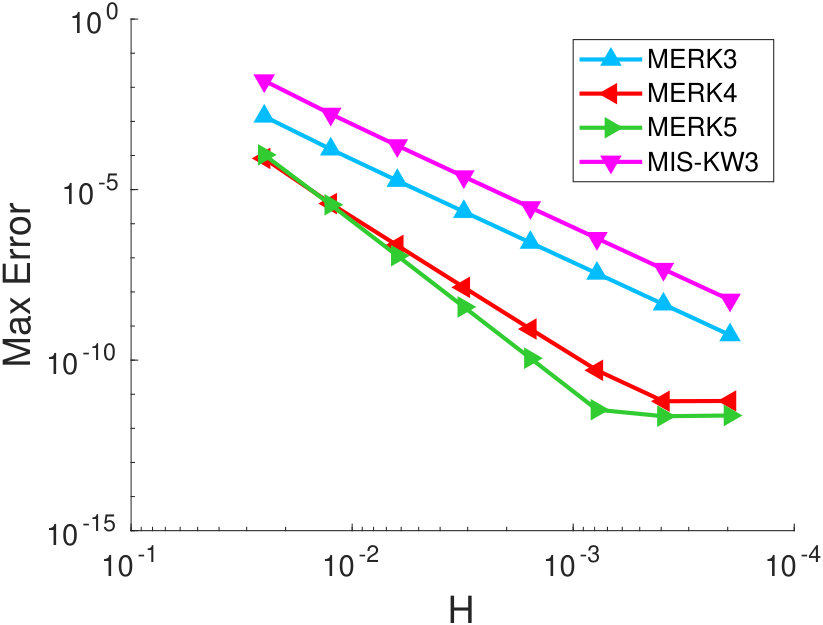 Figure 10
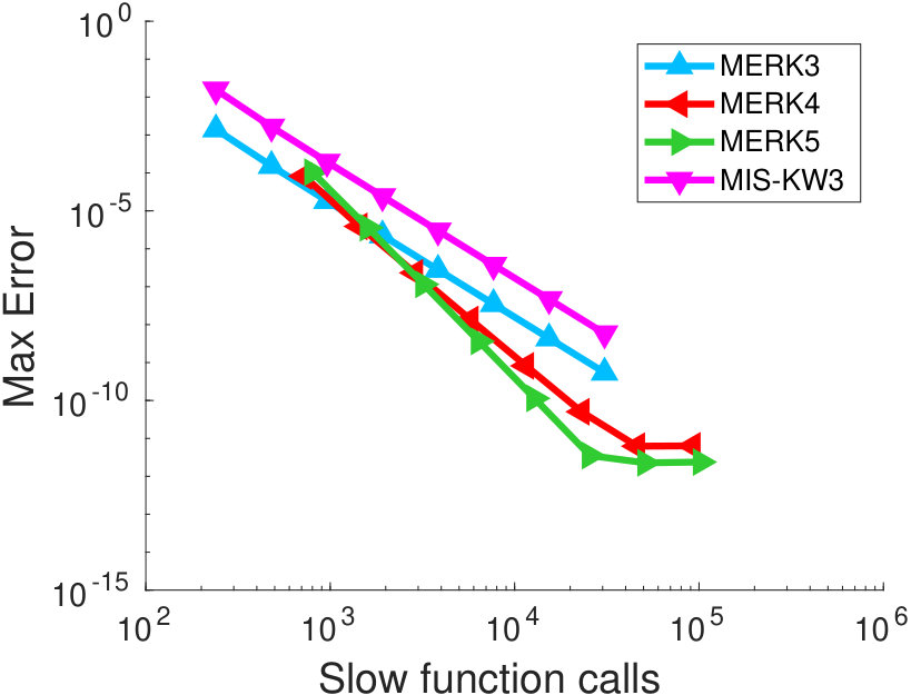 Figure 11
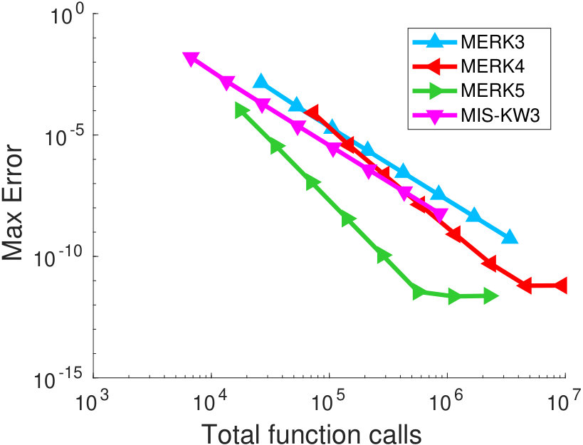 Figure 12
| MERK3() | MERK4() | MERK5() | ||||||
| Observed order | Observed order | Observed order | ||||||
| 2 | 2 | 2.00 | 3 | 3 | 3.01 | 4 | 4 | 4.00 |
| 3 | 2 | 2.00 | 4 | 3 | 3.01 | 5 | 4 | 4.00 |
| 2 | 3 | 3.03 | 3 | 4 | 3.99 | 4 | 5 | 4.97 |
| 3 | 3 | 3.03 | 4 | 4 | 3.99 | 5 | 5 | 4.97 |
| 4 | 4 | 3.03 | 5 | 5 | 3.99 | 6 | 6 | 4.96 |
Peer Reviews
No public reviews on file for this paper yet. If you reviewed it on a platform where reviews are public (OpenReview, ICLR, NeurIPS, ICML), you can paste yours below so the community can read it here.
Code & Models
Videos
No videos yet. Explain this paper in a talk, walkthrough, or lecture? Add one.
\newsiamremark
remarkRemark \newsiamremarkhypothesisHypothesis
\newsiamthmclaimClaim \headersHigh-order methods for multirate differential equationsV. T. Luan, R. Chinomona, and D. R. Reynolds
A new class of high-order methods for multirate differential equations ††thanks: Submitted to the editors DATE.
\fundingThis work was supported in part by the U.S. Department of Energy, Office of Science, Office of Advanced Scientific Computing Research, Scientific Discovery through Advanced Computing (SciDAC) program through the FASTMath Institute under Lawrence Livermore National Laboratory Subcontract B626484.
Vu Thai Luan
Rujeko Chinomona
Daniel R. Reynolds Department of Mathematics, Southern Methodist University, Dallas, TX 75275-0156 (, , ). [email protected]
Abstract
This work focuses on the development of a new class of high-order accurate methods for multirate time integration of systems of ordinary differential equations. The proposed methods are based on a specific subset of explicit one-step exponential integrators. More precisely, starting from an explicit exponential Runge–Kutta method of the appropriate form, we derive a multirate algorithm to approximate the action of the matrix exponential through the definition of modified “fast” initial-value problems. These fast problems may be solved using any viable solver, enabling multirate simulations through use of a subcycled method. Due to this structure, we name these Multirate Exponential Runge–Kutta (MERK) methods. In addition to showing how MERK methods may be derived, we provide rigorous convergence analysis, showing that for an overall method of order , the fast problems corresponding to internal stages may be solved using a method of order , while the final fast problem corresponding to the time-evolved solution must use a method of order . Numerical simulations are then provided to demonstrate the convergence and efficiency of MERK methods with orders three through five on a series of multirate test problems.
keywords:
multirate time integration, multiple time stepping, exponential integrators, exponential Runge–Kutta methods,
{AMS}
65L06, 65M20, 65L20
1 Introduction
In this paper, we focus on the construction, analysis, and implementation of efficient, highly accurate, multirate time stepping algorithms, based on various classes of explicit one-step exponential integrators. These algorithms may be applied to initial value problems (IVPs) of the form
[TABLE]
on the interval , where the vector field can be decomposed into a linear part comprising the “fast” time scale, and a nonlinear part comprising the “slow” time scale. Such systems frequently result from so-called “multi-physics” simulations that couple separate physical processes together, or from the spatial semi-discretization of time-dependent partial differential equations (PDEs). Our primary interest in this paper lies in the case where the fast component is much less costly to compute than the slow component, thereby opening the door for methods that evolve each component with different time step sizes – so-called multirate (or multiple time-stepping, MTS) methods. This case is common in practice when using a non-uniform grid for the spatial semi-discretization of PDEs, or in parallel computations where the fast component is comprised of spatially-localized processes but the slow component requires communication across the parallel network.
In recent years, there has been renewed interest in the construction of multirate time integration methods for systems of ODEs. Generally, these efforts have focused on techniques to achieve orders of accuracy greater than two, since second-order methods may be obtained through simple interpolation between time scales. These recent approaches broadly fit into two categories: methods that attain higher-order through extrapolation of low-order methods [1, 4, 5], and methods that directly satisfy order conditions for partitioned and/or additive Runge–Kutta methods [9, 14, 15, 24, 25, 27, 37, 39, 41, 42, 43, 44, 45]. Of these, the latter category promises increased efficiency due to the need to traverse the time interval only once. However, only very recently have methods of this type been constructed that can achieve full fourth-order accuracy [37, 44], and we know of no previous methods having order five or higher.
Among numerical methods that use the same time step for all components of (1.1), exponential integrators have shown great promise in recent years [6, 18, 19, 20, 21, 22, 30, 31, 32, 34, 28, 35]. Most such methods require the approximation of products of matrix functions with vectors, i.e., , for and .
Inspired by recent results on local-time stepping methods for problems related to (1.1) [10, 11, 12, 13], and motivated by the idea in [23, Sect. 5.3] that establishes a multirate procedure for exponential multistep methods of Adams-type, here we derive multirate procedures for exponential one-step methods. Starting from an -stage explicit exponential Runge–Kutta (ExpRK) method applied to (1.1), we employ the idea of backward error analysis to define modified differential equations whose exact solutions coincide with the ExpRK internal stages. These modified differential equations may then be evolved using standard ODE solvers at the fast time scale. We name the resulting methods as Multirate Exponential Runge–Kutta (MERK) methods.
The ability to construct modified ODEs for each slow ExpRK stage is dependent on the form of the ExpRK method itself, and we identify these restrictions within this manuscript. Using this approach, we derive a general multirate algorithm (Algorithm 1) that can be interpreted as a particular implementation (without matrix functions) of explicit exponential Runge-Kutta methods. With this algorithm in hand, we perform a rigorous convergence analysis for the proposed MERK methods. We additionally construct MERK schemes with orders of accuracy three through five, based on some well-known ExpRK methods from the literature.
We note that the resulting methods show strong similarities to the MIS methods in [24, 25, 41, 42, 43, 45] and the follow-on RMIS methods [44] and MRI-GARK methods [37], in that the MERK algorithm requires the construction of a set of modified “fast” initial-value problems that must be solved to proceed between slow stages, and where these modifications take the form of polynomials based on “slow” function data. While these approaches indeed result in similar algorithmic structure, (R)MIS and MRI-GARK methods are based on partitioned and generalized-structure additive Runge–Kutta theory [38], and as such their derivation requires satisfaction of many more order conditions than MERK methods, particularly as the desired method order increases, to the end that no MIS method of order greater than three, and no RMIS or MRI-GARK methods of order greater than four, have ever been proposed. Additionally, to obtain an overall order method, all fast IVPs for (R)MIS and MRI-GARK methods must be solved to order , whereas the internal stages in MERK methods may use an order solver. Finally, both (R)MIS and the MRI-GARK methods require sorted abcissae , a requirement that is not present for MERK methods.
The outline of this paper is as follows: in Section 2, we derive the general class of exponential Runge-Kutta methods in a way that facilitates construction of MERK procedures. In Section 3, we then derive the general MERK algorithm for exponential Runge–Kutta methods, and provide a rigorous convergence analysis for these schemes. In Section 4, we derive specific MERK methods based on existing exponential Runge–Kutta methods. We present a variety of numerical examples in Section 5 to illustrate the efficiency of the new MERK schemes with order of accuracy up to five. The main contributions of this paper are Algorithm 1, convergence analysis for MERK methods (Theorem 3.7), and the proposed MERK schemes with order of accuracy up to five.
2 Motivation
We begin with a general derivation of exponential Runge–Kutta methods [20, 22], which motivates a multirate procedure for solving (1.1).
2.1 Exponential Runge–Kutta methods
When deriving ExpRK methods, it is crucial to represent the exact solution of (1.1) at time using the variation-of-constants formula,
[TABLE]
The integral in (2.1) is then approximated using a quadrature rule having nodes and weights (), which yields
[TABLE]
By applying (2.1) (with in place of ), the unknown intermediate values in (2.2) can be represented as
[TABLE]
Again, one can use another quadrature rule with the same nodes as before (to avoid the generation of new unknowns) and new weights to approximate the integrals in (2.3). This gives
[TABLE]
Now, denoting the approximations and , then from (2.2) and (2.4) one may obtain the so-called exponential Runge–Kutta methods
[TABLE]
The formula (2.5) is considered explicit when for all (thus and consequentially ). Throughout this paper we restrict our attention to explicit exponential Runge–Kutta methods, which can be reformulated as (see [31, 33]):
[TABLE]
where
[TABLE]
Here, the coefficients and are often linear combinations of the functions and , respectively, wherein are given by
[TABLE]
and satisfy the recurrence relations
[TABLE]
2.2 Adopting the idea of backward error analysis
Motivated by the idea of [23, Sect. 5.3], and recalling the equations (2.1) and (2.3), we note that and are the exact solutions of the differential equation
[TABLE]
evaluated at and , respectively. In other words, solving (2.10) exactly (by means of using the variation-of-constants formula) on the time intervals and shows that and . Unfortunately, explicit representations of these analytical solutions are generally impossible to find, since and are unknown values. This observation, however, suggests the use of backward error analysis (see, for instance [16, Chap. IX]).
Given an exponential Runge-Kutta method (2.5), we therefore search for modified differential equations of the form (2.10), such that their exact solutions at and coincide with the ExpRK approximations () and , respectively. We may then approximate solutions to these modified equations to compute our overall approximation of (1.1).
3 Multirate exponential Runge–Kutta methods
In this section, we construct a new multirate procedure based on approximation of ExpRK schemes; we call the resulting algorithms Multirate Exponential Runge-Kutta (MERK) methods. Following this derivation, we present a rigorous stability and convergence analysis.
3.1 Construction of modified differential equations
We begin with the construction of MERK methods, through definition of modified differential equations corresponding with the ExpRK stages () and solution .
Theorem 3.1**.**
Assuming that the coefficients and of an explicit exponential Runge–Kutta method (2.6) may be written as linear combinations
[TABLE]
for some positive integers and , and where the functions and are given in (2.8), then and are the exact solutions of the linear differential equations
[TABLE]
at the times and , respectively. Here and are polynomials in given by
[TABLE]
Proof 3.2**.**
By changing the integration variable to in (2.8), we obtain
[TABLE]
Substituting and into (3.4) and inserting the obtained results for and into (3.1) shows that
[TABLE]
Using the fact that and
[TABLE]
we can write (2.6) in an equivalent form,
[TABLE]
for . We now insert the integral form of in (3.6) (with and ) and (3.5) into (3.7) to get
[TABLE]
*with and as shown in (3.3). Clearly, these representations (variation-of-constant formulas) show the conclusion of Theorem 3.1. In particular, and . Thus one can consider (3.2) as modified differential equations with identical solutions as the ExpRK approximations to (2.10). *
We note that the idea of using an ODE to represent a linear combination of matrix-vector was also used in [36].
3.2 MERK methods and a multirate algorithm
Clearly, the polynomials
and in (3.3) are not given analytically since are unknowns; however, these polynomials can be numerically determined as follows. For simplicity, we illustrate our procedure by starting with and . In this case we know and , so one can solve the ODE (3.2a) on to get an approximation to , . Then replacing the unknown in (3.3b) by , we have
[TABLE]
where . Since , we may then solve the ODE (3.2b) on with in place of to obtain an approximation .
This general process may be extended to larger numbers of stages and for subsequent time steps . Approximating (with ), then for , we define the following perturbed linear ODEs over :
[TABLE]
with
[TABLE]
that provide the approximations
[TABLE]
With these in place, we then solve the linear ODE
[TABLE]
over , with
[TABLE]
to obtain the approximate time-step solutions,
[TABLE]
Since the above procedure uses a “macro” time step to integrate the slow process, and a “micro” time step to integrate the fast process (via solving the ODEs (3.9) and (3.12)), we call the resulting methods (3.9)-(3.11) Multirate Exponential Runge–Kutta (MERK) methods. By construction, these MERK methods offer several interesting features. They reduce the solution of nonlinear problems (1.1) to the solution of a sequence of linear differential equations (3.9) and (3.12), using very few evaluations of the nonlinear operator . Thus they can be more efficient for problems where the linear part is much less costly to compute than the nonlinear part. Additionally, they do not require the computation of matrix functions, as is the case with ExpRK methods. Moreover, these methods do not require a starting value procedure as in multirate algorithms for exponential multistep methods [7, 23].
We provide the following Algorithm 1 to give a succinct overview of the implementation of our MERK methods.
3.3 Stability and convergence analysis
Since MERK methods are constructed to approximate ExpRK methods, we perform their error analysis in the framework of analytic semigroups on a Banach space , under the following assumptions (see e.g., [21, 31]).
Assumption 1. The linear operator is the infinitesimal generator of an analytic semigroup on . This implies that
[TABLE]
and consequently , and are bounded operators.
Assumption 2 (for high-order methods). The solution of (1.1) is sufficiently smooth with derivatives in , and is sufficiently Fréchet differentiable in a strip along the exact solution. All derivatives occurring in the remainder of this section are therefore assumed to be uniformly bounded.
We analyze the error in MERK methods starting with the local error of ExpRK methods. Therefore, we first consider (2.5) (in its explicit form) with exact initial value, :
[TABLE]
and thus the MERK methods (3.2)–(3.3) are considered with polynomials
[TABLE]
where .
Error notation. Since MERK methods consist of approximations to approximations, we must clearly isolate the errors induced at each approximation level. To this end, we let denote the global error at time of a MERK method (3.9)-(3.11). Let denote the local error at of the base ExpRK method. Let and denote the (global) errors of the ODE solvers when integrating (3.9) on and (3.12) on (note that since ).
First, we may write total error as the sum of the errors in each approximation,
[TABLE]
Applying the variation-of-constants formula to (3.13) and using (3.5b), we then write
[TABLE]
Inserting and from (3.18) and (3.15b) into (3.17) gives
[TABLE]
where
[TABLE]
Next, we prove some preliminary results.
Lemma 3.3**.**
Denoting and , we have
[TABLE]
with
[TABLE]
Furthermore, under Assumption 2, the bound
[TABLE]
*is held as long as remains in a sufficiently small neighborhood of [math]. *
Proof 3.4**.**
We first rewrite
[TABLE]
Here is the exact solution of (3.9), which can be represented by the variation-of-constants formula and then rewritten by using (3.5a) and (3.10) as:
[TABLE]
Subtracting (3.15a) from (3.25) and inserting the obtained result into (3.24) gives
[TABLE]
Using the Taylor series expansion of at , we get
[TABLE]
*with the remainder given in (3.22), which clearly satisfies (3.23) due to Assumption 2. Inserting (3.27) into (3.26) shows (3.21). *
Lemma 3.5**.**
Under Assumptions 1 and 2, there exist bounded operators and on such that
[TABLE]
*Note that also depends on , , , (), and ; and also depends on , , , and . *
Proof 3.6**.**
Inserting (3.27) (with in place of ) into (3.20) gives
[TABLE]
Using the recursion (3.21) from Lemma 3.3, we further expand as
[TABLE]
*Using (3.21) and (3.23) () and proceeding by induction, one can complete the recursion (3.30) for . Inserting this recursion into (3.29) (and noting that ) yields (3.28). Based on the structure of (3.30) and (3.29), under the given assumptions it is clear that the boundedness of and follow from the boundedness of , , and . *
We now present the main convergence result for MERK methods.
Theorem 3.7**.**
Let the initial value problem (1.1) satisfy Assumptions 1–2. Consider for its numerical solution a MERK method (3.9)–(3.11) that is constructed from an ExpRK method of global order . We further assume that the “fast” ODEs (3.9) and (3.12) associated with the MERK method are integrated with micro time step by using ODE solvers that have global order of convergence and , respectively, and where is the number of fast steps per slow step. Then, the MERK method is convergent, and has error bound
[TABLE]
*on compact time intervals . Here, the constant depends on , but is independent of and ; and the constants and also depend on the error constants of the choosen ODE solvers. *
Proof 3.8**.**
We first note that since we only employ the fast ODE solvers on time intervals and , then our assumption regarding their accuracies of order and is typically equivalent to [17, Thm. 3.6]
[TABLE]
(due to (3.6)) where are the Lipschitz constants for the increment functions of the ODE solvers applied to the problems (3.9) and (3.12), respectively.
*For simplicity of notation, we denote .
Clearly, is a bounded operator and thus (3.28) becomes*
[TABLE]
Inserting this into (3.19) gives
[TABLE]
Solving recursion (3.34) and using (since ) finally yields
[TABLE]
Since the ExpRK method has global order , we have the local error , and from (3.32) we have , . Using (3.14) we derive from (3.35) that
[TABLE]
*An application of a discrete Gronwall lemma to (3.36) results in the bound (3.31). *
Remark 3.9**.**
*Since , Theorem 3.7 implies that for a MERK method (3.9)–(3.11) to converge with order , the inner ODE solvers for (3.9) and (3.12) must have orders and , respectively. *
4 Derivation of MERK methods
Based on the theory presented in Section 3, we now derive MERK schemes up to order 5, relying heavily on ExpRK schemes that fit the assumption of Theorem 3.1. As we are interested in problems with significant time scale separation , we primarily focus on stiffly-accurate ExpRK schemes. Since MERK methods involve linear ODEs (3.9) and (3.12) with a fixed coefficient matrix for the fast portion, they are characterized by the polynomials defined in (3.10) and (3.13). Therefore, when deriving MERK schemes we display only their corresponding polynomials and .
4.1 Second-order methods
When searching for stiffly-accurate second-order ExpRK methods, we find the following scheme that uses stages (see [20, Sect. 5.1]) and satisfies Theorem 3.1:
[TABLE]
From this, using the conclusion of Theorem 3.1, we derive the corresponding family of second-order MERK methods, which we call MERK2:
[TABLE]
Since we do not use this scheme in our numerical experiments, we do not specify a value for . We note that for these methods, the fast time scale must be evolved a duration of for each slow time step.
4.2 Third-order methods
Also from [20, Sect. 5.2] we consider the following family of third-order, three-stage, ExpRK methods that satisfy Theorem 3.1:
[TABLE]
From these, we construct the following third-order MERK3 scheme:
[TABLE]
In our numerical experiments with this scheme, we choose . Hence, the fast time scale must be evolved a duration of for each slow time step.
4.3 Fourth-order methods
To the best of our knowledge, the only 5 stage, stiffly-accurate ExpRK method of order four was given in [20, Sect. 5.3]. However, this scheme does not satisfy Theorem 3.1 due to the coefficient
[TABLE]
which is not a linear combination of . Therefore, we cannot use it to derive a fourth-order MERK scheme. However, in a very recent submitted paper [29], we have derived a family of fourth-order, 6-stage, stiffly-accurate ExpRK methods (named expRK4s6), that additionally fulfill Theorem 3.1:
[TABLE]
Since the pairs of internal stages and are independent of one other (they can be computed simultaneously) and have the same format, this scheme behaves like a 4-stage method. Hence, instead of using 6 polynomials we need only 4 to derive the following family of fourth-order MERK schemes, which we call MERK4:
[TABLE]
For our numerical experiments, we choose the coefficients , , and . With this choice, we may then solve the linear ODE (3.9) using the polynomial on to get both and (since ) without solving an additional fast differential equation on . Similarly, we may solve the linear ODE (3.9) with the polynomial on to obtain both and . As a result, the fast time scale must only be evolved for a total duration of for each slow time step.
4.4 Fifth-order methods
Simiar to fourth-order ExpRK methods, there are no stiffly-accurate fifth-order methods available in the literature that fulfill Theorem 3.1. In particular, the only existing fifth-order scheme (expRK5s8, that requires 8 stages) was constructed in [31]. However, its coefficients , , , and involve several different linear combinations of with different scalings , and may not be used to create a MERK method. Again, in [29], we have constructed a new family of efficient, fifth-order, 10-stage, stiffly-accurate ExpRK methods (called expRK5s10) that fulfills Theorem 3.1:
[TABLE]
Although this scheme has 10 stages, again its structure facilitates an efficient implementation. Specifically, we note that there are multiple stages which share the same format (same matrix functions with different inputs ), and are independent of one another (namely, , , and ). These groups of stages can again be computed simultaneously, allowing the scheme to behave like a 5-stage method. We therefore propose the corresponding fifth-order MERK methods that use only 5 polynomials, which we name MERK5:
[TABLE]
For our numerical experiments, we choose , , , , and . Again, since , when solving the fast time-scale problem (3.9) with polynomial on gives and . Similarly, since , , and can be obtained by solving a single fast time-scale problem with polynomial on . Finally since , one can compute , , and by solving a single fast time-scale problem with polynomial on . The sum total of these solves corresponds to evolving the fast time scale for an overall duration of for each slow time step.
5 Numerical experiments
In this section we present results from a variety of numerical tests to examine the performance of the proposed MERK3, MERK4 and MERK5 methods. These tests are designed to confirm the theoretical convergence rates from Section 3.3, and compare efficiency against the Multirate Infinitesimal Step method MIS-KW3, which uses a similar approach of evolving the fast component using modified systems of differential equations [26, 45, 41, 43]. Unless otherwise noted, we run these methods with inner explicit Runge-Kutta ODE solvers of the same order of convergence as the MERK method, :
- •
Third order MIS-KW3 uses the Knoth-Wolke-ERK inner method [26];
- •
Third order MERK3 uses the ERK-3-3 inner method, \begin{array}[]{c|ccc}0&&&\\ 1/2&1/2&&\\ 1&-1&2&\\ \hline\cr&1/6&2/3&1/6\end{array};
- •
Fourth order MERK4 uses the ERK-4-4 inner method [17, Table 1.2, left];
- •
Fifth order MERK5 uses the Cash-Karp-ERK inner method [2].
We note that although Theorem 3.7 guarantees that when using a MERK method of order , the internal stage solutions (3.9) can be computed with a solver of order and the step solution (3.12) can use a solver of order , for simplicity we have used in the majority of our tests. However, we more closely investigate these inner solver order requirements in Section 5.3 below.
Not all of our test problems have convenient analytical solutions; for these tests, we compute a reference solution using an 8th order explicit or a 12th order implicit Runge-Kutta method with a time step smaller than the smallest micro time step . When computing solution error, we report the maximum absolute error over all time steps and solution components. From these, we compute convergence rates using a linear least-squares fit of the log-error versus log-macro time step . For each test we present three types of plots: one convergence plot (error vs ) and two efficiency plots. Generally, efficiency plots present error versus the computational cost. However in the multirate context, fast and slow function costs can differ dramatically. As such, we separately consider efficiency using total function calls and slow function calls. Since the dominant number of total calls are from the fast function, the “total” plots represent the method efficiency for simulations with comparable fast/slow function cost, whereas the “slow-only” plots represent the method efficiency for simulations in which the slow function calls are significantly more expensive (as explained in Section 1 as our original motivation for multirate methods). Individual applications will obviously lie somewhere between these extremes, but we assume that they are typically closer to the “slow-only” results.
Applications scientists traditionally use multirate solvers for one of two reasons. The first category are concerned with simulations of stiff systems, but where they choose to use a subcycled explicit method instead an implicit one for the stiff portion of the problem. Generally, these applications are primarily concerned with selecting to satisfy stability of the fast time scale (instead of accuracy). The second category consider simulations wherein it is essential to capture the coupling between the slow and fast times scales accurately, since temporal errors at the fast time scale can significantly deteriorate the slow time scale solution; here is chosen based on accuracy considerations. We therefore separately explore test problems in both of these categories in the Sections 5.1 and 5.2 below.
To facilitate reproducibility of the results in this section, we have provided an open-source MATLAB implementation of the MERK3, MERK4, MERK5 and MIS-KW3 methods, along with scripts to perform all tests from this section [3].
5.1 Category I
As this category of problems is concerned with stability at the fast time scale, we choose a fixed, linearly stable micro time step , and vary the macro time step (and similarly, ). To this end, we focus on two stiff applications: a reaction diffusion problem and the brusselator problem.
5.1.1 Reaction Diffusion
We consider a reaction diffusion problem with a traveling wave solution similar to the one considered by Savcenco et al. [40],
[TABLE]
where . We discretize in space using a second order accurate central finite difference scheme using spatial points. This gives us a system for which we take and to be the discretized versions of and respectively. The micro time step is chosen to satisfy the Courant-Friedrichs-Lewy (CFL) linear stability condition, .
In the left of Figure 1 we plot the method convergence as is varied, which shows slighty convergence rates that are better than predicted for all methods tested. As this behavior is not consistently observed for the remaining test problems, we believe that this is an artifact of this particular test problem. Here, we compute the best-fit rates using only the error values larger than , where the error stagnates due to the accuracy of the reference solution.
The efficiency plots for both test problems in this category are very similar, so we present the “slow-only” efficiency plot for this problem in the right of Figure 1, saving the “total” efficiency plot for the next test. Here, we note that for tolerances larger than , MERK3 and MIS-KW3 are the most efficient, but for tighter tolerances MERK4 is the best. Although MERK5 has a higher rate of convergence, the increased cost per step causes it to lag behind until it reaches the reference solution accuracy, where it begins to overtake MERK4.
5.1.2 Brusselator
The brusselator is an oscillating chemical reaction problem for which one of the reaction products acts as a catalyst. It is widely used as a test for ODE solvers, including IMEX and multirate methods. We use a variant of this stiff nonlinear ODE system given by:
[TABLE]
over the interval , with parameters and . We convert this to have the multirate form (1.1) by defining
[TABLE]
In the left of Figure 2 we plot the error versus , and list the corresponding best-fit convergence rates. We observe that all the tested methods perform slightly worse than their predicted convergence rates, which we attribute to order reduction due to the stiffness of the problem; however, the relative convergence rates of each method compare as expected against one another.
For this test problem, we plot the efficiency based on total function calls in the right of Figure 2. We note that each curve is almost vertical since the micro time step is held constant for these tests, and is significantly smaller than . Here, MIS-KW3 takes the least amount of total function calls since its structure ensures that it only traverses the time step interval once when evaluating the modified ODEs, whereas MERK3, MERK4 and MERK5 require approximately 2, 3 and 3 traversals, respectively. We note that although these additional traversals of the time step interval result in significant increases in the number of fast function calls, the number of potentially more costly slow function calls for all methods is equal to the number of slow stages.
5.2 Category II
Recalling that our second category of multirate applications focuses on accurately coupling the fast and slow processes, for these test problems we choose a fixed time scale separation factor for each method/test, and vary (and proportionally, ). For this group of tests we consider a linear multirate problem from Estep et al. [8] for which the fast variables are coupled into the slow equation (one-directional coupling) and a linear multirate problem of our own design where both the fast and slow variables are coupled (bi-directional coupling). Since the “optimal” value of for each multirate algorithm is problem-dependent, we describe our approach for determining this value in Section 5.2.1 below.
5.2.1 One-directional coupling
We consider a linear system of ODEs [8]:
[TABLE]
over the interval . This has analytical solution , , and . We convert this problem to multirate form (1.1) by decomposing it as:
[TABLE]
We first discuss our approach in determining the “optimal” time-scale separation factor . For illustration, we consider MERK4 on this problem; however, we apply this approach to all methods for both this test and the following bi-directional coupling test in Section 5.2.2. We begin by repeatedly solving the problem (5.1) using the multirate method with different factors . For each value of , we vary (and hence ). We then analyze the resulting “total” and “slow-only” efficiency plots for each fixed value, as shown in Figure 3.
We first note that both plots show a group of values with identical efficiency, along with other less efficient results. In Figure 3(a), the more efficient group is comprised of larger values, whereas in Figure 3(b) the more efficient group has smaller values. This is unsurprising, since increases in for a fixed correspond to decreases in , leading to accuracy improvements at the fast time scale alone. While this will results in increased total function calls, the number of slow function calls will remain fixed. We therefore define the “optimal” as the value where the fast and slow solution errors are balanced. Hence, in Figure 3(b) this corresponds to the largest that remains in the more efficient group, and in Figure 3(a) this corresponds to the smallest that remains in the more efficient group. Inspecting both plots in Figure 3, the optimal value for MERK4 on this problem is . Carrying out a similar process for the other methods on this problem, MERK3 has an optimal value of , MERK5 , and MIS-KW3 has an optimal value of .
Using these values, In Figure 4 we plot the convergence results for the four methods on this problem, confirming the analytical orders of convergence, with errors stagnating around due to accumulation of floating-point roundoff. While we find slightly better-than-expected convergence rates for the MERK methods, and only the expected rate for MIS-KW3, we do not draw conclusions regarding this behavior.
Similarly, in Figure 5 we plot both the “total” and “slow-only” efficiency of each method on the one-directional test problem. When measuring only slow function calls, both MIS-KW3 and MERK3 tie for errors larger than , MERK4 is the most efficient for errors between and and MERK5 is the most efficient at the tightest error values. When the fast function calls are given equal weight as the slow, however, MIS-KW3 is the most efficient at errors larger than , while MERK5 is the most efficient at tighter error thresholds.
5.2.2 Bi-directional coupling
Taking inspiration from the preceding one-directional test, we designed a problem with coupling between both the fast and slow components to further demonstrate the flexibility and robustness of MERK methods. To this end, we consider the following test problem
[TABLE]
over . Converting to multirate form (1.1), we set and as:
[TABLE]
While this is a linear test problem that may be solved using the matrix exponential, this solution is difficult to represent in closed-form, and so we use a reference solution for convenience. Using the previously-described approach for determining the optimal time-scale separation factor for each method on this problem, we have for MERK3 and MERK4, for MERK5 and for MIS-KW3.
In Figure 6 we plot the convergence rates of each method on this test problem, again confirming the analytical orders of convergence, with errors stagnating around due to the reference solution accuracy.
Similarly, in Figure 7 we plot both the “slow-only” and “total” efficiency plots for this problem. Here, when measuring only the slow function calls, the most efficient method is MERK3 at error thresholds above , and MERK5 for smaller error values. Strikingly, when considering the total number of function calls, the MERK5 is the most efficient at nearly all error thresholds. We note, however, that the optimal time-scale separation factor for MERK5 is for this problem, which results in reduced fast function calls per slow step, and hence an overal reduction in total function calls.
5.3 Variations in the fast method
We finish by demonstrating the effects of using inner methods with differing orders of accuracy. Here, we consider only the MERK methods, applied to the bi-directional coupling problem (5.2). Here, we vary the order of method applied for computing both the internal stage solutions (3.9), , and the step solution (3.12), . Recalling the convergence theory presented in Theorem 3.7, a MERK method of order should use inner methods of orders and . However, in these tests we apply other variations on orders to ascertain whether (a) the inner methods could have even lower order and still obtain overall order , or (b) use of higher-order inner methods can result in overall convergence higher than . We present the best-fit convergence rates for this ensemble of tests in Table 1.
These numerical results show that in fact the inner method order requirements presented in Theorem 3.7 are both necessary and sufficient, i.e., the least-expensive combination for attaining a MERK method of order is to compute stage solutions (3.9) using an inner method of order , and the time step solution (3.12) using an inner method of order . Furthermore, use of higher-order inner methods with orders does not result in overall order higher than , due to the first term in Theorem 3.7, that corresponds to the coupling between the fast and slow processes.
6 Conclusion
We propose a novel class of multirate methods constructed from explicit exponential Runge–Kutta methods, wherein the action of the matrix exponential is approximated via solution of “fast” initial value problems for each ExpRK stage. Algorithmically, these methods offer a number of desirable properties. Since these are created through defining a set of modified IVPs (like (R)MIS and MRI-GARK methods), MERK implementations have near complete freedom in evolving the problem at the fast time scale; however, unlike (R)MIS and MRI-GARK, MERK methods may utilize inner solvers of reduced accuracy for the internal stages. Additionally, since the MERK structure follows directly from ExpRK methods satisfying Theorem 3.1, derivation of high-order MERK methods, including versions supporting embeddings for temporal adaptivity, is much simpler than for alternate multirate frameworks. As a result, MERK methods constitute the first multirate algorithms of order five, without requiring deferred correction or extrapolation techniques. Furthermore, the proposed approach may be similarly applied to exponential Rosenbrock methods, allowing for problems where the fast time scale is nonlinear, although such methods are not considered in this work.
In addition to proposing the MERK class of multirate methods and providing rigorous analysis of their convergence, we provide numerical comparisons of the performance of multiple MERK and MIS methods on a variety of multirate test problems. Based on these experiments, we find that the MERK methods indeed exhibit their theoretical orders of convergence, including tests that clearly demonstrate our primary convergence result in Theorem 3.7. Furthermore, the proposed methods compare favorably against standard MIS multirate methods, particularly when increased accuracy is desired and for problems wherein the “slow” right-hand side function is significantly more costly than the “fast.”
This work may be extended in numerous ways. As alluded to above, extensions of these approaches to explicit exponential Rosenbrock methods are straightforward, and are already under investigation. Additionally, extensions to higher order will follow from related developments of higher-order exponential methods. Finally, we plan to investigate the use of embeddings at both the fast and slow time scales to perform temporal adaptivity in both and for efficient, tolerance-based calculations.
Acknowledgments
The first author would like to thank Prof. Hochbruck and Dr. Demirel for their fruitful discussions during his visit at the Karlsruhe Institute of Technology (KIT) in 2013 under the support of the DFG Research Training Group 1294 “Analysis, Simulation and Design of Nanotechnological Processes”.
The reference list from the paper itself. Each links out to its DOI / PubMed record.
- 1[1] E. L. Bouzarth and M. L. Minion , A multirate time integrator for regularized stokeslets , Journal of Computational Physics, 229 (2010), pp. 4208–4224, https://doi.org/10.1016/j.jcp.2010.02.006 . · doi ↗
- 2[2] J. R. Cash and A. H. Karp , A variable order Runge-Kutta method for initial value problems with rapidly varying right-hand sides , ACM Trans. Math. Softw., 16 (1990), pp. 201–222, https://doi.org/10.1145/79505.79507 . · doi ↗
- 3[3] R. Chinomona, D. R. Reynolds, and V. T. Luan , Multirate exponential Runge–Kutta methods (MERK) . https://github.com/rujekoc/merk_v 1 , 2019.
- 4[4] E. Constantinescu and A. Sandu , Extrapolated implicit-explicit time stepping , SIAM J. Sci. Comput., 31 (2010), pp. 4452–4477.
- 5[5] E. M. Constantinescu and A. Sandu , Extrapolated multirate methods for differential equations with multiple time scales , J. Sci. Comput., 56 (2013), pp. 28–44.
- 6[6] S. M. Cox and P. C. Matthews , Exponential time differencing for stiff systems , Journal of Computational Physics, 176 (2002), pp. 430–455.
- 7[7] A. Demirel, J. Niegemann, K. Busch, and M. Hochbruck , Efficient multiple time-stepping algorithms of higher order , Journal of Computational Physics, 285 (2015), pp. 133–148.
- 8[8] D. Estep, V. Ginting, and S. Tavener , A posteriori analysis of a multirate numerical method for ordinary differential equations , Computer Methods in Applied Mechanics and Engineering, 223–224 (2012), p. 10–27.
