L1-norm Tucker Tensor Decomposition
Dimitris G. Chachlakis, Ashley Prater-Bennette, and Panos P., Markopoulos

TL;DR
This paper introduces L1-Tucker, a robust tensor decomposition method based on L1-norm, with algorithms that resist heavy data corruption, improving analysis of multi-way data.
Contribution
It formulates L1-Tucker decomposition and proposes two algorithms, L1-HOSVD and L1-HOOI, with analysis of their complexity and convergence.
Findings
L1-Tucker performs comparably to standard Tucker on clean data.
L1-Tucker shows strong robustness against heavily corrupted data.
Algorithms are effective for tensor reconstruction and classification.
Abstract
Tucker decomposition is a common method for the analysis of multi-way/tensor data. Standard Tucker has been shown to be sensitive against heavy corruptions, due to its L2-norm-based formulation which places squared emphasis to peripheral entries. In this work, we explore L1-Tucker, an L1-norm based reformulation of standard Tucker decomposition. After formulating the problem, we present two algorithms for its solution, namely L1-norm Higher-Order Singular Value Decomposition (L1-HOSVD) and L1-norm Higher-Order Orthogonal Iterations (L1-HOOI). The presented algorithms are accompanied by complexity and convergence analysis. Our numerical studies on tensor reconstruction and classification corroborate that L1-Tucker, implemented by means of the proposed methods, attains similar performance to standard Tucker when the processed data are corruption-free, while it exhibits sturdy resistance…
Click any figure to enlarge with its caption.
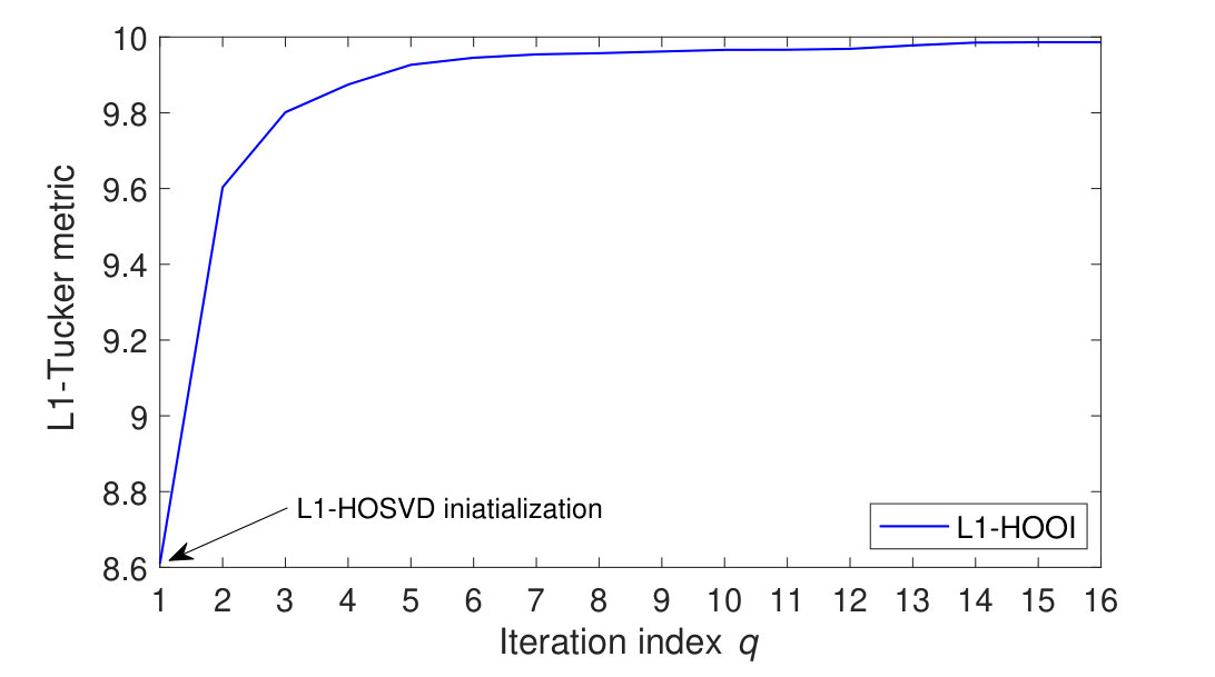 Figure 1
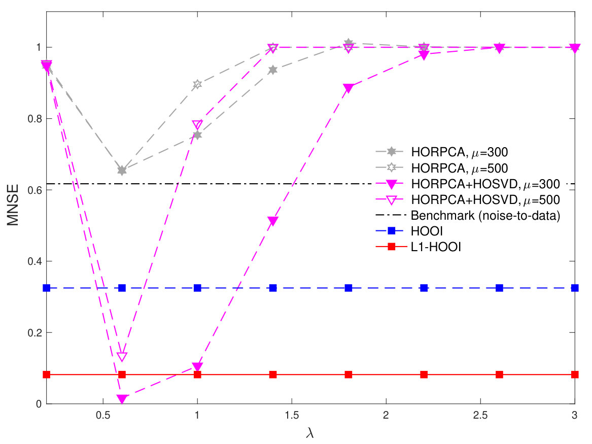 Figure 2
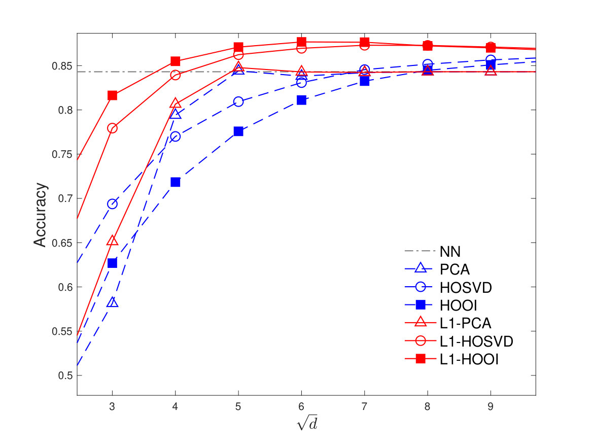 Figure 3
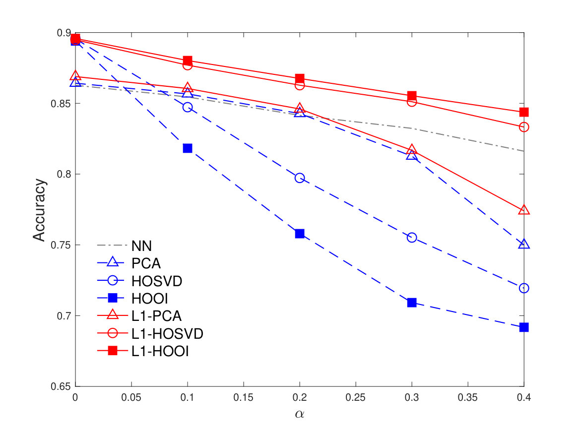 Figure 4
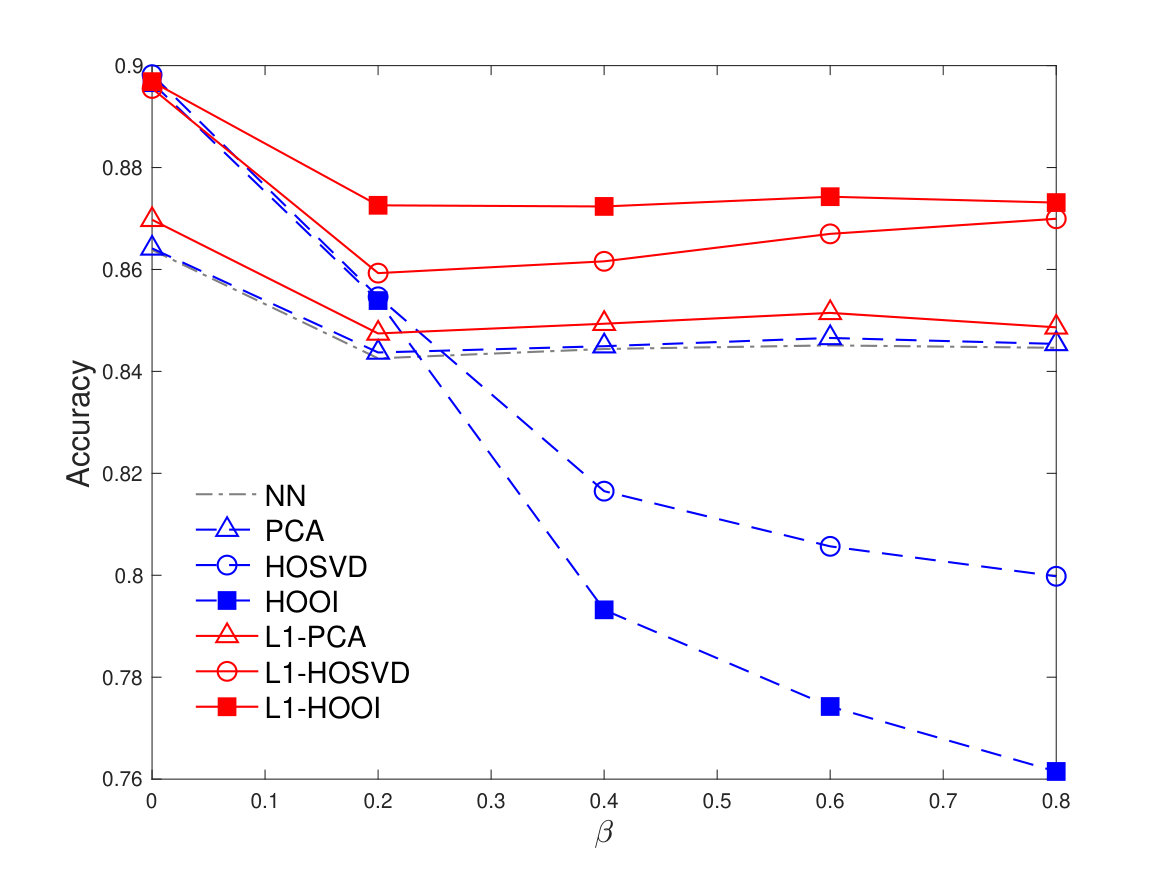 Figure 5
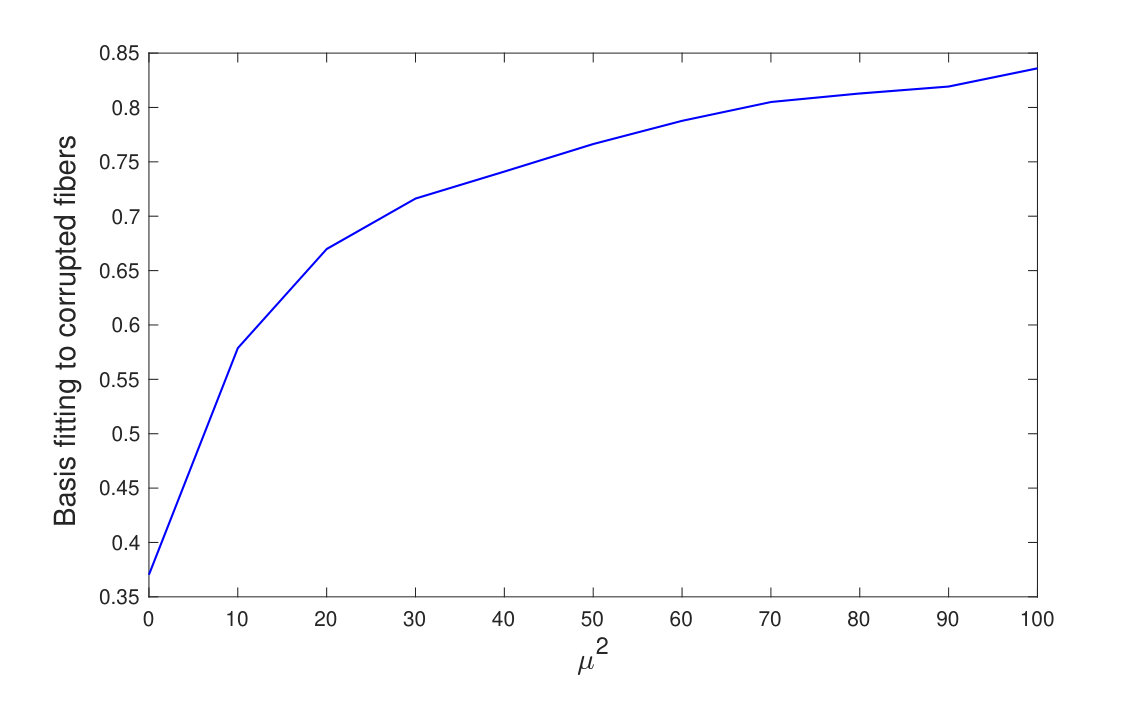 Figure 6
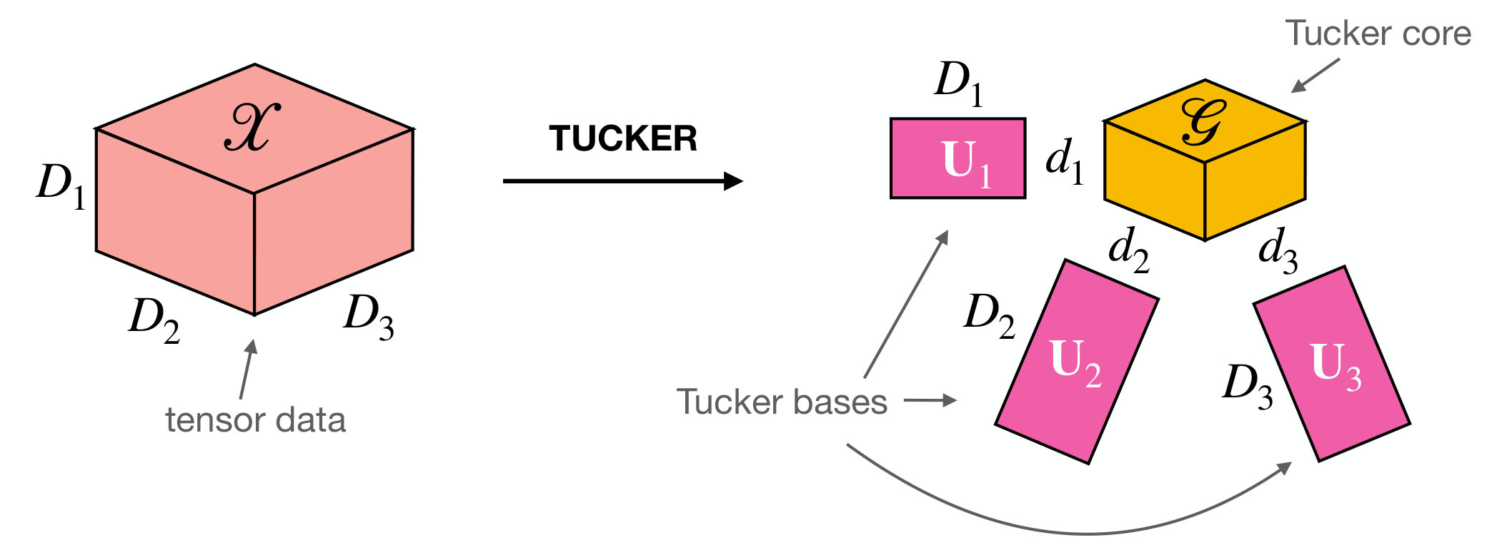 Figure 7
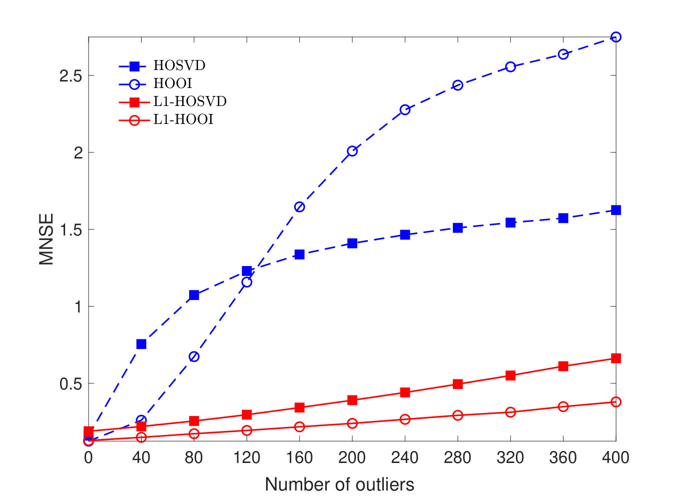 Figure 8
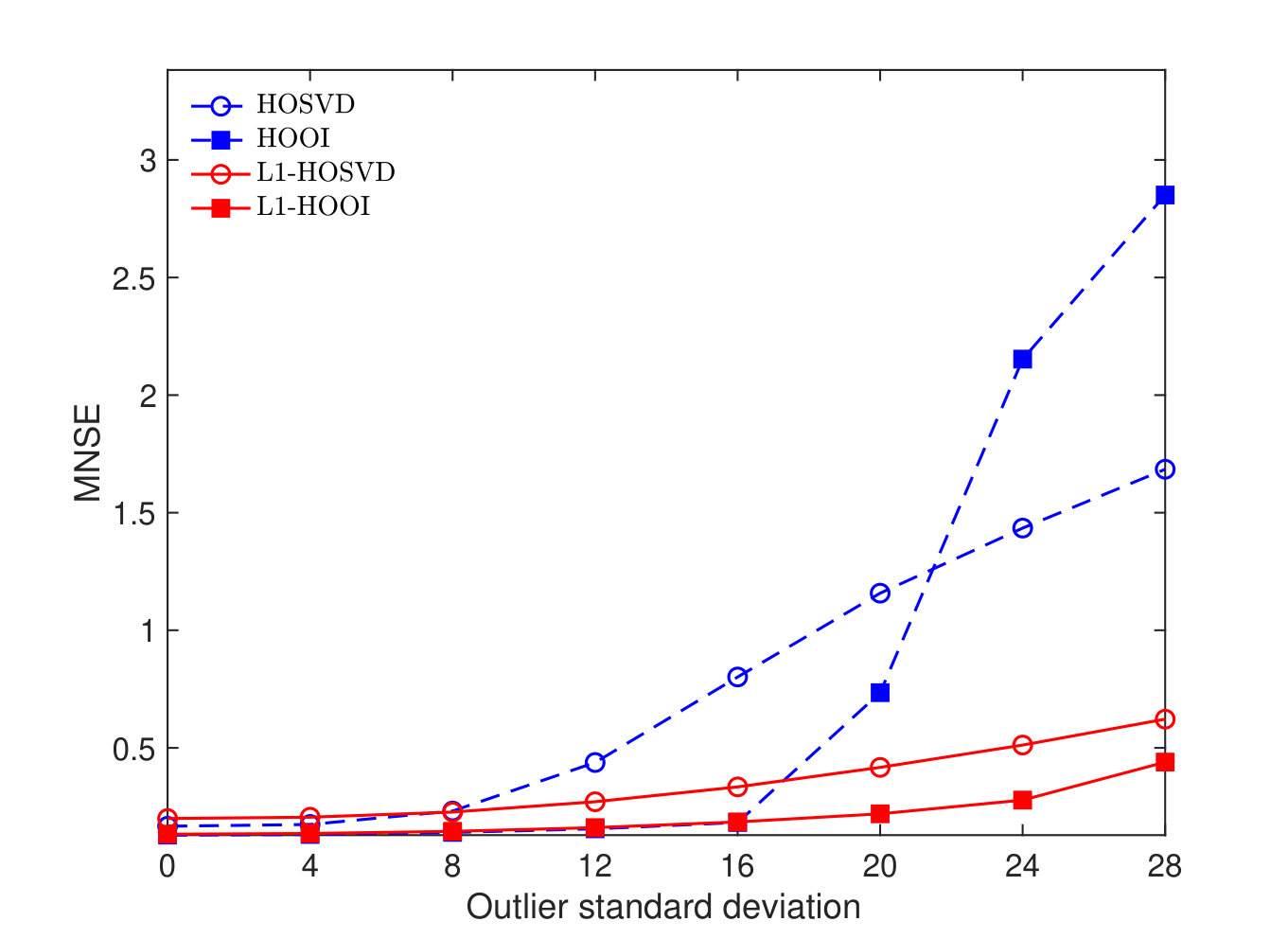 Figure 9
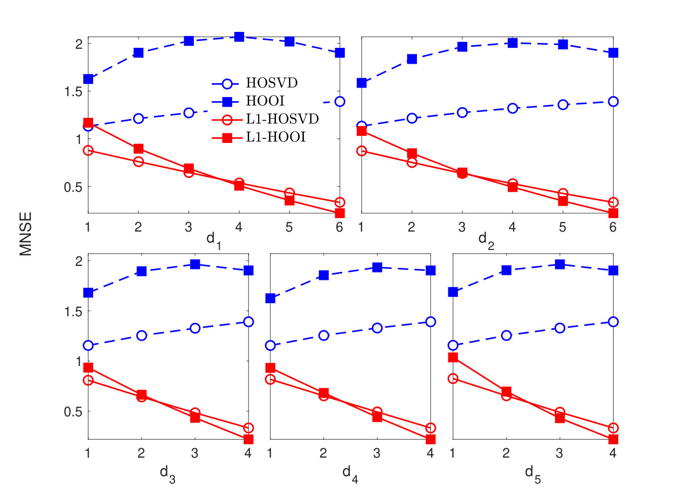 Figure 10
| Method | Cost |
|---|---|
| PCA (SVD) | |
| L1-PCA (AO) | |
| HOSVD | |
| L1-HOSVD | |
| HOOI | |
| L1-HOOI |
Peer Reviews
No public reviews on file for this paper yet. If you reviewed it on a platform where reviews are public (OpenReview, ICLR, NeurIPS, ICML), you can paste yours below so the community can read it here.
Videos
No videos yet. Explain this paper in a talk, walkthrough, or lecture? Add one.
L1-norm Tucker Tensor Decomposition
Dimitris G. Chachlakis,† Ashley Prater-Bennette,‡ and Panos P. Markopoulos*†∗* *†D. G. Chachlakis and P. P. Markopoulos are with the Department of Electrical and Microelectronic Engineering, Rochester Institute of Technology, Rochester, NY ([email protected], [email protected]).‡*A. Prater-Bennette is with the Air Force Research Laboratory, Information Directorate, Rome, NY ([email protected]).∗Corresponding author.This is a preprint of an article that has been submitted for peer-reviewed publication. This preprint may contain errata. Some preliminary results were presented in[1].
Abstract
Tucker decomposition is a common method for the analysis of multi-way/tensor data. Standard Tucker has been shown to be sensitive against heavy corruptions, due to its L2-norm-based formulation which places squared emphasis to peripheral entries. In this work, we explore L1-Tucker, an L1-norm based reformulation of standard Tucker decomposition. After formulating the problem, we present two algorithms for its solution, namely L1-norm Higher-Order Singular Value Decomposition (L1-HOSVD) and L1-norm Higher-Order Orthogonal Iterations (L1-HOOI). The presented algorithms are accompanied by complexity and convergence analysis. Our numerical studies on tensor reconstruction and classification corroborate that L1-Tucker, implemented by means of the proposed methods, attains similar performance to standard Tucker when the processed data are corruption-free, while it exhibits sturdy resistance against heavily corrupted entries.
Index Terms:
L1-norm, tensor decomposition, Tucker, corrupted data
I Introduction
Tucker decomposition [2, 3] is a cornerstone method for the analysis and compression of tensor data, with a wide array of applications in data science [4], signal processing, machine learning [5], and communications [6], among other fields. Tucker decomposition is typically computed by means of the Higher-Order Singular-Value Decomposition (HOSVD) algorithm, or the Higher-Order Orthogonal Iterations (HOOI) algorithm [7, 3]. Other popular variants include Truncated HOSVD (T-HOSVD) [7, 2, 8], Sequentially Truncated HOSVD (ST-HOSVD) [9], and Hierarchical HOSVD [10]. Parallel algorithms for HOSVD have also been developed [11], with the ability to process very large datasets. When an -way tensor is processed as a collection of -way tensor measurements, Tucker is reformulated to Tucker2 decomposition [12]. For the special case of , Tucker2 has also been presented as Generalized Low-Rank Approximation of Matrices (GLRAM) [13, 14] or 2-Dimensional Principal Component Analysis (2DPCA) [15, 16]. For , both Tucker and Tucker2 boil down to standard matrix Principal-Component Analysis (PCA), which is practically solved through Singular-Value Decomposition (SVD) [17]. In fact, both HOSVD and HOOI are high-order generalizations of SVD.
Due to its L2-norm formulation (minimization of the L2-norm of the residual-error or, equivalently, maximization of the L2-norm of the multi-way projection), standard Tucker decomposition has been shown to be sensitive against faulty entries within the processed tensor (also known as outliers), whether implemented by means of HOSVD, or HOOI[18, 19, 20]. The same sensitivity has also been documented in PCA, which is a special case of Tucker for -way tensors (matrices). For matrix decomposition, L1-norm-based PCA (L1-PCA) [21], formulated by simple substitution of the L2-norm in PCA with the L1-norm, has exhibited solid robustness against heavily corrupted data in an array of applications [22, 23, 24]. Similar outlier resistance has been recently attained by algorithms for L1-norm reformulation of Tucker2 decomposition of -way tensors (L1-Tucker2) [25, 26, 27, 20].
In this work we study L1-Tucker, an L1-norm reformulation of the general Tucker decomposition of -way tensors. Then, we propose two new algorithms for the solution of L1-Tucker, namely L1-HOSVD and L1-HOOI, accompanied by formal convergence and complexity analysis. Our numerical studies show that the proposed L1-Tucker methods perform similar to standard Tucker methods (HOSVD and HOOI) when the processed data are nominal. However, L1-HOSVD and L1-HOOI are markedly less affected by corruptions among the processed data.
II Technical Background
II-A Definitions and Notation
An -way tensor is an array of scalars, each entry of which is identified by indices. Vectors and matrices are -way and -way tensors, respectively. An -way tensor can also be viewed as an -way tensor in , for any , with for . For any fixed set of indices , vector is called a mode- fiber of . Thus, can also be viewed as a structured collection of its -th mode fibers, for any . Arranging all mode- fibers of tensor as columns of a matrix leads to a mode- matrix unfolding (also known as flattening) of , . Certainly, the mode- fibers of can be arranged in multiple different orders, resulting in column permutations of . In this work, we consider the common unfolding order, by which tensor element is mapped to the mode- unfolding element , for and , for every [3].
II-B Tucker Decomposition
Tucker tensor decomposition factorizes into orthonormal bases and a core tensor. Specifically, considering that satisfy , Tucker decomposition is formulated as
[TABLE]
where denotes the mode- tensor-to-matrix product [3], summarizes the multi-mode product , is the Stiefel manifold containing all rank- orthonormal bases in , and denotes the L2 (or Frobenius) norm, returning the summation of the squared entries of its tensor argument. If is the mode- basis derived by solving (1), then
[TABLE]
is the Tucker core of , and is Tucker-approximated by
[TABLE]
Equivalently, . If , it trivially holds that . The minimum values of for which are the respective mode ranks of . A schematic illustration of Tucker decomposition for is offered in Figure 1.
The solution to (1) is commonly pursued by means of the Higher-Order Singular-Value Decomposition algorithm (HOSVD) [7] or the Higher-Order Orthogonal Iterations algorithm (HOOI) [3]. A brief review of HOSVD and HOOI follows.
II-B1 HOSVD Method
HOSVD approximates , disjointly for each , by the principal components of the mode- unfolding ,
[TABLE]
computed by means of standard SVD. Arguably, HOSVD draws motivation from the case, where is a matrix and Tucker in (1) simplifies to maximizing . Indeed, for this special case of matrix decomposition, the optimal orthonormal factors can be found disjointly and coincide with the solution to (4), , where and . For the general case, however, all bases are to be found jointly and the HOSVD bases constitute, in general, approximations of the solution to (1).
II-B2 HOOI Method
HOOI is a converging iterative procedure, which provably attains a higher value of the metric in (1) than HOSVD, but still does not necessarily return the optimal solution [14, 28, 29, 30]. For each mode , HOOI is typically (but not necessarily) initialized to the solution of HOSVD as . Then, the HOOI algorithm conducts a sequence of provably converging iterations. That is, at the -th iteration, HOOI sets
[TABLE]
and updates
[TABLE]
obtained again by standard SVD of ( dominant left-singular vectors).
II-C Data Corruption and L1-norm Reformulation of PCA
Large datasets often contain heavily corrupted, outlying entries due to various causes, such as sensor malfunctions, errors in data storage/transfer, heavy-tail noise, intermittent variations of the sensing environment, and even intentional dataset “poisoning” [31]. Regretfully, such corruptions that lie far from the sought-after subspaces are known to significantly affect PCA and its multi-way generalization, Tucker, even when they appear as a small fraction of the processed data [21, 18, 20]. Accordingly, in such cases, the performance of any application that relies on PCA and Tucker can be compromised. This corruption sensitivity can be largely attributed to the L2-norm formulation of Tucker/PCA, which places squared emphasis on each entry of the core, thus benefiting corrupted fibers. To demonstrate this sensitivity of Tucker, we present the following simple example. We build with entries independently drawn from . Then, we corrupt additively the single entry with a point from . We apply HOSVD on to obtain the single dimensional bases , , and and measure the aggregate normalized fitting of the bases to the corrupted fibers as where , , and . We repeat this study times and plot in Figure 2 the average value of , versus . The impact of the single corrupted entry to the HOSVD bases (which tend to fit the corrupted fibers) is clearly documented.
To counteract the effect of data contaminations/corruptions, researchers have resorted in “robust” reformulations of PCA and Tucker. One popular approach seeks to approximate the processed data tensor as the summation of a sought-after low-rank component and a jointly optimized sparse component that models outlier corruption [32, 33, 19, 34]. This approach relies on ad hoc configured weights that regulate approximation rank, sparsity, and iteration step size. A rather more straightforward approach simply replaces the corruption-responsive L2-norm in PCA by the L1-norm. In matrix analysis, this modification resulted to the L1-PCA formulation [21], which constitutes a core component of the L1-Tucker framework proposed in this work. Therefore, for completeness, we briefly present below the theory behind L1-PCA, as well as a simple algorithm for its approximate computation.
Given a data matrix and , L1-PCA is defined as
[TABLE]
where the L1-norm returns the summation of the absolute entries of its matrix argument. L1-PCA in (7) was solved exactly in [21], where authors presented and leveraged the following Theorem 1.
Theorem 1**.**
Let be an optimal solution to
[TABLE]
Then, is an optimal solution to L1-PCA in (7). Moreover, [21].
Nuclear norm in (8) returns the sum of the singular values of its matrix argument. For any tall matrix that admits SVD , in Theorem 1 is defined as . Moreover, by the Procrustes Theorem [35], it holds that
[TABLE]
By means of the above Theorem 1, the solution to L1-PCA is obtained by the solution to (8), with an additional SVD step. (8) can be solved by exhaustive search in its finite-size feasibility set, or more intelligent algorithms of lower cost, as shown in [21]. Computationally efficient, approximate solvers for (8) and (7) were presented in [36, 37, 38, 39, 40]. Incremental solvers for L1-PCA were presented in [41, 42]. Algorithms for the complex-valued L1-PCA were recently presented in [43, 44]. To date, L1-PCA has found many applications in signal processing and machine learning, such as radar-based motion recognition and foreground-activity extraction in video sequences [23, 24]. Most recently, L1-PCA was extended to L1-norm-based Tucker2 formulation, specifically for -way tensors [26, 27].
Next, we briefly present the low-cost L1-PCA calculator of [37], based on alternating optimization, which will be employed as a module of our subsequent L1-Tucker decomposition developments. A pseudocode for this L1-PCA solver is offered in Algorithm 1. According to [21],
[TABLE]
By (9), for fixed , the middle part of (11) is maximized by . At the same time, for fixed , the middle part of (11) is maximized by , where returns the signs of the entries of its argument (). By the above observations, [37] pursued a solution to (7) in an alternating fashion, as
[TABLE]
and
[TABLE]
for , and arbitrary initialization . Omitting the explicit computation of the auxiliary matrix , (12)-(13) can take the compact form
[TABLE]
For completeness, we present below a proof of the monotonic metric increase attained by the above iterations.
Lemma 1**.**
For every ,
[TABLE]
At the same time, the metric of (7) is upper bounded by the exact L1-PCA solution [21]. Thus, the iteration in (14) is guaranteed to converge. In practice, iterations can be terminated when the metric-increase ratio
[TABLE]
drops below a predetermined threshold , or when exceeds a maximum number of permitted iterations. As shown in [37], the computational cost of the presented procedure is , where is the number of iterations. In practice, can be set to be linear in . Thus, the overall computational complexity of the above procedure is . In the sequel, we adopt the function notation to denote the basis returned upon termination/converge of the alternating optimization of (14).
III L1-Tucker Decomposition
III-A Formulation
Motivated by the corruption resistance of L1-PCA, in this work we study L1-Tucker decomposition. L1-Tucker derives by simply replacing the L2-norm in (1) by the sturdier L1-norm, as
[TABLE]
That is, (19) strives to maximize the sum of the absolute entries of the Tucker core –while standard Tucker maximizes the sum of the squared entries of the core. We note that, for any ,
[TABLE]
where . Thus, with respect to each individual basis, the metric of L1-Tucker resembles that of L1-PCA.
For , , and fixed , L1-Tucker in (19) simplifies to a special L1-Tucker2 decomposition, proposed and studied in [25, 27]. For the even more special case of , L1-Tucker2 was recently solved exactly in [20] through combinatorial optimization. For and fixed , L1-Tucker simplifies to L1-PCA, in the form of (7). The above works have shown that, even in its special cases, the exact solution to L1-Tucker is hard to find –which also holds true for standard Tucker decomposition.
Next, we present the first two approximate algorithms for solving the general L1-Tucker decomposition, in the form of (19).
III-B Proposed L1-HOSVD Method
We first present L1-HOSVD, an algorithm analogous to HOSVD for standard Tucker. Specifically, for every , L1-HOSVD seeks to optimize the mode- basis in (19) individually, by L1-PCA solution (exact or approximate) of the mode- matrix unfolding of , . That is, L1-HOSVD approximates the mode- basis in the solution of (19) by
[TABLE]
Similar to HOSVD, L1-HOSVD decouples the basis optimization task across the modes. We observe that (21) is, in fact, L1-PCA of the mode- flattening of . As mentioned above, there are multiple algorithms in the literature for solving L1-PCA in (21), both exactly and approximately [21, 36, 37]. As an L1-Tucker solution framework, L1-HOSVD allows for the employment of any solver for (21), thus making possible different performance/cost trade-offs. In this work, we demonstrate the employment of the simple alternating-optimization method of Algorithm 1, initialized, for example, at the solution of standard HOSVD. That is, L1-HOSVD returns
[TABLE]
for every . As presented in Section II-C, the computational cost of (22) is , where , when the number of L1-PCA iterations is linear in . A pseudocode of L1-HOSVD is offered in Algorithm 2.
III-C Proposed L1-HOOI Method
Similar to HOSVD, for general dense processed tensors, the disjoint mode optimization of L1-HOSVD may be very limiting. Next, we present L1-HOOI, an iterative algorithm for approximating the solution to (19). Specifically, L1-HOOI is arbitrarily initialized to feasible bases and conducts a sequence of iterations in which it updates all bases such that the objective value of L1-Tucker increases. Thus, when initialized to the L1-HOSVD bases, L1-HOOI is guaranteed to outperform L1-HOSVD in the L1-Tucker metric. In this approach, L1-HOSVD can be viewed as an initialization for L1-HOOI, or, conversely, L1-HOOI can be viewed as a refinement of L1-HOSVD.
Formally, L1-HOOI first initializes bases –for example, . Then, at the -th iteration, , it successively optimizes all bases, in increasing mode order . Specifically, at a given iteration and mode index , L1-HOOI fixes for and for and seeks the mode- basis that maximizes the L1-Tucker metric. That is, for a given index pair , L1-HOOI pursues
[TABLE]
Defining
[TABLE]
(23) is equivalently rewritten in the familiar L1-PCA form
[TABLE]
We notice that, in contrast to (21), the metric of (25) involves the jointly optimized bases of the other modes. As discussed above, there are multiple solvers for (25) that can attain different performance/cost trade-offs. The proposed L1-HOOI framework can be combined with any L1-PCA solver. In the sequel, we employ again the iterative solver of Algorithm 1. That is, for any (), we set
[TABLE]
A pseudocode of the proposed L1-HOOI method is offered in Algorithm 3. A formal convergence analysis of the L1-HOOI iterations is presented below.
III-C1 Convergence
We start with introducing Lemma 2, which shows that the -th update of the mode- basis increases the L1-Tucker metric.
Lemma 2**.**
Lemma 1 implies that, for fixed and ,
[TABLE]
We note that Lemma 2 would also hold if, instead of (26), we employed the bit-flipping iterative L1-PCA solver of [36], initialized to . Also, Lemma 2 certainly holds true if is computed by the exact solution of (25) –that is, by means of the exact algorithms of [21]. The following new Lemma 3 shows that, within the same iteration, the metric increases as we successively optimize the bases.
Lemma 3**.**
For any and every , it holds that
[TABLE]
Proof.
It holds that
[TABLE]
By induction, for every , . ∎
The following new Lemma 4 and Proposition 1 conclude our analysis on the monotonic increase of the L1-Tucker metric across the iterations of L1-HOOI.
Lemma 4**.**
For every , it holds that
[TABLE]
Proof.
It holds that
[TABLE]
∎
In view of Lemmas 2, 3, and 4, the following Proposition 1 holds true.
Proposition 1**.**
For any and every
[TABLE]
Proof.
It holds that
[TABLE]
∎
Denoting , the following Lemma 5 provides an upper bound for the L1-Tucker metric.
Lemma 5**.**
For any , it holds that
[TABLE]
Proof.
Let and define and . It holds that and . Also, define . We observe that
[TABLE]
Accordingly,
[TABLE]
∎
Lemma 5 shows that the L1-Tucker metric is upper bounded by . This, in conjunction with Proposition 1, imply that as increases the L1-HOOI iterations converge in the L1-Tucker metric.
To visualize the convergence, we carry out the following study. We form -way tensor , drawing independent entries from . Then, we apply L1-HOOI on , initialized to L1-HOSVD. In Fig. 3, we plot the evolution of L1-Tucker metric , versus the L1-HOOI iteration index . In accordance to our formal analysis, we observe the monotonic increase of the metric and convergence after iterations.
In practice, one can terminate the L1-HOOI iterations when the metric-increase ratio
[TABLE]
drops below a predetermined threshold , or when exceeds a maximum number of permitted iterations. Next, we discuss the computational cost of L1-HOOI.
III-C2 Complexity Analysis
As studied above, initialization of L1-HOOI by means of L1-HOSVD costs , where . Then, at iteration , L1-HOOI computes matrix in (25) and its L1-PCA, for every . Matrix can computed by a sequence of matrix-to-matrix products as follows. First, we compute the mode- product of with , for some ( if and if ), with cost . Next, we compute the -mode product of with , for some , with cost , where . We observe that the second product has lower cost than the first, for any selection of and . Similarly, each subsequent mode product will have further reduced cost. Thus, keeping the dominant term (cost of first product) and taking products in a computationally favorable order, the computation of costs . Importantly, the cost of computing is the same for every iteration index . After is computed, (25) is solved with cost , as shown above, where . Thus, for fixed , computation and L1-PCA of cost . Then, we observe that, there exists mode index such that, the cost of computing and its L1-PCA basis dominates over the respective cost of the -mode for every . The latter implies that the dominant cost at iteration of L1-HOOI is . Denoting by the maximum number of iterations permitted by L1-HOOI, the overall computational cost of L1-HOOI is . In Table I, we offer the computational costs of PCA, L1-PCA, HOSVD, L1-HOSVD, HOOI, and L1-HOOI. We observe that the costs of the proposed L1-HOSVD and L1-HOOI algorithms are comparable with those of standard HOSVD and HOOI respectively. Next, we conduct numerical studies and compare the performance of standard Tucker solvers with that of the proposed L1-Tucker algorithms.
IV Numerical Studies
IV-A Tensor Reconstruction
We set , , , , , and generate Tucker-structured . The core tensor draws entries from and, for every , is an arbitrary basis. We corrupt all entries of with zero-mean unit-variance additive white Gaussian noise (AWGN), disrupting its Tucker structure. Moreover, we corrupt out of the entries of –corruption ratio – by adding high magnitude outliers drawn from . Thus, we form , where and model AWGN and sparse outliers, respectively. Our objective is to reconstruct from the available . Towards our objective, we Tucker decompose by means of HOSVD, HOOI, L1-HOSVD, and L1-HOOI and obtain bases . Then, we reconstruct as . The normalized squared error (NSE) is defined as In Figure 4(a), we set () and plot the mean NSE (MNSE), evaluated over 1000 independent noise/outlier realizations, versus outlier standard deviation . In the absence of outliers (), all methods under comparison exhibit similarly low MNSE. As the outlier standard deviation increases the MNSE of all methods increases. We notice that the performances of HOSVD and HOOI markedly deteriorate for and respectively. On the other hand, L1-HOSVD and L1-HOOI remain robust against corruption, across the board.
In Figure 4(b), we set and plot the MNSE versus number of outliers . Expectedly, in the absence of outliers (), all methods exhibit low MNSE. As the number of outliers increases, HOSVD and HOOI start exhibiting high reconstruction error, while L1-HOSVD and L1-HOOI remain robust. For instance, the MNSE of L1-HOSVD for outliers is lower than the MNSE of standard HOSVD for (ten times fewer) outliers.
Finally, in Figure 4(c), we set , ( of total data entries are corrupted) and plot the MNSE versus while is set to its nominal value for every . We observe that, even for a very small fraction of outlier corrupted entries in , standard Tucker methods are clearly misled across all modes. On the other hand, the proposed L1-Tucker counterparts, exhibit sturdy outlier resistance and reconstruct well, remaining almost unaffected by the outlying entries in .
A robust tensor analysis algorithm, specifically designed for counteracting sparse outliers, is the High-Order Robust PCA (HORPCA) [19]. Formally, given , HORPCA solves
[TABLE]
Authors in [19] presented the HoRPCA-S algorithm for the solution of (48) which relies on a specific sparsity penalty parameter , as well as a thresholding variable . The model in (48) was introduced considering that, apart from the sparse outliers, there is no dense (full rank) corruption to (see [19], Section 2.6). In the case of additional dense corruption, HORPCA is typically accompanied by HOSVD [19, 34, 33]. In the sequel, we refer to this approach as HORPCA+HOSVD.
In our next study, we set , , and for every , and build the Tucker-structured data tensor , where the entries of core are independently drawn from . Then, we add both dense AWGN and sparse outliers, creating , where the entries of noise are drawn independently from and the non-zero entries of (in arbitrary locations) are drawn from . Then, we attempt to reconstruct from the available using HOOI, HORPCA (for and ), HORPCA+HOSVD (same and combinations as HORPCA), and the proposed L1-HOOI.
In Figure 5, we plot MNSE computed over data/noise/corruption realizations, versus for the four methods. In addition, we plot the average noise-to-data benchmark In accordance with our previous studies, we observe that L1-HOOI offers markedly lower MNSE than standard HOOI. In addition, we notice that for specific selection of and ( and ) HORPCA+HOSVD may attain MNSE even lower than HOOI. However, for any different selection of , HORPCA+HOSVD attains higher MNSE than HOOI. In addition, we plot the performance of HORPCA when it is not followed by HOSVD. We notice that, expectedly, for specific selections of and the method is capable of removing the outliers, but not the dense noise component –thus, the MNSE approaches the average noise-to-data benchmark. This study highlights the corruption-resistance of L1-HOOI, while, similarly to HOSVD and HOOI, it does not depend on any tunable parameters, other than .
IV-B Classification
Tucker decomposition is commonly employed for classification of multi-way data samples. Below, we consider the Tucker-based classification framework originally presented in [45]. That is, we consider classes of order- tensor objects of size and labeled samples available from the -th class, , that can be used for training a classifier. The training data from class are organized in tensor and the total of training data are organized in tensor , constructed by concatenation of across mode .
In the first processing step, is Tucker decomposed, obtaining the feature bases for the first modes (feature modes) and the sample basis for the -th mode (sample mode). The obtained feature bases are then used to compress the training data, as
[TABLE]
for every . Then, the compressed tensor objects from the -th class are vectorized (equivalent to mode- flattening) and stored in the data matrix
[TABLE]
where . Finally, the labeled columns of are used to train any standard vector-based classifier, such as support vector machines (SVM), or -nearest-neighbors (-NN).
When an unlabeled testing point is received, it is first compressed using the Tucker-trained bases as . Then, is vectorized as . Finally, vector is classified based on the standard vector classifier trained above.
In this study, we focus on the classification of order- data () from the MNIST image dataset of handwritten digits [46]. Specifically, we consider digit classes (digits ) and image samples of size available from each class. To make the classification task more challenging, we consider that each training image is corrupted by heavy-tail noise with probability . Then, each pixel of a corrupted image is additively corrupted by heavy tailed noise , with probability . Denoting the average pixel energy by , we choose so that .
We conduct Tucker-based classification as described above, for , using a nearest-neighbor (NN) classifier (i.e., -NN), by which testing sample is assigned to class111We consider a simple classifier, so that the study focuses to the impact of each compression method.
[TABLE]
For a given training dataset, we classify testing points from each class. Then, we repeat the training/classification procedure on distinct realizations of training data, testing data, and corruptions. In Figure 6, we plot the average classification accuracy versus for and , for HOSVD, HOOI, L1-HOSVD, L1-HOOI, as well as PCA, L1-PCA,222Denoting by the PCs/L1-PCs of , we train any classifier on the labeled columns of and classify the vectorized and projected testing sample . and plain NN classifier that returns the label of the nearest column of to the vectorized testing sample . We observe that, in general, the compression-based methods can attain superior performance than plain NN. Moreover, we notice that implies and, thus, the PCA/L1-PCA methods attain constant performance, equal to plain NN. Moreover, we notice that L1-PCA outperforms PCA, for every value of . For , PCA/L1-PCA outperform the Tucker methods. Finally, the proposed L1-Tucker methods outperform standard Tucker and PCA/L1-PCA, for every , and attain the highest classification accuracy of about for ( higher than plain NN).
Next, we fix and and plot in Figure 7 the average classification accuracy, versus . This figure reveals the sensitivity of standard HOSVD and HOOI as the training data corruption probability increases. At the same time, the proposed L1-Tucker methods exhibit robustness against the corruption, maintaining the highest average accuracy for every value of . For instance, for image-corruption probability , L1-HOSVD and L1-HOOI attain about accuracy, while HOSVD and HOOI attain accuracy and , respectively.
Last, in Figure 8, we plot the average classification accuracy, versus the pixel corruption probability , fixing again and . We observe that, for any value of , the performance of the L1-HOSVD and L1-HOOI does not drop below and , respectively. On the other hand, as increases, NN and PCA-based methods perform close to . The performance of standard Tucker methods decreases markedly, even as low as , for intense corruption with . The above studies highlight the benefit of L1-Tucker compared to standard Tucker and PCA counterparts.
V Conclusions
We studied L1-Tucker, an L1-norm based reformulation of standard Tucker tensor decomposition. In addition, we presented two algorithms for its solution, L1-HOSVD and L1-HOOI. Both algorithms were accompanied by formal complexity and convergence analysis. We carried out numerical studies on tensor reconstruction and classification, both on synthetic and on real data, comparing the proposed L1-Tucker methods with standard counterparts. In our numerical studies, L1-Tucker performed similar to standard Tucker when the processed data are corruption-free, while, in contrast to Tucker, it attained sturdy resistance against heavy corruptions.
The reference list from the paper itself. Each links out to its DOI / PubMed record.
- 1[1] P. P. Markopoulos, D. G. Chachlakis, and A. Prater-Bennette , L 1-norm Higher-Order Singular-value Decomposition , in Proceedings of IEEE Global Conference on Signal and Information Processing, Anaheim, CA, 2018, pp. 1353–1357.
- 2[2] L. R. Tucker , Some mathematical notes on three-mode factor analysis , Psychometrika, 31 (1966), pp. 279–311.
- 3[3] T. G. Kolda and B. W. Bader , Tensor decompositions and applications , SIAM Rev., 51 (2009), pp. 455–500.
- 4[4] E. E. Papalexakis, C. Faloutsos, and N. D. Sidiropoulos , Tensors for data mining and data fusion: Models, applications, and scalable algorithms , ACM Transactions on on Intelligence Systems Technology, 8 (2017), pp. 16:1–16:44.
- 5[5] N. D. Sidiropoulos, L. De Lathauwer, X. Fu, K. Huang, E. E. Papalexakis, and C. Faloutsos , Tensor decomposition for signal processing and machine learning , IEEE Transactions on Signal Processing, 65 (2017), pp. 3551–3582.
- 6[6] I. V. Cavalcante, A. L. F. de Almeida, and M. Haardt , Tensor-based approach to channel estimation in amplify-and-forward MIMO relaying systems , in Proceedings of IEEE Workshop on Sensor Array Multichannel Signal Processing, A Coruña, Spain, 2014, pp. 445–448.
- 7[7] L. De Lathauwer, B. D. Moor, and J. Vandewalle , A multilinear singular value decomposition , SIAM Journal on Matrix Analysis and Applications, 21 (2000), pp. 1253–1278.
- 8[8] M. Haardt, F. Roemer, and G. Del Galdo , Higher-order SVD-based subspace estimation to improve the parameter estimation accuracy in multidimensional harmonic retrieval problems , IEEE Transactions on Signal Processing, 56 (2008), pp. 3198–3213.