An adjoint method for neoclassical stellarator optimization
Elizabeth Paul, Ian Abel, Matt Landreman, William Dorland

TL;DR
This paper introduces an adjoint method that significantly reduces the computational cost of gradient calculations in neoclassical stellarator optimization, enabling more efficient magnetic geometry design.
Contribution
The paper presents a novel adjoint approach for computing derivatives of neoclassical fluxes, drastically decreasing the cost of gradient evaluations in stellarator optimization.
Findings
Up to 200-fold reduction in gradient computation cost.
Successful optimization of magnetic field strength for minimal bootstrap current.
Accelerated solution of the ambipolar electric field using adjoint-derived derivatives.
Abstract
Stellarators are a promising route to steady-state fusion power. However, to achieve the required confinement, the magnetic geometry must be highly optimized. This optimization requires navigating high-dimensional spaces, often necessitating the use of gradient-based methods. The gradient of the neoclassical fluxes is expensive to compute with classical methods, requiring flux computations, where is the number of parameters. To reduce the cost of the gradient computation, we present an adjoint method for computing the derivatives of moments of the neoclassical distribution function for stellarator optimization. The linear adjoint method allows derivatives of quantities which depend on solutions of a linear system, such as moments of the distribution function, to be computed with respect to many parameters from the solution of only two linear systems. This reduces the cost of…
Click any figure to enlarge with its caption.
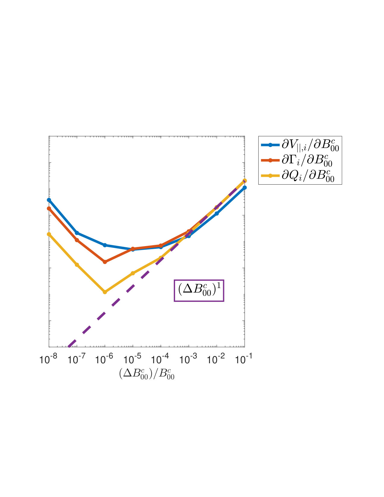 Figure 1
 Figure 2
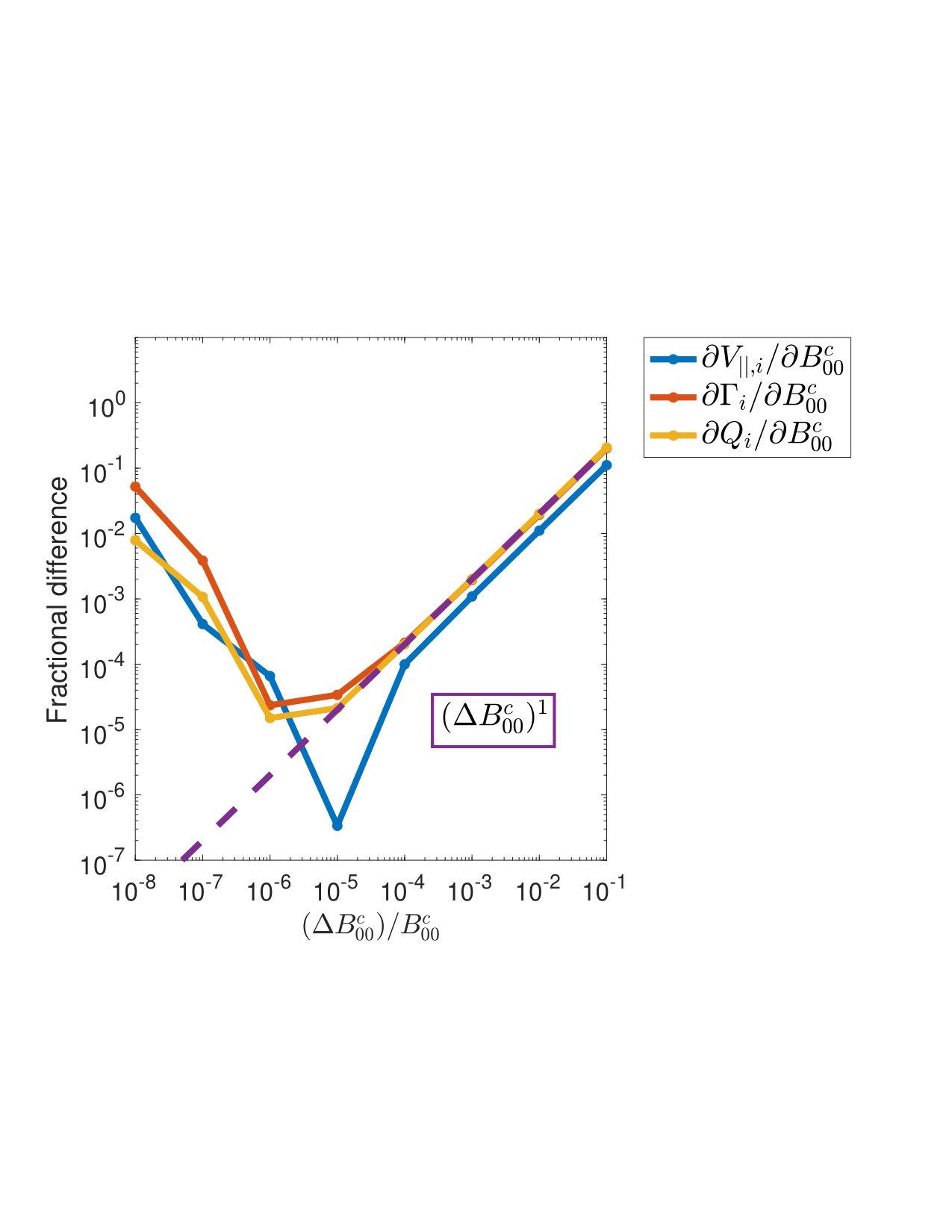 Figure 3
 Figure 4
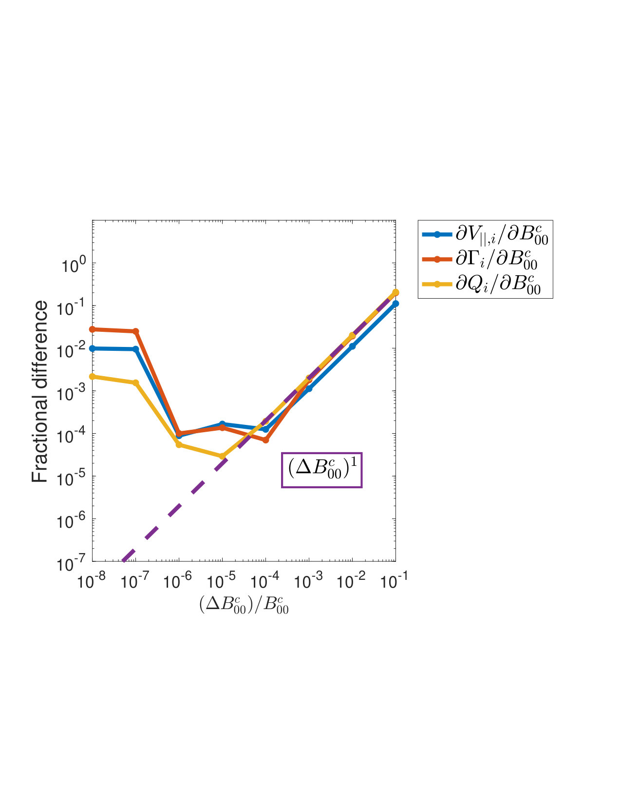 Figure 5
 Figure 6
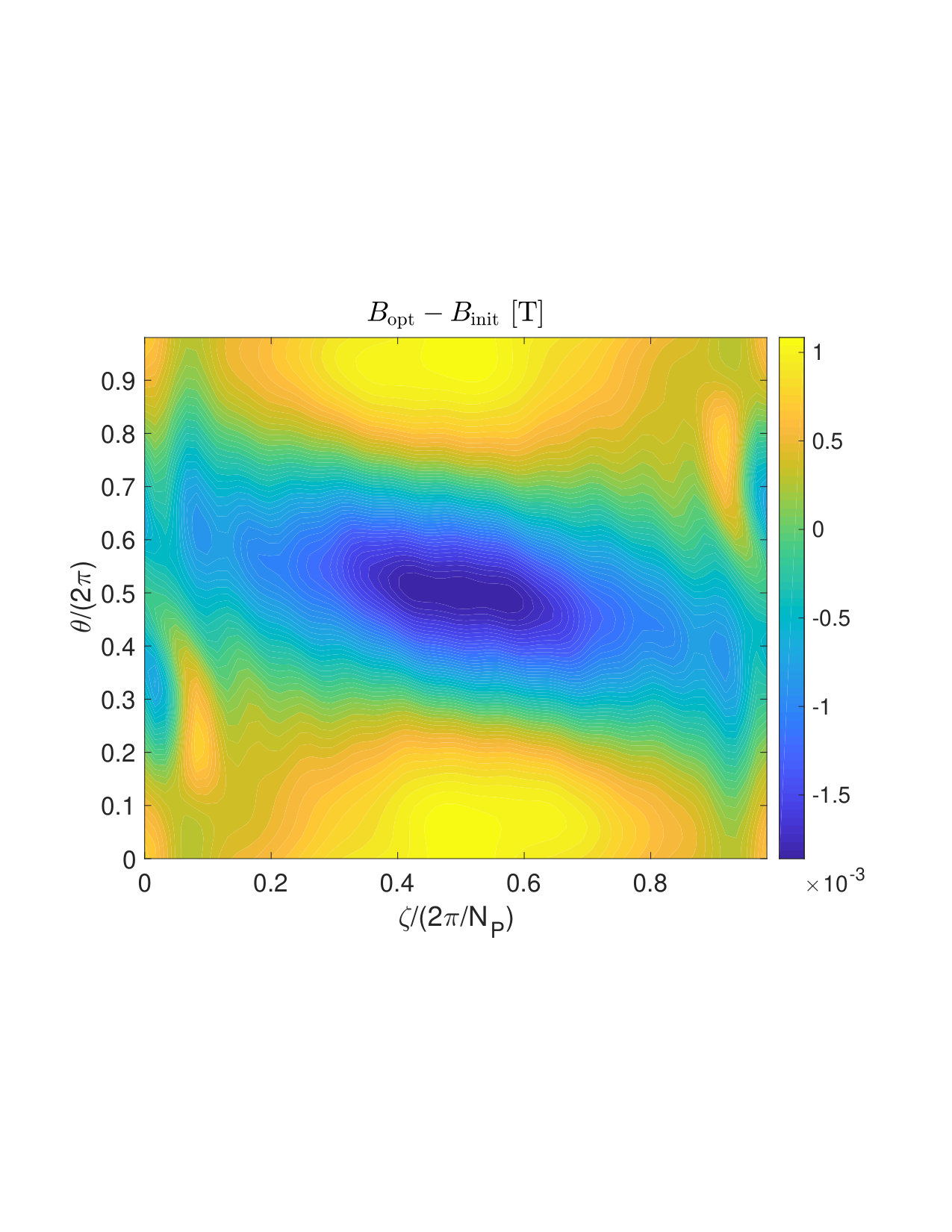 Figure 7
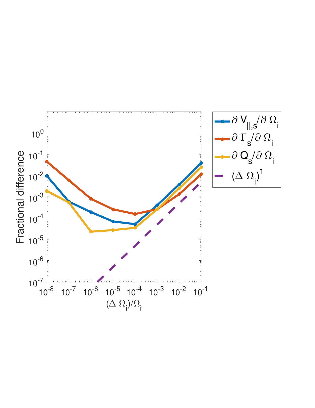 Figure 8
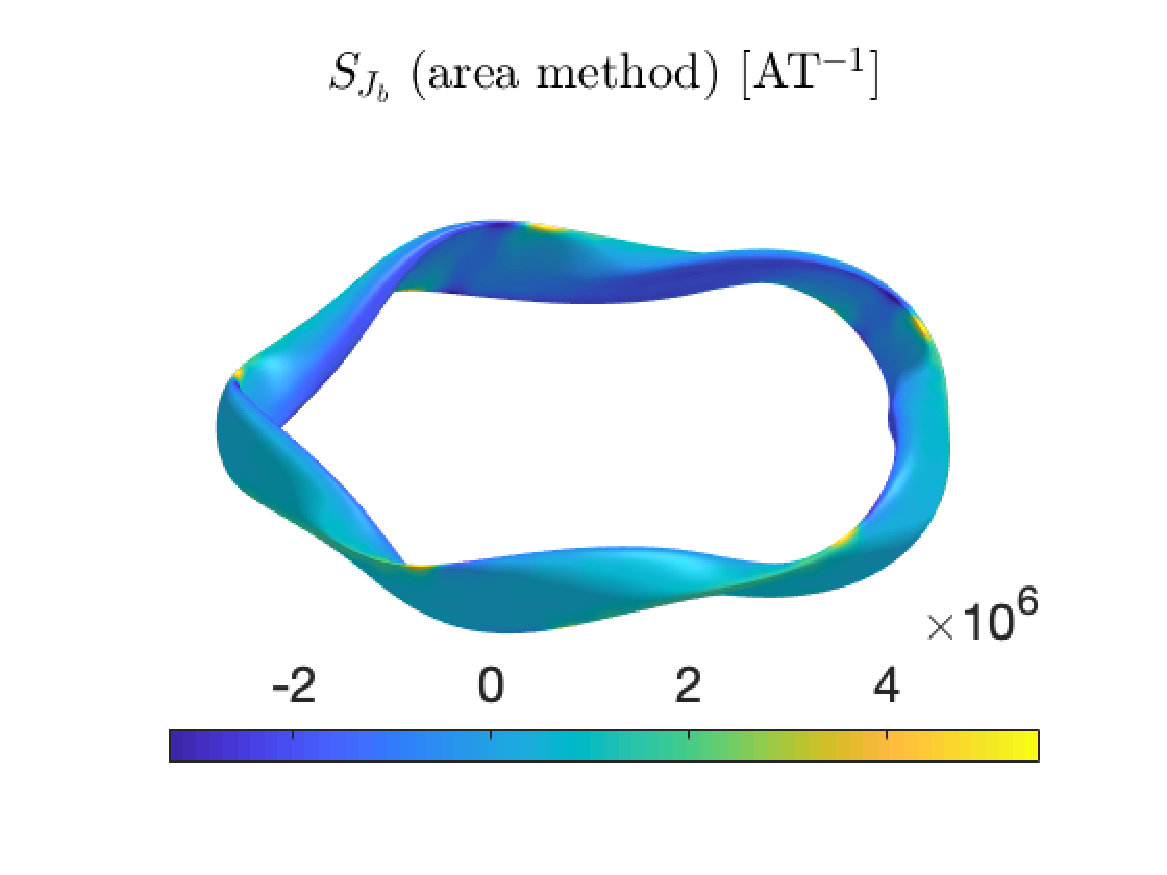 Figure 9
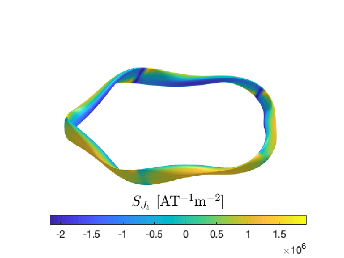 Figure 10
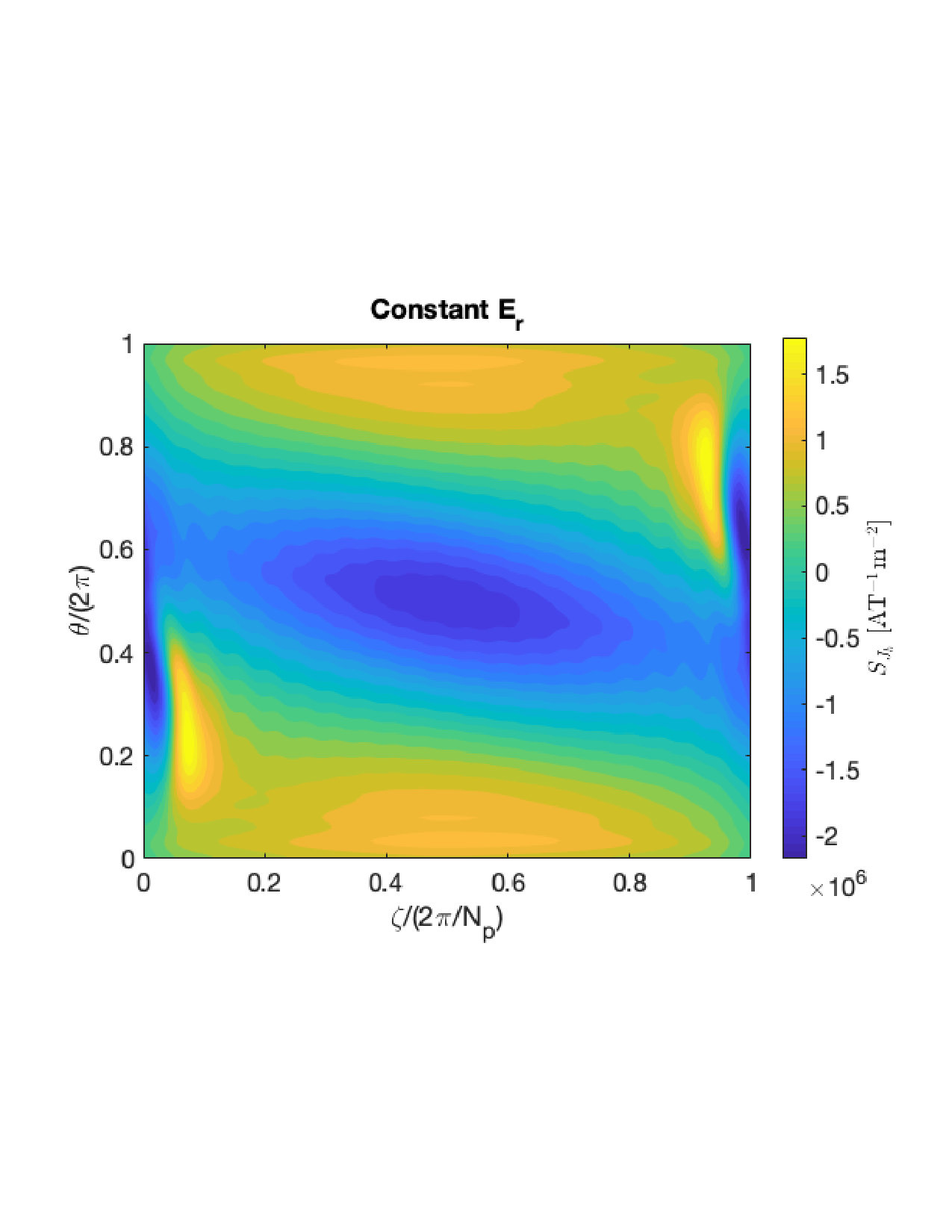 Figure 11
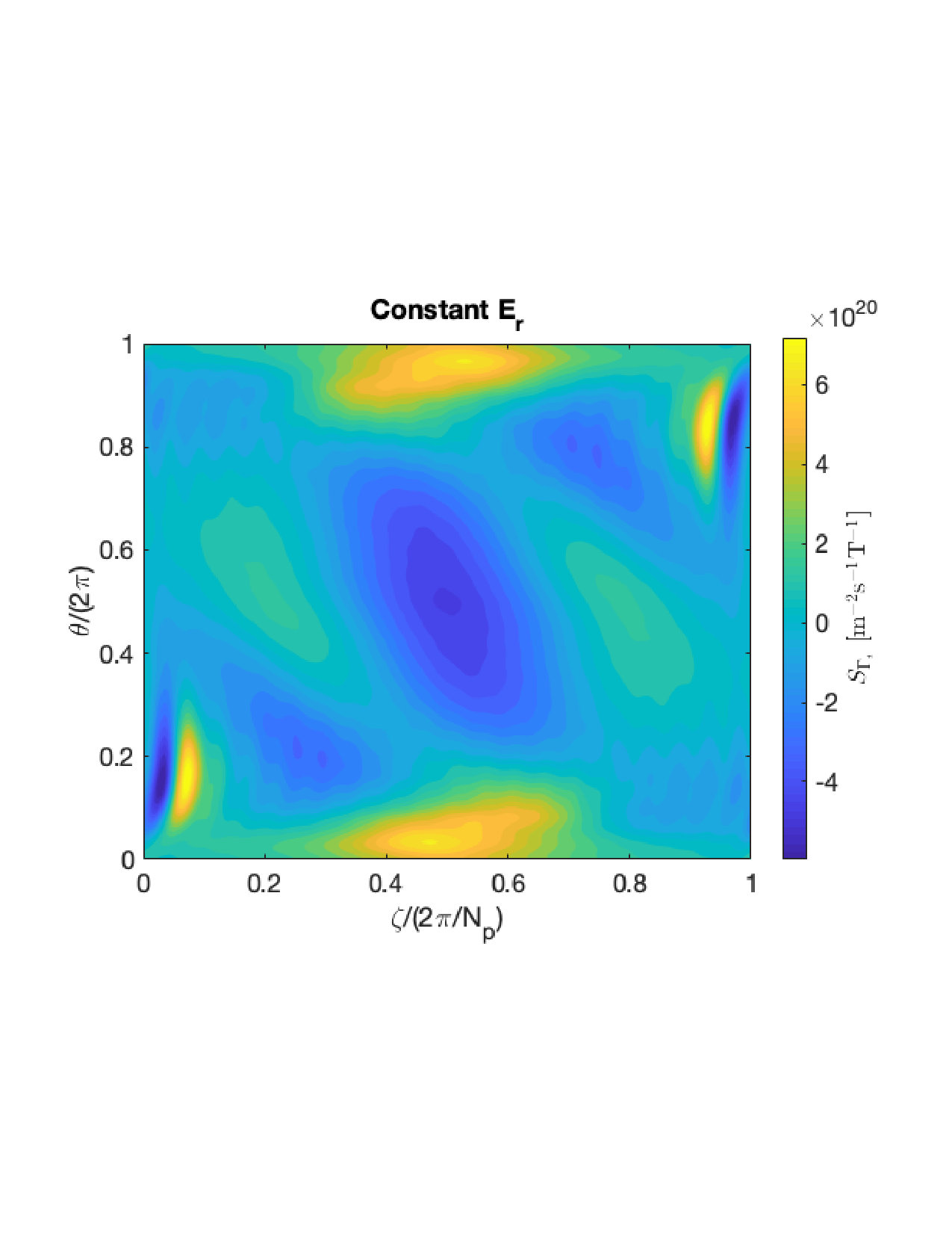 Figure 12
 Figure 13
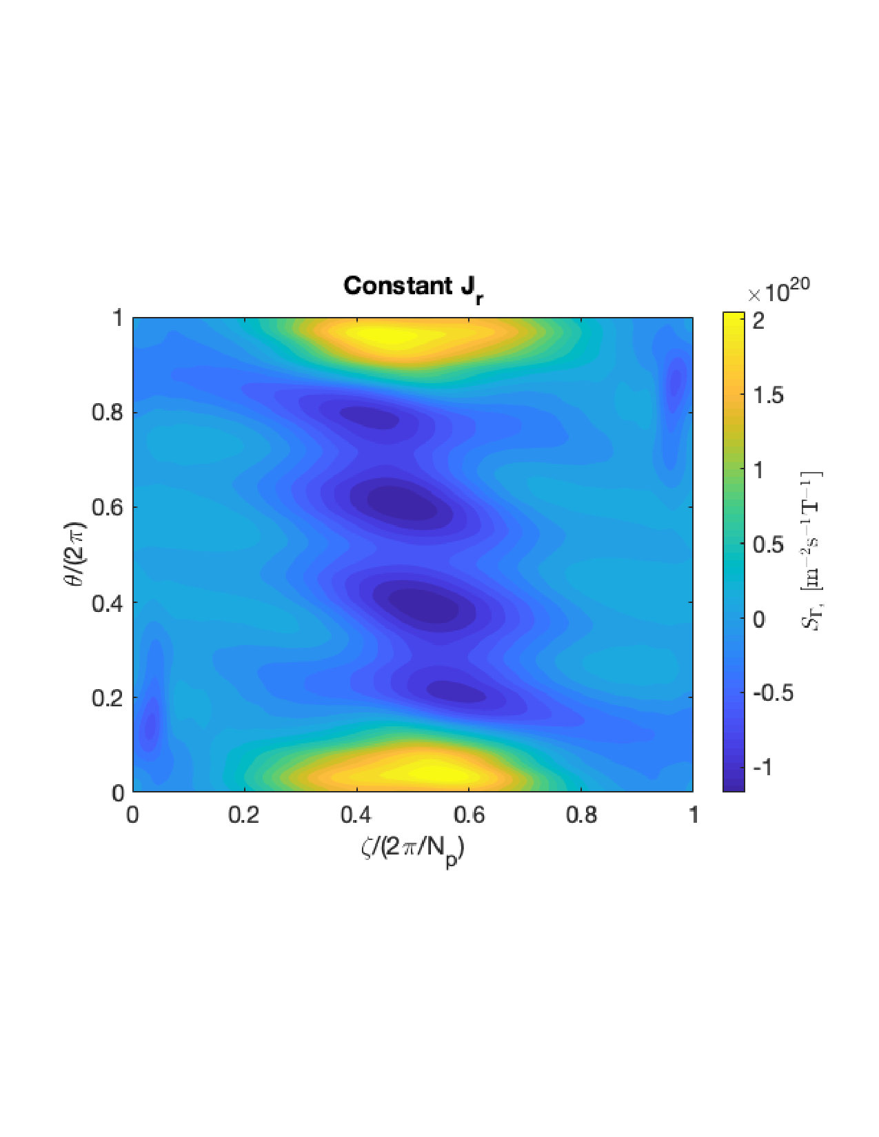 Figure 14
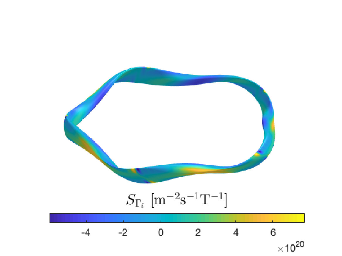 Figure 15
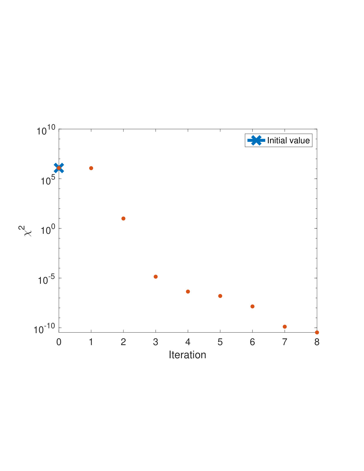 Figure 16
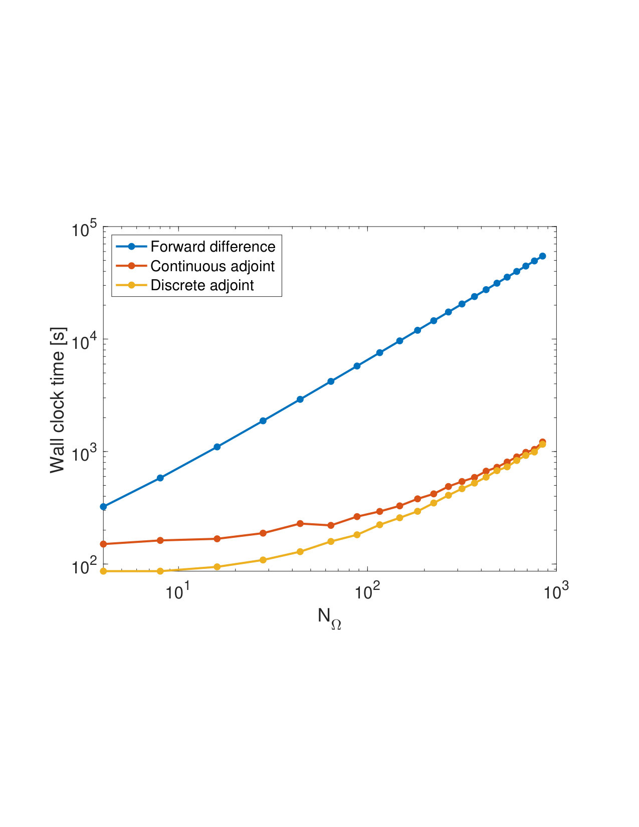 Figure 17
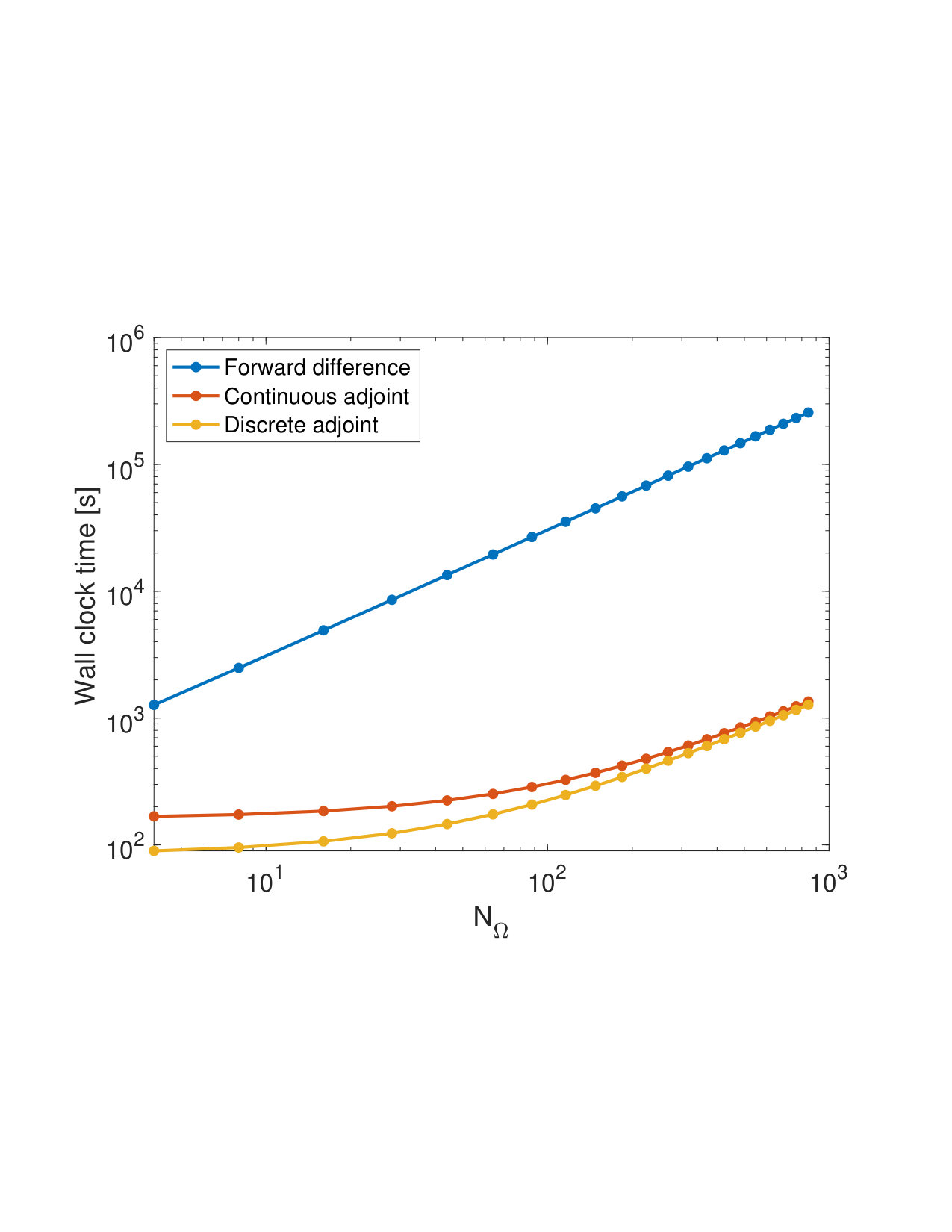 Figure 18
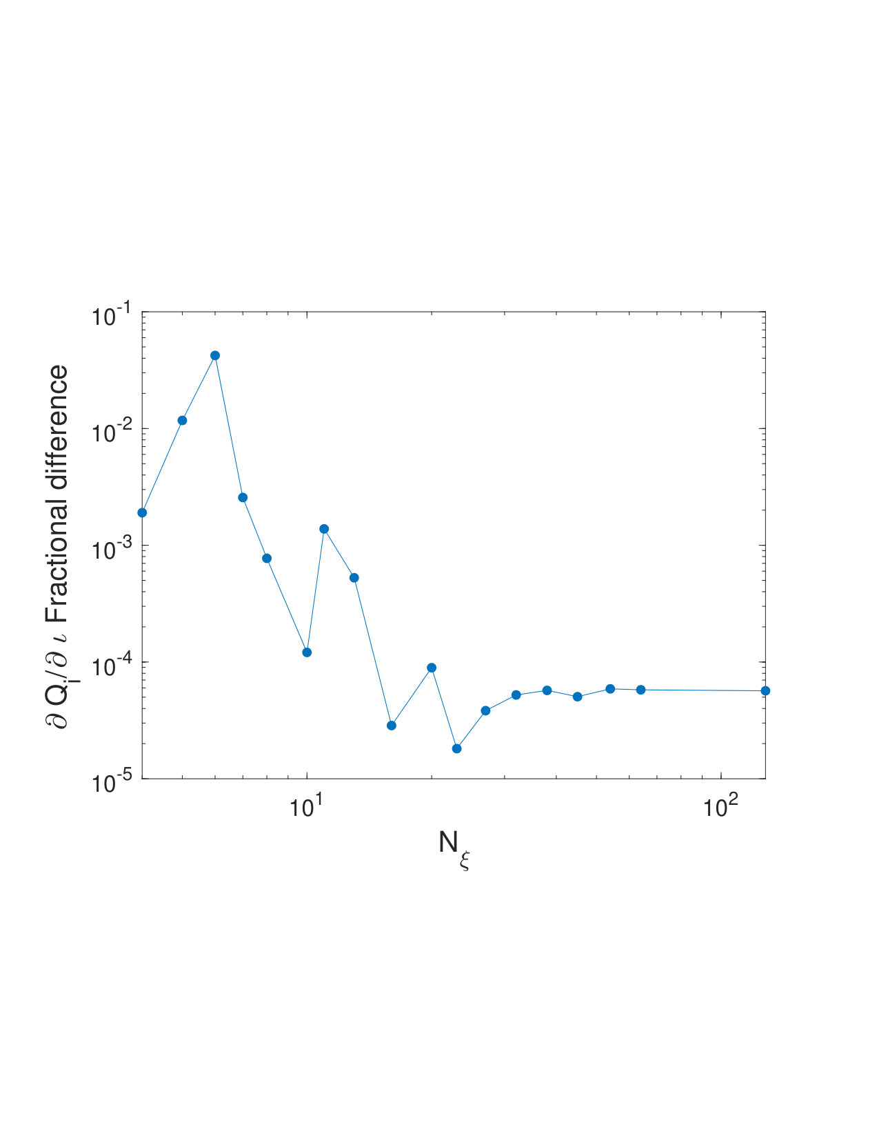 Figure 19
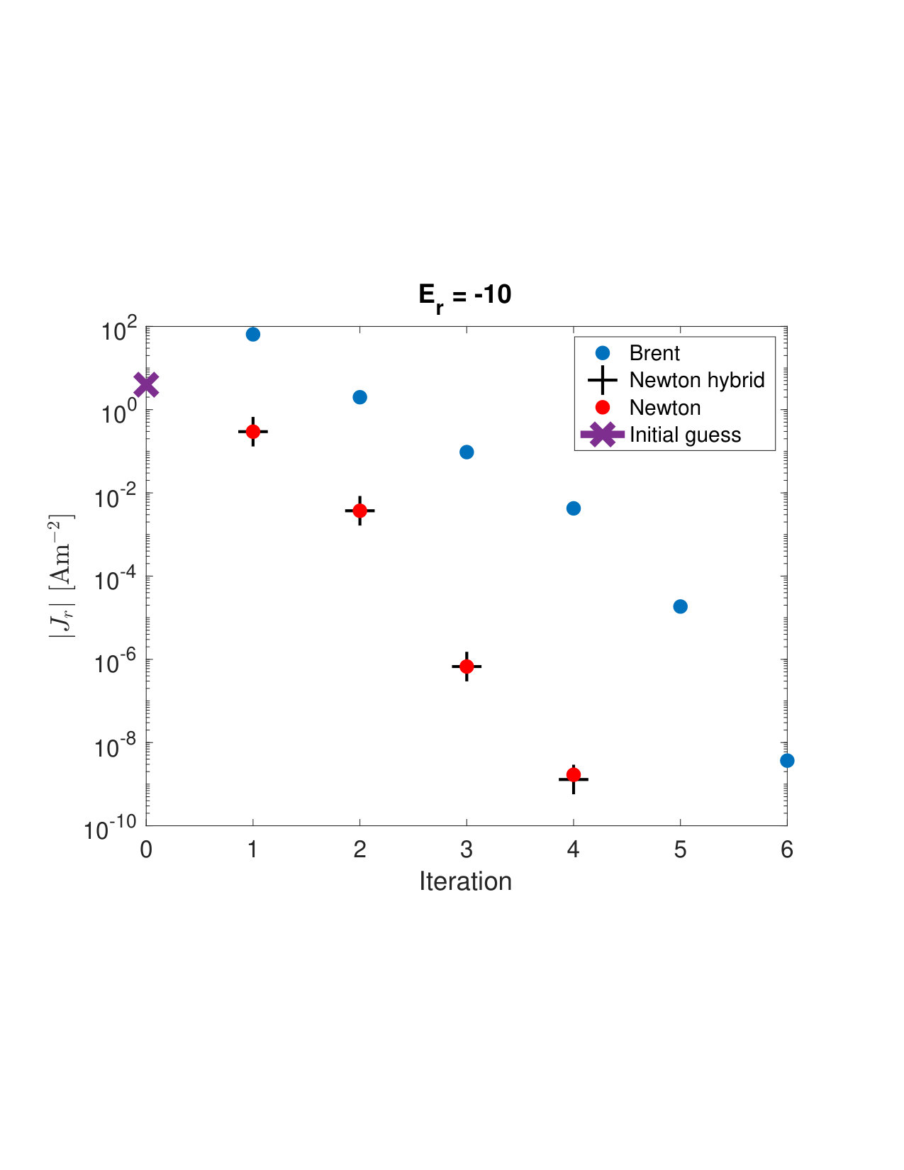 Figure 20
Peer Reviews
No public reviews on file for this paper yet. If you reviewed it on a platform where reviews are public (OpenReview, ICLR, NeurIPS, ICML), you can paste yours below so the community can read it here.
Videos
No videos yet. Explain this paper in a talk, walkthrough, or lecture? Add one.
An adjoint method for neoclassical stellarator optimization
Elizabeth J. Paul\aff1\[email protected]
Ian G. Abel\aff1,2
Matt Landreman\aff1
William Dorland\aff1
\aff1 Institute for Research in Electronics and Applied Physics, University of Maryland, College Park, MD 20742, USA \aff2Department of Physics, Chalmers University of Technology, Göteborg, SE-41296, Sweden
Abstract
Stellarators are a promising route to steady-state fusion power. However, to achieve the required confinement, the magnetic geometry must be highly optimized. This optimization requires navigating high-dimensional spaces, often necessitating the use of gradient-based methods. The gradient of the neoclassical fluxes is expensive to compute with classical methods, requiring flux computations, where is the number of parameters. To reduce the cost of the gradient computation, we present an adjoint method for computing the derivatives of moments of the neoclassical distribution function for stellarator optimization. The linear adjoint method allows derivatives of quantities which depend on solutions of a linear system, such as moments of the distribution function, to be computed with respect to many parameters from the solution of only two linear systems. This reduces the cost of computing the gradient to the point that the finite-collisionality neoclassical fluxes can be used within an optimization loop.
With the neoclassical adjoint method, we compute solutions of the drift kinetic equation and an adjoint drift kinetic equation to obtain derivatives of neoclassical quantities with respect to geometric parameters. When the number of parameters in the derivative is large (), this adjoint method provides up to a factor of 200 reduction in cost. We demonstrate adjoint-based optimization of the field strength to obtain minimal bootstrap current on a surface. With adjoint-based derivatives, we also compute the local sensitivity to magnetic perturbations on a flux surface and identify regions where tight tolerances on error fields are required for control of the bootstrap current or radial transport. Furthermore, the solve for the ambipolar electric field is accelerated using a Newton method with derivatives obtained from the adjoint method.
1 Introduction
The stellarator is a promising approach to magnetic confinement, as it does not require plasma current to produce rotational transform and thus is inherently steady-state and stable to current-driven modes. However, collisionless trajectories are not guaranteed to be confined in three-dimensional geometry as they are in axisymmetric systems (Gibson & Taylor, 1967; Helander, 2014). This can lead to poor confinement of energetic particles and increased neoclassical transport. A possible solution is the application of numerical optimization techniques to carefully tailor the magnetic geometry for improved confinement properties. One of the first demonstrations of this technique was in the design of the Wendelstein 7-X (W7-X) stellarator (Grieger et al., 1992; Lotz et al., 1990), which was optimized for small neoclassical transport in the regime and for small bootstrap current, in addition to several other physics criteria.
Another approach to improve confinement in stellarators is to obtain a configuration whose magnetic field strength exhibits a symmetry direction when expressed in Boozer coordinates, known as quasi-symmetry (Nührenberg & Zille, 1988). This leads to a conserved canonical momentum of the guiding center motion such that neoclassical properties are similar to those in a tokamak. However, perfect quasi-symmetry can never been achieved globally in practice (Garren & Boozer, 1991; Landreman & Sengupta, 2018), and it is often desirable to include symmetry-breaking components of the magnetic field strength in consideration of other design parameters, such as magneto-hydrodynamic (MHD) stability and energetic particle confinement (Nelson et al., 2003; Henneberg et al., 2019). As one must allow for breaking of quasi-symmetry, it remains essential to include a measure of neoclassical transport such that the symmetry-breaking harmonics of the field strength do not significantly degrade the confinement.
Neoclassical transport is governed by solutions of the drift kinetic equation, (DKE) (1), from which moments (e.g. radial fluxes and bootstrap current) are computed. The DKE local to a flux surface can be solved numerically (Landreman et al., 2014; Belli & Candy, 2015). However, this four-dimensional problem is expensive to solve within an optimization loop, especially in low-collisionality regimes for which increased pitch-angle resolution is required to resolve the collisional boundary layer.
Therefore, it may be desirable to consider an analytic reduction of the DKE. Under the assumption of low collisionality, a bounce-averaged DKE can be considered (Beidler & D’haeseleer, 1995; Calvo et al., 2018). While bounce-averaging can significantly reduce the computational cost by decreasing the spatial dimensionality, this approach typically requires restrictions on the geometry, such as closeness to omnigeneity or a model magnetic field. Additional reduction of the DKE can be made in low collisionality regimes, resulting in semi-analytic expressions. For example the effective ripple, (Nemov et al., 1999), quantifies the geometric dependence of the radial transport and has been widely used during optimization studies (Zarnstorff et al., 2001; Ku et al., 2008; Henneberg et al., 2019). This model, though, assumes very small , which is not always an experimentally-relevant regime. A low-collisionality semi-analytic bootstrap current model (Shaing et al., 1989) is also commonly adopted for stellarator design (Beidler et al., 1990; Hirshman et al., 1999). However, this analytic expression is known to to be ill-behaved near rational surfaces. Furthermore, benchmarks with numerical solutions of the DKE in the low-collisionality limit have been shown to differ significantly from the semi-analytic model (Beidler et al., 2011; Kernbichler et al., 2016). Any analytic reduction of the DKE implies additional assumptions, such as on the collisionality, size of , or on the magnetic geometry.
Due to the limitations of bounce-averaged and semi-analytic models, there are benefits to computing neoclassical quantities using numerical solutions to the DKE without approximation. With the numerical methods currently used for stellarator optimization, this approach becomes computationally challenging within an optimization loop. Due to their fully three-dimensional nature, optimization of stellarator geometry requires navigation through high-dimensional spaces, such as the space of the shape of the outer boundary of the plasma or the shapes of electromagnetic coils. The number of parameters required to describe these spaces, , is often quite large (). Knowledge of the gradient of the objective function with respect to these parameters can greatly improve the convergence to a local minimum. Once a descent direction is identified, each iteration reduces to a one-dimensional line search. Gradient-based optimization with the Levenberg-Marquardt algorithm in the STELLOPT code (Strickler et al., 2004) has been widely-used in the stellarator community and led to the design of NCSX (Reiman et al., 1999).
Although derivative information is valuable, numerically computing the derivative of a figure of merit (for example, with finite difference derivatives) can be prohibitively expensive, as must be evaluated times. For neoclassical optimization, this implies solving the DKE times; thus including finite-collisionality neoclassical quantities in the objective function is often impractical. In this work we describe an adjoint method for neoclassical optimization. With this method, the computation of the derivatives of with respect to parameters has cost comparable to solving the DKE twice, thus making the inclusion of these quantities possible within an optimization loop. In this work we obtain derivatives of neoclassical figures of merit with respect to local geometric parameters on a surface rather than the outer boundary or coil shapes. However, the geometric derivatives we compute provide an important step toward adjoint-based optimization of MHD equilibria, as discussed in section 5.2.2.
Adjoint methods have been applied in many fields including aerodynamic engineering and computational fluid dynamics (Pironneau, 1974; Glowinski & Pironneau, 1975), geophysics (Plessix, 2006; Fichtner et al., 2006), structural engineering (Allaire et al., 2005), and tokamak divertor design (Dekeyser et al., 2014a, b, c). They have only recently been implemented for stellarator design, namely for the design of coil shapes (Paul et al., 2018) and efficiently computing shape gradients for MHD equilibria (Antonsen et al., 2019). The numerical method is quite general and has the potential to greatly impact many inverse design problems in magnetic confinement fusion.
In section 2 we provide an overview of the numerical solution of the DKE local to a flux surface. In section 3 the adjoint neoclassical method is described. Two approaches to the adjoint method, termed continuous and discrete, are presented, and their implementation and benchmarks are discussed in section 4. The adjoint method is used to compute derivatives of moments of the neoclassical distribution function with respect to local geometric quantities. The derivative information can be used to identify regions of increased sensitivity to magnetic perturbations, as discussed in section 5.1. We demonstrate adjoint-based optimization in section 5.2.1 by locally modifying the field strength on a flux surface. A discussion of the application of this method for optimization of MHD equilibria is presented in 5.2.2. Finally, the adjoint method is applied to accelerate the calculation of the ambipolar electric field in section 5.3.
2 Drift kinetic equation
The Stellarator Fokker-Planck Iterative Neoclassical Solver (SFINCS) code (Landreman et al., 2014) solves the drift kinetic equation,
[TABLE]
for general stellarator geometry. Here is a unit vector in the direction of the magnetic field, is the parallel component of the velocity, and is the toroidal flux. The Fokker-Planck collision operator is , linearized about a Maxwellian where is the thermal speed, is the density, is the temperature, is the mass, and the subscript indicates species. In (1), derivatives are performed holding and fixed, where is the magnitude of velocity, is the electrostatic potential, is the perpendicular velocity, and is the charge. The radial magnetic drift is
[TABLE]
assuming a magnetic field in MHD force balance, and is the velocity
[TABLE]
Throughout we assume such that (1) is linear. In (1) we will not consider the effect of inductive electric fields, as this can be assumed to be small for stellarators without inductive current drive. We also do not consider the effects of magnetic drifts tangential to the flux surface in (1), as these only become important when is small (Paul et al., 2017).
SFINCS solves (1) locally on a flux surface , thus it is four-dimensional. The SFINCS coordinates include two angles (poloidal angle and toroidal angle ), speed , and pitch angle . Specifics about the implementation of (1) in the SFINCS code are described in appendix A. We will refer to two choices of implementation, the full trajectory model and the DKES trajectory model. The full trajectory model maintains conservation as radial coupling (terms involving ) is dropped. While the DKES model does not conserve when the radial electric field , the adjoint operator under the DKES model takes a particularly simple form as discussed in section 3.1. This model also does not introduce any unphysical constraints on the distribution function when , as occurs for the full trajectory model (Landreman et al., 2014). These constraints motivate the introduction of particle and heat sources, which are discussed in the following section. We will discuss some of the details of the implementation of the DKE in the SFINCS code as these need to be considered in arriving at the adjoint equation. However, the adjoint neoclassical approach is quite general and could be implemented in other drift kinetic codes with slight modification.
From solutions of (1), several neoclassical quantities are computed, including the flux surface averaged parallel flow,
[TABLE]
the radial particle flux,
[TABLE]
and the radial heat flux (sometimes referred to as an energy flux),
[TABLE]
We will also consider species-summed quantities including the bootstrap current, , the radial current, , and the total heat flux, . Here the effective normalized radius is , where is the toroidal flux at the boundary.
2.1 Sources and constraints
To avoid unphysical constraints on implied by the moment equations of (1) in the presence of a non-zero (Landreman et al., 2014), particle and heat sources are added to the DKE (73),
[TABLE]
where and are unknowns such that provides a particle source and provides a heat source. The collisionless trajectory operator in SFINCS coordinates is
[TABLE]
and the inhomogeneous drive term is . The source functions are determined via the requirement that and (i.e. does not provide net density or pressure). So, the following system of equations is solved,
[TABLE]
The velocity-space averaging operations are denoted and . The full multi-species system can be written as,
[TABLE]
Here the linear systems corresponding to each species as in (18) are coupled through the collision operator. We use the following notation to refer to the above system,
[TABLE]
3 Adjoint approach
The goal of the adjoint neoclassical approach is to efficiently compute derivatives of a moment of the distribution function, (e.g. , with respect to many parameters. Consider a set of parameters, , on which depends. Computing a forward difference derivative with respect to requires solutions of (29). With the adjoint approach, can be computed with one solution of (29) and one solution of a linear adjoint equation of the same size as (29). Thus if is very large and the solution to (29) is computationally expensive to obtain, the adjoint approach can reduce the cost by . For stellarator optimization, it is desirable to compute derivatives with respect to parameters which describe the magnetic geometry. In fully three-dimensional geometry, is and solving (29) is the most expensive part of computing (rather than constructing the linear system or taking a moment of the distribution function). Thus the adjoint approach can provide a computational savings of a factor of . The adjoint method is also advantageous over numerical derivatives, as it avoids additional noise from discretization error. In what follows we consider to be a set of parameters describing the magnetic geometry, which will be specified in section 4.
We compute the derivatives of using two approaches. In the first approach, we define an inner product which involves integrals over the distribution function, and an adjoint operator is obtained with respect to this inner product. This we refer to as the continuous approach. In the second approach, we consider the DKE after discretization, defining an adjoint operator with respect to the Euclidean dot product. This we refer to as the discrete approach. While these approaches should provide identical results within discretization error, the advantages and drawbacks of each approach will be discussed at the end of section 3.2.
3.1 Continuous approach
Let be the set of unknowns computed with SFINCS before discretization, denoted by the column vector in (28) with given by (18). That is, consists of a set of distribution functions over and their associated source functions. We define an inner product between two such quantities in the following way,
[TABLE]
Here the superscript on and denotes the distribution function with which the source functions are associated and the sum is over species. The space of continuous functions, , of this form such that is bounded will be denoted by . It can be seen that (30) is indeed an inner product, as it satisfies conjugate symmetry ( ), linearity ( and , ), and positive definiteness ( and only if ) (Rudin, 2006). This implies that if is finite-dimensional, then for any linear operator there exists a unique adjoint operator such that for all . While here is not finite-dimensional, we will show that such an adjoint operator exists for this inner product.
Note that the norm associated with this inner product is similar to the free energy norm,
[TABLE]
which obeys a conservation equation in gyrokinetic theory (Krommes & Hu, 1994; Abel et al., 2013; Landreman et al., 2015). The choice of inner product (30) is advantageous, as the linearized Fokker-Planck collision operator becomes self-adjoint for species linearized about Maxwellians with the same temperature. In what follows, we assume that all included species are of the same temperature. This assumption could be lifted, with a modification to the collision operator that appears in the adjoint equation (see appendix B). This assumption is not necessary when using the discrete approach (see section 3.2).
Consider a moment of the distribution function , which can be written as an inner product with a vector ,
[TABLE]
according to (30). For example,
[TABLE]
where the column structure corresponds with that in (18) and (28).
We are interested in computing the derivative of with respect to a set of parameters, . This derivative can be computed with the chain rule,
[TABLE]
The subscripts in (37) denote the quantity that is held fixed while the derivative is computed. The first term on the right hand side accounts for the explicit dependence on while the second accounts for the implicit dependence on through . Here can be computed by considering perturbations to the linear system (29), noting that in general both and can depend on ,
[TABLE]
Computing using (38) requires solving linear systems of the same dimension as the DKE (29). To avoid this additional computational cost, we instead solve an adjoint equation,
[TABLE]
In what follows, we show that the adjoint variable, , can be used to compute without solving (38) for each . Using (39) with (37),
[TABLE]
and applying the adjoint property, we obtain
[TABLE]
Using (38),
[TABLE]
So, (42) provides the same derivative information as (37). Thus, using (42), the derivative with respect to can be computed with the solution to two linear systems, (29) and (39). The partial derivatives on the right hand side of (42) can be computed analytically by considering the explicit geometric dependence of , , and .
When is large, the cost of computing using (42) is dominated not by the linear solve but by constructing and and computing the inner product. Thus the cost still scales with . However, we obtain a significant savings in comparison with forward difference derivatives, as shown in section 4.
The adjoint operator for each species takes the following form,
[TABLE]
where and . The same column structure is used as for the forward operator (28), . The quantity satisfies and depends on which trajectory model is applied. The expression (46) can be verified by noting that
[TABLE]
For the DKES trajectories the adjoint operator is,
[TABLE]
This anti-self-adjoint property is used in obtaining the variational principle which provides bounds on neoclassical transport coefficients in the DKES code (van Rij & Hirshman, 1989). For full trajectories it is,
[TABLE]
The anti-self-adjoint property does not hold for this trajectory model as the drift (91) is no longer divergenceless. See appendix C for details on obtaining these adjoint operators.
3.2 Discrete approach
Next we consider the discrete adjoint approach. Let be the set of unknowns computed with SFINCS after discretization of . The linear DKE (29) upon discretization can then be written schematically as
[TABLE]
In this case, we can define an inner product as the vector dot product,
[TABLE]
In real Euclidean space, the adjoint operator, , which satisfies
[TABLE]
is simply the transpose of the matrix, . Again, the moments of the distribution function, can be expressed as an inner product with a vector ,
[TABLE]
Using the discrete approach, the following adjoint equation must be solved
[TABLE]
The adjoint variable, , can again be used to compute ,
[TABLE]
As with the continuous approach, the partial derivatives on the right hand side can be computed analytically. In this way, the derivative of with respect to can be computed with only two linear solves, (50) and (54).
In the SFINCS implementation, the DKE is typically solved with the preconditioned GMRES algorithm. In the continuous approach, a preconditioner matrix for both the forward and adjoint operator must be -factorized. Here the preconditioner matrix is the same as the full matrix but without cross-species or speed coupling. As the adjoint matrix is sufficiently different from the forward matrix, we do not obtain convergence when the same preconditioner is used for both problems. However, in the discrete approach, the -factorization for the preconditioner of the forward matrix can be reused for the preconditioner of the adjoint matrix (If a matrix has been factorized as then where is lower triangular and is upper triangular). This provides a significant reduction in memory and computational cost for the discrete approach.
Furthermore, the discrete adjoint approach provides the exact derivatives for the discretized problem. With this method the adjoint equation is obtained using the vector dot product and matrix transpose which can be computed without any numerical approximation. The error in the derivatives obtained by the adjoint method are therefore only limited by the tolerance to which the linear solve is performed with GMRES. On the other hand, the continuous adjoint approach relies on a continuous inner product which must ultimately be approximated numerically. Thus the continuous approach provides the exact derivatives only in the limit that the discrete approximation of the inner product exactly reproduces the continuous inner product. Therefore we expect the results of the discrete and adjoint approaches to agree within discretization error, as will be demonstrated in section 4.
The continuous approach can be advantageous in that an adjoint equation may be prescribed independently of the discretization scheme. Note that in the discrete approach, the adjoint operator is obtained from the matrix transpose of the discretized forward operator, which implies that the same spatial and velocity resolution parameters must be used for both the forward and adjoint solutions. In this work we will employ the same discretization parameters for both the adjoint and forward problems, but this restriction is not required for the continuous approach.
4 Implementation and benchmarks
The adjoint method has been implemented in the SFINCS code using both the discrete and continuous approaches. The magnetic geometry is specified in Boozer coordinates (Helander, 2014) such that the covariant form of the magnetic field is,
[TABLE]
where and , is the toroidal current enclosed by , and is the poloidal current outside of . The contravariant form is
[TABLE]
where is the rotational transform. The Jacobian is obtained from dotting (56) with (57),
[TABLE]
As does not appear in any of the trajectory coefficients ((74) and (77)), in the drive term in (73), or in the geometric factors used to define the moments of the distribution function (4, 5 and 6), all the geometric dependence enters through , , , and . We choose to use Boozer coordinates for these computations as it reduces the number of geometric parameters that must be considered, but the neoclassical adjoint method is not limited to this choice of coordinate system.
We approximate by a truncated Fourier series,
[TABLE]
where sums over Fourier modes and such that is an integer multiple of , the number of field periods. In (59), we have assumed stellarator symmetry such that , and symmetry such that . Thus we compute derivatives with respect to the parameters }. Additionally, derivatives with respect to are computed, which are used for efficient ambipolar solutions and computing derivatives of geometric quantities at ambipolarity (see section 5.3) rather than at fixed .
To demonstrate, we compute for moments of the ion distribution function using the discrete and continuous adjoint methods. A 3-mode model of the standard configuration W7-X geometry at is used (table 1 in Beidler et al. (2011)),
[TABLE]
where , , and . Electron and ion () species are included, and the derivatives are computed at the ambipolar with the full trajectory model. The derivatives are also computed with a forward difference approach with varying step size . In figure 1 we show the fractional difference between computed using the adjoint method and with forward difference derivatives. We see that at large values of , the adjoint and numerical derivatives begin to differ significantly due to discretization error from the forward difference approximation. The fractional error decreases proportional to as expected until the rounding error begins to dominate (Sauer, 2012) when is approximately , where is the value of the unperturbed mode. The discrete and continuous approaches show qualitatively similar trends, though the minimum fractional difference is lower in the discrete approach due to the additional discretization error that arises with the continuous approach. With sufficient resolution parameters (41 grid points, 61 grid points, 85 basis functions, and 7 basis functions), the fractional error of the continuous approach is and should not be significant for most applications. We find similar agreement for other derivatives and with the DKES trajectory model.
To demonstrate that the discrete and continuous methods indeed produce the same derivative information, we compute the fractional difference between the derivatives computed with the two methods as a function of the resolution parameters. As an example, in figure 2(a) we show the fractional difference in , where is the radial ion heat flux, as a function of the number of Legendre polynomials used for the pitch angle discretization, , keeping the other resolution parameters fixed. As is increased, the fractional differences converges to a finite value, approximately , due to the discretization error in the other resolution parameters. Similar resolution parameters are required for the convergence of the moment itself, , and its derivative computed with the continuous method, . Convergence of within 5% is obtained with , similar to that required for the convergence of , as can be seen in figure 2(a).
In figure 2(b) we compare the cost of calculating derivatives of one moment with respect to parameters using the continuous and discrete adjoint methods and forward difference derivatives. All computations are performed on the Edison computer at NERSC using 48 processors, and the elapsed wall time is reported. Here we include the cost of solving the linear system and computing diagnostics times for the forward difference approach, and the cost of solving the forward and adjoint linear systems and computing diagnostics for the adjoint approaches. The cost of the continuous approach is slightly more than that of the discrete approach due to the cost of factorizing the adjoint preconditioner. However, at large the cost of computing diagnostics for the adjoint approach (e.g. computing and and performing the inner product in (42)) dominates that of solving the adjoint linear system; thus the discrete and continuous approaches become comparable in cost. In this regime, the adjoint approach provides speed-up by a factor of approximately .
5 Applications of the adjoint method
5.1 Local magnetic sensitivity analysis
Using the adjoint method, it is possible to compute derivatives of a moment of the distribution function with respect to the Fourier amplitudes of the field strength, . Rather than consider sensitivity in Fourier space, we would like to compute the sensitivity to local perturbations of the field strength. We now quantify the relationship between these two representations of sensitivity information.
Consider the Gâteaux functional derivative (Delfour & Zolâsio, 2011) of with respect to ,
[TABLE]
Here we consider a perturbation to the field strength at fixed , , and . As is a linear functional of , by the Riesz representation theorem (Rudin, 2006), can be expressed as an inner product with and some element of the appropriate space. The function is defined on a flux surface, ; thus it is sensible to express in the following way,
[TABLE]
Here describes the local perturbation to the field strength, and quantifies the corresponding change to the moment . The function is analogous to the shape gradient, which quantifies the change in a figure of merit which results from a differential perturbation to a shape (Landreman & Paul, 2018). The shape gradient will be discussed further in section 5.2.2.
Suppose that is stellarator symmetric and symmetric. If , then must also possess stellarator and symmetry (see appendix D). However, when , is no longer guaranteed to have stellarator symmetry. Nonetheless, it may be desirable to ignore the stellarator-asymmetric part of if an optimized stellarator-symmetric configuration is desired. For the remainder of this work, we will make this assumption, though the analysis could be extended to consider the effect of breaking of stellarator symmetry. The quantity can be approximated by a truncated Fourier series under these assumptions,
[TABLE]
where sums over and such that is an integer multiple of . The quantity can be written in terms of perturbations to the Fourier coefficients,
[TABLE]
where again the sum is only taken over symmetric modes. Now can be written in terms of perturbations to the Fourier coefficients,
[TABLE]
In this way, (62) can be expressed as a linear system,
[TABLE]
where
[TABLE]
If the same number of modes is used to discretize and , then the linear system is square.
In contrast to derivatives with respect to the Fourier modes of , the sensitivity function, , is a spatially local quantity, quantifying the change in a figure of merit resulting from a local perturbation of the field strength. In this way, can inform where perturbations to the magnetic field strength can be tolerated. The sensitivity function could be related directly to a local magnetic tolerance using the method described in section 9 of (Landreman & Paul, 2018). In contrast with that work, here we are considering perturbations to the field strength on any flux surface rather than at the plasma boundary. However, still provides insight into where trim coils should be placed or coil displacements can be tolerated without sacrificing desired neoclassical properties. The sensitivity function can also be used for gradient-based optimization in the space of the field strength on a flux surface as in section 5.2.1.
We compute for the W7-X standard configuration at , shown in figure 3(a). We use a fixed-boundary equilibrium that preceded the coil design and does not include coil ripple, and the full equilibrium is used rather than the truncated Fourier series considered in section 4. The same resolution parameters are used as in section 4, and derivatives with respect to are computed for . The largest modes for this configuration are the helical curvature , the toroidal curvature , and the toroidal mirror . We find that is large and negative on the inboard side, indicating that increasing the magnitude of the toroidal curvature component of would lead to an increase in . This result is in agreement with previous analysis of the dependence of the bootstrap current on these three modes in the W7-X magnetic configuration space (Maassberg et al. (1993)), which found that at low collisionality the bootstrap current coefficients depend strongly on the toroidal curvature. In figure 3(b) is the sensitivity function for the ion particle flux, , computed for the same configuration using and . We find that the particle flux is more sensitive to perturbations on the outboard side in localized regions, while on the inboard side the sensitivity is relatively small in magnitude.
5.2 Gradient-based optimization
5.2.1 Optimization of field strength
As a second demonstration of the adjoint neoclassical method, we consider optimizing in the space of the field strength on a surface, taking . As Boozer coordinates are used, the covariant form (56) satisfies and the contravariant form (57) satisfies . As we will artificially modify the field strength while keeping other geometry parameters fixed, the resulting field will not necessarily satisfy both of these conditions with both the covariant and contravariant forms. While there is no guarantee that the resulting field strength will be consistent with a global equilibrium solution, it provides insight into how local changes to the field strength can impact neoclassical properties. As a second step, the outer boundary could be optimized to match the desired field strength on a single surface. In section 5.2.2, we discuss how the derivatives computed in this work could be coupled to optimization of an MHD equilibrium.
We perform optimization with a BFGS quasi-Newton method (Nocedal & Wright, 1999) using an objective function . A backtracking line search is used at each iteration to find a step size that satisfies a condition of sufficient decrease of . We use the same equilibrium as in section 5.1, retaining modes and , and compute derivatives with respect to these modes. Convergence to was obtained within 8 BFGS iterations (28 function evaluations), as shown in figure 4(a). The difference in field strength between the initial and optimized configuration, , is shown in figure 4(b). As expected from the analysis in section 5.1, the field strength increased on the outboard side and decreased on the inboard side in comparison with .
5.2.2 Optimization of MHD equilibria
The local sensitivity function, , along with , , and , can be used to determine how perturbations to the outer boundary of the plasma, , result in perturbations to . This is quantified through the idea of the shape gradient, which is described below. The partial derivatives of can be computed with the adjoint method outlined in section 3, and the shape gradient can be obtained with only one additional MHD equilibrium solution through the application of another adjoint method.
Consider a figure of merit which is integrated over a toroidal domain, ,
[TABLE]
where is a weighting function. That is, SFINCS is run on a set of surfaces within and the volume integral is computed numerically. Here we consider to be the plasma boundary used for a fixed-boundary MHD equilibrium calculation. The perturbation to resulting from normal perturbation to can be written in the following form,
[TABLE]
under certain assumptions of smoothness (Delfour & Zolésio, 2011). This can be thought of as another instance of the Riesz representation theorem, as is a linear functional of . Here is the outward unit normal on and is a vector field describing the perturbation to the surface. Intuitively, only normal perturbations to result in a change to . The shape gradient is , which quantifies the contribution of a local normal perturbation of the boundary to the change in . The shape gradient can be used for fixed-boundary optimization of equilibria or for analysis of sensitivity to perturbations of magnetic surfaces. It can be computed using a second adjoint method, where a perturbed MHD force balance equation is solved with the addition of a bulk force which depends on derivatives computed from the neoclassical adjoint method (Antonsen et al., 2019). While the continuous neoclassical adjoint method described in this work arises from the self-adjointness of the linearized Fokker-Planck operator, the adjoint method for MHD equilibria arises from the self-adjointness of the MHD force operator. In practice these two adjoint methods could be coupled by first computing an MHD equilibrium solution, computing neoclassical transport and its geometric derivatives from this equilibrium with the neoclassical adjoint method, and passing these derivatives back to the equilibrium code to compute the shape gradient with the perturbed MHD adjoint method. In this way derivatives of neoclassical quantities with respect to the shape of the outer boundary are computed with only two equilibrium solutions and two DKE solutions. This calculation will be reported in a future publication.
Rather than solve an additional adjoint equation, the outer boundary could be optimized by numerically computing derivatives of with respect to the double Fourier series describing the outer boundary shape in cylindrical coordinates, , using a finite difference method. This could be done using the STELLOPT code (Spong et al., 1998; Reiman et al., 1999) with BOOZ_XFORM (Sanchez et al., 2000) to perform the coordinate transformation. For example, if the rotational transform is held fixed in the VMEC equilibrium calculation (Hirshman & Whitson, 1983), the derivative of a moment, , with respect to a boundary coefficient, , can be computed as,
[TABLE]
where , , and are computed with the neoclassical adjoint method and , , and are computed with finite difference derivatives using STELLOPT. Similarly, derivatives of could be computed with respect to coil parameters using a free-boundary equilibrium solution, allowing for direct optimization of neoclassical quantities with respect to coil shapes. The neoclassical calculation with SFINCS is typically significantly more expensive than the equilibrium calculation (for the geometry discussed in section 5.1 fixed-boundary VMEC took 54 seconds while SFINCS took 157 seconds on 4 processors of the NERSC Edison computer). As such, combining adjoint-based with finite difference derivatives can still result in a significant computational savings.
5.3 Ambipolarity
As stellarators are not intrinsically ambipolar, the radial electric field is not truly an independent parameter. The ambipolar must be obtained which satisfies the condition . The application of adjoint-based derivatives for computing the ambipolar solution is discussed in section 5.3.1. An adjoint method to compute derivatives with respect to geometric parameters at fixed ambipolarity is discussed in section 5.3.2.
5.3.1 Accelerating ambipolar solve
A non-linear root finding algorithm must be used to compute the ambipolar . This root-finding can be accelerated with derivative information, such as with a Newton-Raphson method (Press et al., 2007). The derivative required, , can be computed with the discrete or continuous adjoint method as described in section 3 with the replacement , considering .
We implement three non-linear root finding methods: Brent’s method (Brent, 2013), the Newton-Raphson method, and a hybrid between the bisection and Newton-Raphson methods (Press et al., 2007). Brent’s method guarantees at least linear convergence by combining quadratic interpolation with bisection and does not require derivatives. The Newton-Raphson method can provide quadratic convergence under certain assumptions but in general is not guaranteed to converge. If an iterate lies near a stationary point or a poor initial guess is given, the method can fail. For this reason we implement the hybrid method, which combines the possible quadratic convergence properties of Newton-Raphson with the guaranteed linear convergence of the bisection method. Both Brent’s method and the hybrid method require the root to be bracketed, and therefore may require additional function evaluations in order to obtain the bracket.
We compare these methods in figure 5, using the W7-X standard configuration considered in section 5.1 with the full trajectory model and the discrete adjoint approach, beginning with an initial guess of kV/m with bounds at kV/m and 100 kV/m. The root is located at kV/m. For this example, the hybrid and Newton methods had nearly identical convergence properties, though the Newton method is less expensive as it does not require to be evaluated at the bounds of the interval. To obtain the same tolerance, the Newton method provided a 14% savings in wall clock time over Brent’s method.
In the above discussion we have made the assumption that there is only one stable root of interest. Of course a given configuration may possess several roots, especially if the ions and electrons are in different collisionality regimes (Hastings et al., 1985). Multiple roots can be obtained by performing several root solves with different initial values and brackets, which could be trivially parallelized. Thus the adjoint method could still provide an acceleration in this more general case.
5.3.2 Derivatives at ambipolarity
The adjoint method described in section 3 assumes that is held constant when computing derivatives with respect to . However, cannot truly be determined independently from geometric quantities, as the ambipolar solution should be recomputed as the geometry is altered. It is therefore desirable to compute derivatives at fixed ambipolarity (fixed ) rather than at fixed . This is performed by solving an additional adjoint equation,
[TABLE]
in the continuous approach or
[TABLE]
in the discrete approach. Details are described in appendix E.
It should be noted that by computing derivatives at ambipolarity we assume that a given moment is a differentiable function of the geometry at fixed . That is, this method cannot be applied to cases in which a stable root disappears as the geometry varies. As this will occur at a stationary point of , this situation could be avoided within an optimization loop by computing derivatives at constant rather than constant if falls below a given threshold at ambipolarity.
Although an additional adjoint solve is required, this method of computing derivatives at ambipolarity is advantageous as several linear solves are typically required to obtain the ambipolar root. A comparison of the computational cost between the adjoint method and forward difference method for derivatives at ambipolarity is shown in figure 6(a). Here the full trajectory model is used, and the result for both the discrete and continuous adjoint methods are shown. For the finite difference derivative, the ambipolar solve is performed with the Brent’s method at each step in . As in figure 2(b), we find that for large the cost of the continuous and discrete approaches are essentially the same, as the cost is no longer dominated by the linear solve. When computing the derivatives at ambipolarity, both adjoint methods decrease the cost by a factor of approximately for large .
In figure 6(b) we show a benchmark between derivatives at ambipolarity, , computed with the discrete adjoint method and with forward difference derivatives. For the forward difference method, the Newton solver is used to obtain the ambipolar as is varied. As the forward difference step size decreases, the fractional difference again decreases proportional to until it reaches a minimum when is approximately . In comparison with figure 1, we see that the minimum fractional difference is slightly larger at fixed ambipolarity than at fixed , as the tolerance parameters associated with the Newton solver introduce an additional source of error to the forward difference approach.
In figures 7(a) and 7(b) we compare the sensitivity function for the particle flux, , computed using derivatives at constant with that computed at constant . Here derivatives are computed using the discrete adjoint method with full trajectories, and the sensitivity function is constructed as described in section 5.1. The configuration and numerical parameters are the same as described in section 5.1. At constant the large region of increased sensitivity on the outboard side that appears at constant remains, though the overall magnitude of the sensitivity decreases. Thus it may be important to account for the effect of the ambipolar when optimizing for radial transport. In figures 7(c) and 7(d) we perform the same comparison for , finding the derivatives at fixed and at fixed to be virtually identical. This is to be expected, as numerical calculations of neoclassical transport coefficients for W7-X have found that the bootstrap coefficients are much less sensitive to than those for the radial transport (figures 18 and 26 in Beidler et al. (2011)). Furthermore, the bootstrap current in the regime is independent of , and the finite-collisionality correction is small for optimized stellarators, such as W7-X (Helander et al., 2017). Therefore, the ambipolarity corrections to the derivatives are less important for than for the radial transport.
6 Conclusions
We have described a method by which moments of the neoclassical distribution function can be differentiated efficiently with respect to many parameters. The adjoint approach requires defining an inner product from which the adjoint operator is obtained. We consider two choices for this inner product. One choice corresponds with computing the adjoint of the linear operator after discretization, and the other corresponds with computing it before discretization. In the case of the former, the Euclidean dot product can be used, and in the case of the latter, an inner product whose corresponding norm is similar to the free energy norm (30) is defined. In section 4, we show that these approaches provide the same derivative information within discretization error, as expected. Both methods provide reduction in computational cost by a factor of approximately in comparison with forward difference derivatives when differentiating with respect to many () parameters. In section 5.3.2 the adjoint method is extended to compute derivatives at ambipolarity. This method provides a reduction in cost by a factor of approximately over a forward difference approach. We have implemented this method in the SFINCS code, and similar methods could be applied to other drift kinetic solvers.
In this work we consider derivatives with respect to geometric quantities that enter the DKE through Boozer coordinates. However, the adjoint neoclassical method we have described is much more general, allowing for many possible applications. For example, derivatives of the radial fluxes with respect to the temperature and density profiles could be used to accelerate the solution of the transport equations using a Newton method (Barnes et al., 2010). The transport solution could furthermore be incorporated into the optimization loop to self-consistently evolve the macroscopic profiles in the presence of neoclassical fluxes. Rather than simply optimizing for minimal fluxes, an objective function such as the total fusion power could be considered (Highcock et al., 2018), with optimization accelerated by adjoint-based derivatives.
Another application of the continuous adjoint formulation is correction of discretization error. The same solution obtained in section 3.1 can be used to quantify and correct for the error in a moment, , providing similar accuracy to that computed with a higher-order stencil or finer mesh without the associated cost. This method has been applied in the field of computational fluid dynamics by solving adjoint Euler equations (Venditti & Darmofal, 1999; Pierce & Giles, 2004) and could prove useful for efficiently obtaining solutions of the DKE in low collisionality regimes.
In section 5.2.1 we have shown an example of adjoint-based neoclassical optimization, where the optimization space is taken to be the Fourier modes of the field strength on a surface, . While optimization within this space is not necessarily consistent with a global equilibrium solution, it demonstrates the adjoint neoclassical method for efficient optimization. In section 5.2.2, two approaches to self-consistently optimize MHD equilibria are discussed. Further discussion and demonstration of these approaches will be provided in a future publication.
In appendix D we show that when and the unperturbed geometry is stellarator symmetric, the sensitivity functions for moments of the distribution function are also stellarator symmetric. However, when this is no longer true. This implies that obtaining minimal neoclassical transport in the regime may require breaking of stellarator symmetry. In this work we have ignored the effects of stellarator symmetry-breaking, though we hope to extend this work to study these effects in the future.
Acknowledgements
The authors acknowledge helpful discussion with L.-M. Imbert-Gérard and assistance with the STELLOPT code from S. Lazerson. This work was supported by the US Department of Energy through grants DE-FG02-93ER-54197 and DE-FC02-08ER-54964. The computations presented in this paper have used resources at the National Energy Research Scientific Computing Center (NERSC). Support for IGA for the initial work was provided by the Chalmers University of Technology, under the auspices of the Framework grant for Strategic Energy Research (Dnr. 2014-5392) from Vetenskapsråadet.
Appendix A Trajectory models
In the SFINCS coordinate system, the DKE can be written in the following way,
[TABLE]
To obtain the trajectory coefficients (, , and ) several approximations are made. For example, any terms that require radial coupling ( derivatives of ) cannot be retained, as this would necessitate solving a five-dimensional system.
Under the full trajectory model, the trajectory coefficients are chosen such that conservation is maintained as radial coupling is dropped,
[TABLE]
Under the DKES trajectory model, the velocity is taken to be divergenceless,
[TABLE]
where the flux surface average of a quantity is,
[TABLE]
is the Jacobian, and . Under the DKES trajectory model, the trajectory coefficients are taken to be,
[TABLE]
These effective trajectories are adopted in the widely-used DKES code (Hirshman et al., 1986b; van Rij & Hirshman, 1989).
Appendix B Adjoint collision operator
We want to find an adjoint collision operator, , that satisfies the following relation,
[TABLE]
The linearized Fokker-Planck collision operator can be written as
[TABLE]
where sums over species. The first term on the right hand side of (79) is referred to as the test-particle collision operator, , and the second the field-particle collision operator, . The test and field terms satisfy the following relations (Rosenbluth et al., 1972; Sugama et al., 2009),
[TABLE]
For collisions between species of the same temperature, we see that is self-adjoint. The adjoint operator with respect to the inner product (30) is thus,
[TABLE]
Appendix C Adjoint collisionless trajectories
We want to find an adjoint operator, , that satisfies,
[TABLE]
for both trajectory models, where is defined in (8) with (77) for the DKES trajectories model and (74) for the full trajectory model. Throughout we use the velocity space element in SFINCS coordinates, .
C.1 DKES trajectories
The operator under consideration is,
[TABLE]
Considering the contribution of the streaming term in (84) to the left hand side of (83) we obtain,
[TABLE]
Here the identity for any vector has been used. We next consider the contribution of the drift term in (84),
[TABLE]
Here we have used the identity
[TABLE]
for any . We consider the contribution of the mirror-force term in (84),
[TABLE]
[TABLE]
Therefore, in the DKES trajectory model we obtain (48).
C.2 Full trajectories
The operator under consideration for the full model is,
[TABLE]
The contribution to (83) from the streaming term in (90) is identical to that in the case of the DKES trajectory model, (85). We next consider the contribution from the drift term in (90),
[TABLE]
again using (87). The contribution from the term in (90) is,
[TABLE]
The contribution from the mirror term in (90) is the same as in the case of the DKES trajectories model (88). We consider the contribution from the final term in (90),
[TABLE]
Combining (85), (91), (92), (88), and (93), we obtain
[TABLE]
Therefore, under the full trajectory model we obtain (49).
Appendix D Symmetry of the sensitivity function
In this appendix we discuss several symmetry properties of the local sensitivity function, , defined through (62). The arguments that follow are similar to those in appendix C of Landreman & Paul (2018). Throughout we will assume that is stellarator symmetric and symmetric. We will show that this implies symmetry of . In the limit that , then also has stellarator symmetry.
D.1 Symmetry of implied by Fourier derivatives
First we would like to show that is stellarator symmetric if and only if for all and , where we express in a Fourier series,
[TABLE]
The perturbation, , is decomposed similarly. We begin with the “if” portion of the argument. From (62) we have,
[TABLE]
Suppose for all and . The quantity can be represented as a Fourier series,
[TABLE]
From (96), we see that for all and . Thus the quantity must be even under the transformation . We now note that must be even from (58) under the assumption that is stellarator symmetric. Therefore must be stellarator symmetric, assuming that does not vanish anywhere, which must be the case for any well-defined coordinate transformation.
We continue with the “only if” portion of the argument. Suppose is stellarator symmetric. As is also stellarator symmetric, can be expressed in a Fourier series as (97) with for all and . Thus from (96) for all and .
We next show that if is symmetric, then is symmetric if and only if for all that are not integer multiples of . We begin with the “if” portion of the argument. From (62),
[TABLE]
Suppose for all which are not integer multiples of . Here can be expressed in a Fourier series as (97) with for all and . Inserting the Fourier series into (98), we find that for all that are not integer multiples of . Thus must be symmetric. As must be symmetric, this implies possesses the same symmetry.
Next we consider the “only if” portion of the argument. Suppose that is symmetric. As is also symmetric, then can be expressed in a Fourier series as (97) where the sum includes that are integer multiples of . Inserting the Fourier series into (98), we find that for all that are not integer multiples of .
D.2 Symmetry of Fourier derivatives
To continue, we need to show that for all and and for all which are not integer multiples of . We begin with the symmetry argument. We consider the symmetry of implied by (73). Under the transformation , we find that each of the trajectory coefficients remain unchanged, as well as the source term and collision operator. Therefore we can conclude that is symmetric. We can also note that each of the vectors are symmetric, as well as . We consider the integrand that appears in the flux surface average in (32),
[TABLE]
Here the superscript and subscript on denotes that we consider the unknowns corresponding to the distribution function of species . We note that . The quantity can be expressed in terms of as follows,
[TABLE]
Next we consider the functional derivative of with respect to , defined as in (61). The derivative with respect to can be thus defined as,
[TABLE]
As the functional derivative maintains the symmetry of and , the quantity in parenthesis in (101) can be expressed in a Fourier series containing only that are integer multiples of . Thus we see that the quantity for all that are not integer multiples of .
Next we consider a similar argument for stellarator symmetry. We begin by considering the symmetry of implied by (73) in the case . Under the transformation , we see that both the collisionless trajectory operator and the collision operator maintain the parity of , while the source term is odd. Therefore, must be odd under this transformation. In this case, we can write as
[TABLE]
where , , and analogous expressions for and .
We next note that each of the are odd under the transformation . As is even, then we can express in a similar way to (102),
[TABLE]
The integrand that appears in the flux surface average becomes,
[TABLE]
We see that is even with respect to the transformation . The quantity can be written as in (100) and the derivative with respect to a stellarator asymmetric mode is
[TABLE]
The functional derivative with respect to does not change the parity of or , thus we see that the quantity in parenthesis in the above equation is even with respect to the transformation . Therefore, for all and . A similar argument cannot be made if , as the inhomogeneous drive term in (73) no longer has definite parity. However, according to the arguments in (Hirshman et al., 1986a) the transport coefficients do obey this symmetry property.
Appendix E Derivatives at ambipolarity
In this appendix we derive an expression for derivatives of moments of the distribution function at fixed ambipolarity rather than fixed by determining the relationship between geometry parameters, , and . To begin, it is assumed that the continuous adjoint approach outlined in section 3.1 is used. The approach taken here is analogous to that used in appendix A of Paul et al. (2018), in which an additional adjoint equation is used to compute derivatives at a fixed constraint function for optimization of stellarator coil shapes.
Consider the set of unknowns computed with SFINCS, , which depends on parameters and . The total differential of satisfies
[TABLE]
which follows from (29). Consider , which depends on through . The total differential of can be computed,
[TABLE]
which can be written using (106) and the solution to (71),
[TABLE]
By enforcing , we obtain the relationship between and at ambipolarity,
[TABLE]
Consider a moment of the distribution function, . The derivative with respect to at fixed ambipolarity can thus be computed,
[TABLE]
The first term corresponds to the explicit dependence on , while the second contains dependence through . Here satisfies,
[TABLE]
from (106) using (109). Using (111) and (39), we find
[TABLE]
An analogous expression can be obtained using the discrete approach,
[TABLE]
where (72) has been used.
The reference list from the paper itself. Each links out to its DOI / PubMed record.
- 1Abel et al. (2013) Abel, I., Plunk, G., Wang, E., Barnes, M., Cowley, S., Dorland, W. & Schekochihin, A. 2013 Multiscale gyrokinetics for rotating tokamak plasmas: fluctuations, transport and energy flows. Reports on Progress in Physics 76 (11), 116201.
- 2Allaire et al. (2005) Allaire, G., De Gournay, F., Jouve, F. & Toader, A.-M. 2005 Structural optimization using topological and shape sensitivity via a level set method. Control and Cybernetics 34 (1), 59.
- 3Antonsen et al. (2019) Antonsen, T., Paul, E. J. & Landreman, M. 2019 Adjoint approach to calculating shape gradients for three-dimensional magnetic confinement equilibria. Journal of Plasma Physics 85 (2).
- 4Barnes et al. (2010) Barnes, M., Abel, I., Dorland, W., Görler, T., Hammett, G. & Jenko, F. 2010 Direct multiscale coupling of a transport code to gyrokinetic turbulence codes. Physics of Plasmas 17 (5), 056109.
- 5Beidler et al. (2011) Beidler, C., Allmaier, K., Isaev, M. Y., Kasilov, S., Kernbichler, W., Leitold, G., Maaßberg, H., Mikkelsen, D., Murakami, S., Schmidt, M. & others 2011 Benchmarking of the mono-energetic transport coefficients—results from the International Collaboration on Neoclassical Transport in Stellarators (ICNTS). Nuclear Fusion 51 (7), 076001.
- 6Beidler et al. (1990) Beidler, C., Grieger, G., Herrnegger, F., Harmeyer, E., Lotz, W., Maassberg, H., Merkel, P., Nührenberg, J., Rau, F., Sapper, J., Sardei, F., Scardovelli, R., Schlüter, A. & Wobig, H. 1990 Physics and engineering design for Wendelstein VII-X. Fusion Technology 17 (1), 148–168.
- 7Beidler & D’haeseleer (1995) Beidler, C. D. & D’haeseleer, W. D. 1995 A general solution of the ripple-averaged kinetic equation (GSRAKE). Plasma Physics and Controlled Fusion 37 (4), 463.
- 8Belli & Candy (2015) Belli, E. A. & Candy, J. 2015 Neoclassical transport in toroidal plasmas with nonaxisymmetric flux surfaces. Plasma Physics and Controlled Fusion 57 (5), 054012.