Patch redundancy in images: a statistical testing framework and some applications
De Bortoli Valentin, Desolneux Agn\`es, Galerne Bruno, Leclaire Arthur

TL;DR
This paper introduces a statistical testing framework to analyze local spatial redundancy in natural images, enabling applications like denoising, periodicity detection, and texture ranking through a fast algorithm.
Contribution
The work develops a novel a contrario statistical model for patch similarity, providing a rigorous criterion for redundancy detection in images.
Findings
Effective redundancy detection algorithm
Applications in denoising and texture analysis
Non-asymptotic probability expressions for similarity measures
Abstract
In this work we introduce a statistical framework in order to analyze the spatial redundancy in natural images. This notion of spatial redundancy must be defined locally and thus we give some examples of functions (auto-similarity and template similarity) which, given one or two images, computes a similarity measurement between patches. Two patches are said to be similar if the similarity measurement is small enough. To derive a criterion for taking a decision on the similarity between two patches we present an a contrario model. Namely, two patches are said to be similar if the associated similarity measurement is unlikely to happen in a background model. Choosing Gaussian random fields as background models we derive non-asymptotic expressions for the probability distribution function of similarity measurements. We introduce a fast algorithm in order to assess redundancy in natural…
Click any figure to enlarge with its caption.
 Figure 1
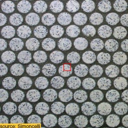 Figure 2
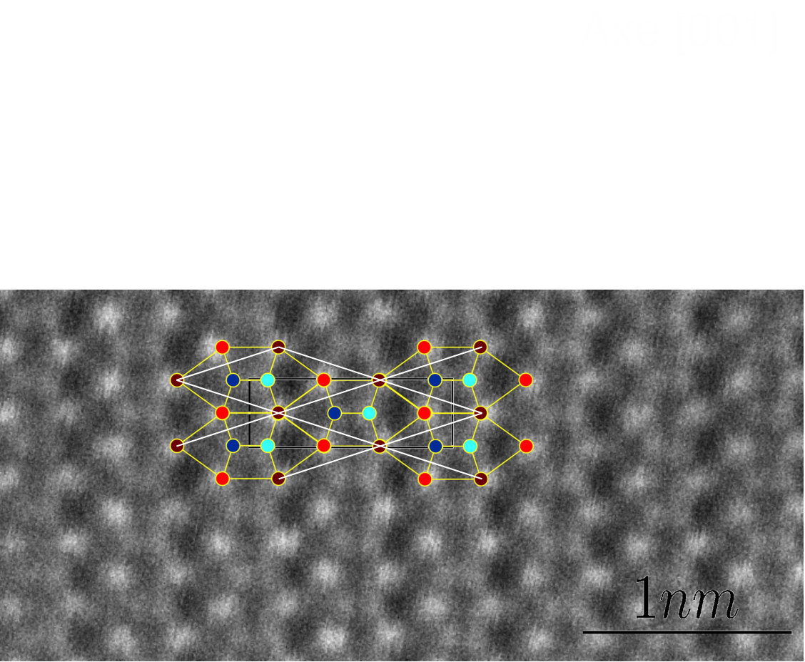 Figure 3
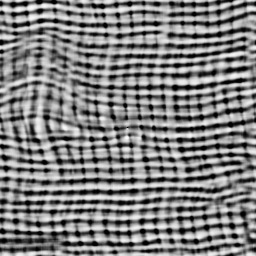 Figure 4
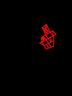 Figure 5
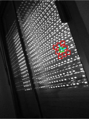 Figure 6
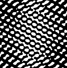 Figure 7
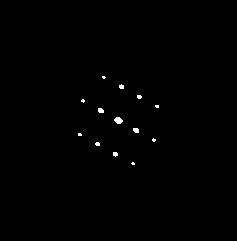 Figure 8
 Figure 9
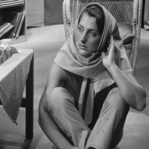 Figure 10
 Figure 11
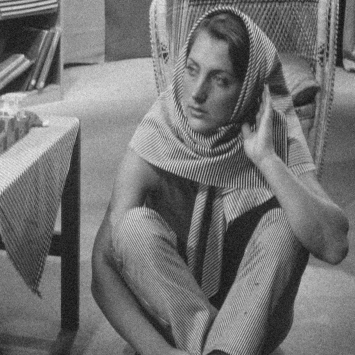 Figure 12
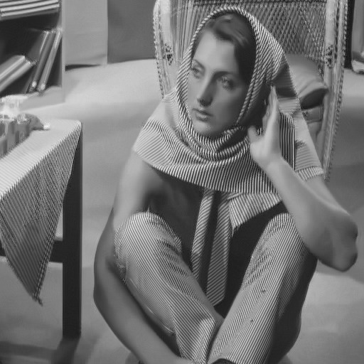 Figure 13
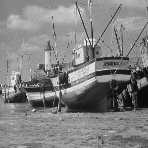 Figure 14
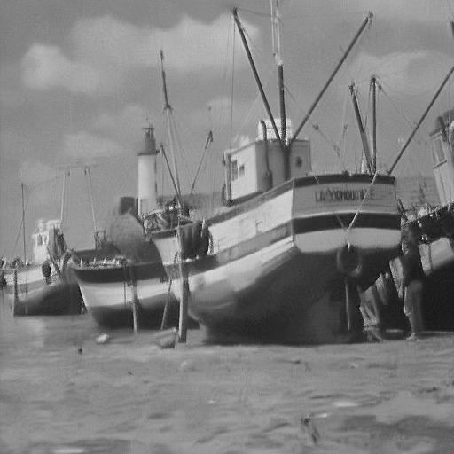 Figure 15
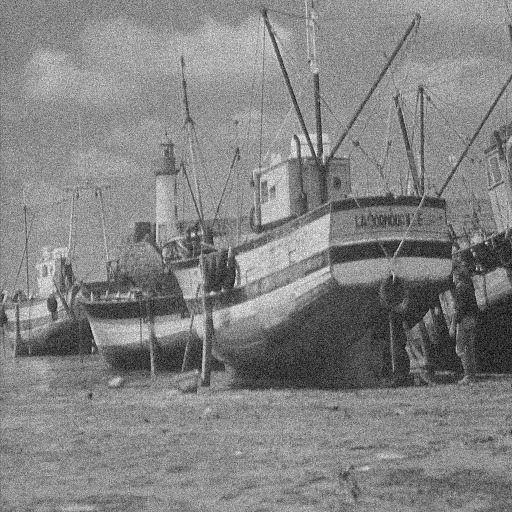 Figure 16
 Figure 17
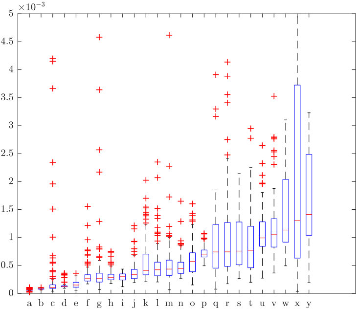 Figure 18
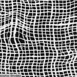 Figure 19
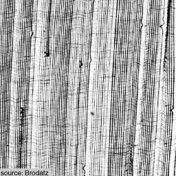 Figure 20
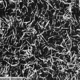 Figure 21
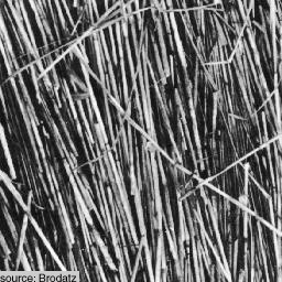 Figure 22
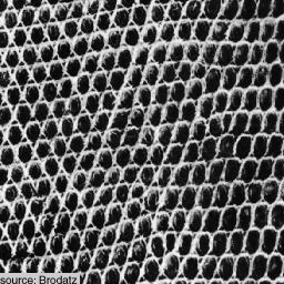 Figure 23
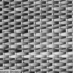 Figure 24
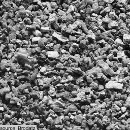 Figure 25
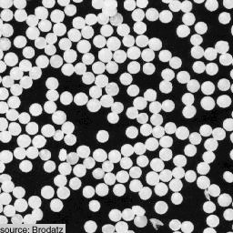 Figure 26
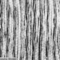 Figure 27
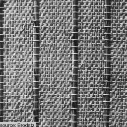 Figure 28
 Figure 29
 Figure 30
 Figure 31
 Figure 32
 Figure 33
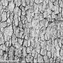 Figure 34
 Figure 35
 Figure 36
 Figure 37
 Figure 38
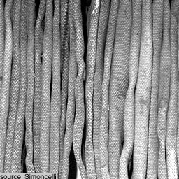 Figure 39
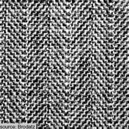 Figure 40
Peer Reviews
No public reviews on file for this paper yet. If you reviewed it on a platform where reviews are public (OpenReview, ICLR, NeurIPS, ICML), you can paste yours below so the community can read it here.
Videos
No videos yet. Explain this paper in a talk, walkthrough, or lecture? Add one.
Taxonomy
TopicsMedical Image Segmentation Techniques · Image Retrieval and Classification Techniques · Cell Image Analysis Techniques
Patch redundancy in images: a statistical testing framework and some applications
Valentin De Bortoli
CMLA, ENS Cachan, CNRS, Université Paris-Saclay, 94235 Cachan, France
&Agnès Desolneux
CMLA, ENS Cachan, CNRS, Université Paris-Saclay, 94235 Cachan, France
&Bruno Galerne
Institut Denis Poisson, Université d’Orléans, Université de Tours, CNRS
&Arthur leclaire
Univ. Bordeaux, IMB, Bordeaux INP, CNRS, UMR 5251, F-33400 Talence, France.
Abstract
In this work we introduce a statistical framework in order to analyze the spatial redundancy in natural images. This notion of spatial redundancy must be defined locally and thus we give some examples of functions (auto-similarity and template similarity) which, given one or two images, computes a similarity measurement between patches. Two patches are said to be similar if the similarity measurement is small enough. To derive a criterion for taking a decision on the similarity between two patches we present an a contrario model. Namely, two patches are said to be similar if the associated similarity measurement is unlikely to happen in a background model. Choosing Gaussian random fields as background models we derive non-asymptotic expressions for the probability distribution function of similarity measurements. We introduce a fast algorithm in order to assess redundancy in natural images and present applications in denoising, periodicity analysis and texture ranking.
K****eywords patch, redundancy, statistical framework, a contrario method, image denoising, texture, periodicity analysis.
1 Introduction
In many image processing applications, using local information combined with the knowledge of long-range spatial arrangement is crucial. The spatial redundancy on sub-images called patches, encodes the small scale structure of the image as well as its large scale organization. More precisely, local information is encoded in the patch content and the large scale organization is contained in the redundancy of this information across the patches of the image. For example, patch-based inpainting techniques, such as [10, 33], assign patches of a known region to patches of an unknown region. Namely, each patch position on the border of the unknown region is associated to an offset corresponding to the best patch according to the partial available information. In [33] the authors replace the search on the whole image by a search among the most redundant offsets in the known region. This allows the authors of [33] to retrieve long-range spatial structure in the unknown part of the image. Another famous application of spatial redundancy can be found in denoising, with the seminal work (Non-Local means) of Buades and coauthors [5], in which the authors propose to replace a noisy patch by the mean over all spatially redundant patches.
Last but not least, spatial redundancy is of crucial importance in exemplar-based texture synthesis. In this paper we define textures as images containing repeated patterns but also reflecting randomness in the arrangement of these patterns. Among textures, one important class is given by the microtextures in which no individual object can be clearly delimited. In the periodic case, a more precise definition will be given in Definition 4. These microtexture models can be described by Gaussian random fields [62, 27, 42, 68]. Parametric models using features such as wavelet transform coefficients [55], scattering transform coefficients [59] or convolutional neural network outputs [29] have been proposed in order to derive image models with more structure. On the other hand, non-parametric patch-based algorithms such as [25, 24, 38, 56, 28] propose to use most similar patches in order to fill the new texture images, similarly to inpainting techniques.
All these techniques lift images in spaces with dimensions higher than the original image space, and make use of the redundancy of the lifting to extract important structural information. There exist two main types of lifting: feature extraction or patch extraction. Feature extraction relies on the use of filters, linear or non-linear, which aim at selecting substantial local information. Among popular kernels are oriented and multiscale filters, which happened to be identified as early processing in mammal vision systems [13, 35]. These last years have seen the rise of neural networks in which the filter dictionary is no longer given as an input but learned through a data-driven optimization procedure [60]. On the other hand, patch-based methods rely on the assumption that image processing tasks are simplified when conducted in the higher dimensional patch space.
Every analysis performed in a lifted space, built via feature extraction or patch extraction, relies on the comparison of points in this space. In patch-based lifted spaces, we aim at finding dissimilarity functions such that two patches are visually close if the dissimilarity measurement between them is small. In this paper we focus on the square Euclidean distance but other choices could be considered [64, 65, 15, 17].
This leads us to consider a statistical hypothesis testing framework to assess similarity (or dissimilarity) between patches. The null hypothesis is defined as the absence of local structural similarities in the image. Reciprocally the alternative hypothesis is defined as the presence of such similarities. There exists a wide variety of tractable models exhibiting no similarity at long-range, like Gaussian random fields [62, 27, 42, 68] or spatial Markov random fields [11], whereas sampling and inference in very structured models rely on optimization procedures and may be computationally expensive, their distribution being the limit of some Markov chain [70, 47] or some stochastic optimization procedure [4]. This encourages us to consider an a contrario approach, i.e. we do not consider the alternative hypothesis and focus on rejecting the null hypothesis. This framework was successfully applied in many areas of image processing [14, 19, 20, 1, 7] and aims at identifying structure events in images. This statistical model takes its roots in the fundamental work of the Gestalt theory [21]. One of its principle, the non-accidentalness principle [46] or Helmholtz principle [69, 20], states that no structure is perceived in a noise model. To be precise, in our case of interest, we want to assess that no spatial redundancy is perceived in microtexture models. This methodology allows us to only design a locally structured background model to define a null hypothesis. Combining a contrario principles and patch-based measures, we propose an algorithm to identify auto-similarities in images.
We then turn to the implementation of such an algorithm and illustrate the diversity of its possible applications with three examples: denoising, lattice extraction, and periodicity ranking of textures. In our denoising application we propose a modification of the celebrated Non-Local means algorithm [5] (NL-means) by inserting a threshold in the selection of similar patches. Using an a contrario model we are able to give probabilistic control on the patch reconstruction.
We then focus on periodicity detection and, more precisely, lattice extraction. Periodicity in images was described as an important feature in early mathematical vision [32]. Most of the proposed methods to analyze periodicity rely on global measurements such as the modulus of the Fourier transform [49] or the autocorrelation [43]. These global techniques are widely used in crystallography where lattice properties, such as the angle between basis vectors, are fundamental [50, 58]. Since all of our measurements are local, we are able to identify periodic similarities even in images which are not periodic but present periodic parts, for instance if two crystal structures are present in a single crystallography image. We draw a link between the introduced notion of auto-similarity and the inertia measurement in co-occurence matrices [32]. We then introduce our lattice proposal algorithm which combines a detection map, i.e. the output of our redundancy detection algorithm, and graphical model techniques, as in [53], in order to extract lattice basis vectors.
Our last application concerns texture ranking. Since the definition of texture is broad and covers a wide range of images, it is a natural question to identify criteria in order to distinguish textures. In [45], the authors use a classical measure for distinguishing textures: regularity. In this work, we narrow this criterion and restrict ourselves to the study of periodicity in texture images. The proposed graphical model inference naturally gives a quantitative measurement for texture periodicity ranking. We give an example of ranking on 25 images of the Brodatz set.
Our paper is organized as follows. An a contrario framework for local similarity detection is proposed in Section 1. In the a contrario framework, a background model, corresponding to the null hypothesis, is required. The consequence of choosing Gaussian models as background models is investigated and a redundancy detection algorithm is proposed in Section 3. The rest of the paper is dedicated to some examples of application of the proposed framework. After reviewing one of the most popular method in image denoising we introduce a denoising algorithm in Section 4.1 and present our experimental results in Section 4.2. Local dissimilarity measurements can be used as periodicity detectors. The link between the locality of the introduced functions and the literature on periodicity detection problems is investigated in Section 5.1. An algorithm for detecting lattices in images is given in Section 5.2 and numerical results are presented in Section 5.3. In our last experiment in Section 5.4, we introduce a criterion for measuring texture periodicity. We conclude our study and discuss future work in Section 6.
2 An a contrario framework for auto-similarity
We first introduce a notion of dissimilarity between patches of an input image.
Definition 1** (Auto-similarity)**
Let be an image defined over a domain , with . Let be a patch domain. We introduce the patch at position in the periodic extension of to , denoted by . We define the auto-similarity with patch domain and offset by
[TABLE]
The auto-similarity computes the distance between a patch of defined on a domain and the patch of defined by the domain shifted by the offset vector .
In what follows, we introduce an a contrario framework on the auto-similarity. This framework will allow us to derive an algorithm for detecting spatial redundancy in natural images.
In this section we fix an image domain and a patch domain . We recall that our final aim is to design a criterion that will answer the following question: are two given patches similar? This criterion will be given by the comparison between the value of a dissimilarity function and a threshold . We will define the threshold so that few similarities are identified in the null hypothesis model, i.e. similarity does not occur “just by chance”. Thus we can reformulate the initial question: is the similarity output of a dissimilarity function between two patches small enough? Or, to be more precise, how can we set the threshold in order to obtain a criterion for assessing similarity between patches?
This formulation agrees with the a contrario framework [21] which states that geometrical and/or perceptual structure in an image is meaningful if it is a rare event in a background model. This general principle is sometimes called the Helmholtz principle [69] or the non-accidentalness principle [46]. Therefore, in order to control the number of similarities identified in the background model, we study the probability density function of the auto-similarity function with input random image over . We will denote by the probability distribution of over , the images over . We will assume that is a microtexture model, see Definition 4 below for a precise definition of such a model. We define the following significant event which encodes spatial redundancy: , where , the threshold function, is defined over the offsets () but also depends on other parameters such as or . The dependency of with respect to cannot be omitted. For instance, even in a Gaussian white noise , the probability distribution function of depends on .
The Number of False Alarms () is a crucial quantity in the a contrario methodology. A false alarm is defined as an occurrence of the significant event in the background model . We recall that in our model the significant event is patch redundancy. This test must be conducted for every possible configurations of the significant event, i.e. in our case we test every possible offset . The is then defined as the expectation of the number of false alarms over all possible configurations. Bounding the ensures that the probability of identifying offsets with spatial redundancy is also bounded, see Proposition 1. In what follows we give the definition of the in the spatial redundancy context.
Definition 2** ()**
Let , where is a background microtexture model. We define the auto-similarity probability map for any , and by
[TABLE]
We define the auto-similarity expected number of false alarms by
[TABLE]
Note that corresponds to the probability that is similar to in the background model . For any , the cumulative distribution function of the auto-similarity random variable under evaluated at value is given by . We denote by the inverse cumulative distribution function, potentially defined by a generalized inverse (), of the auto-similarity random variable for a fixed offset , with a quantile. We now have all the tools to control the number of detected offsets in the background model.
Definition 3** (Detected offset)**
Let be an image, a patch domain, and . An offset is said to be detected with respect to , if .
Note that a detected offset in corresponds to a false alarm in the a contrario model. In what follows we suppose that the cumulative distribution function of is invertible for every . This ensures that for any and we have
[TABLE]
Proposition 1
Let and for all define . We have that for any ,
[TABLE]
Proof:
Using (3), and , we get
[TABLE]
where the last equality is obtained using (4). Concerning the upper-bound, we have, using the Markov inequality and (2), for any
[TABLE]
where if and [math] otherwise.
Thus, setting as in Proposition 1, we have that an offset is detected for an image if
[TABLE]
This a contrario detection framework can then be simply rewritten as 1) computing the auto-similarity function with input image , 2) thresholding the obtained dissimilarity map with the inverse cumulative distribution function of the computed dissimilarity function under . The computed threshold depends on the offset and Proposition 1 ensures probabilistic guarantees on the expected number of detections under . Using the inverse property of the inverse cumulative distribution function and (5), we obtain that an offset is detected if and only if
[TABLE]
Therefore, the thresholding operation can be conducted either on , see (5), or on , see (6). This property will be used in Section 3.2 to define a similarity detection algorithm based on the evaluation of .
3 Gaussian model and detection algorithm
3.1 Choice of background model
In this section we compute , i.e. the cumulative distribution function of the similarity function under the null hypothesis model, with a Gaussian background model. Indeed, if the background model is simply a Gaussian white noise the similarities identified by the a contrario algorithm are the ones that are not likely to be present in the Gaussian white noise image model. More generally, we consider stationary Gaussian random fields defined in the following way: we introduce an image over which contains the microtexture information we want to discard in our a contrario model. In what follows we give the definition of the microtexture model associated to .
Definition 4** (Microtexture model)**
Let , we define the associated microtexture model by setting, , where is the periodic convolution operator over given by and is a white noise over , i.e. are i.i.d. random variables.
Given an image , a microtexture model can be derived considering
[TABLE]
Note that if is given by (7) we have for any
[TABLE]
We refer to [27] for a mathematical study of this model.
3.2 Detection algorithm
In this section, is a finite square domain in . We fix . We also define , a function over . We consider the Gaussian random field , where is a Gaussian white noise over . We denote by the autocorrelation of , i.e. where for any , . We introduce the offset correlation function defined for any by
[TABLE]
The following proposition, proved in [15], gives the explicit probability distribution function of the squared auto-similarity.
Proposition 2** (Squared auto-similarity function exact probability distribution function)**
Let with , , and where is a Gaussian white noise over . Then, for any , has the same distribution as , with independent chi-square random variables with parameter 1 and the eigenvalues of the covariance matrix associated with function restricted to , defined in (9), i.e for any , .
As a consequence if , i.e. is a Gaussian white noise, and , i.e. there is no overlapping between the patch domain and its shifted version, then is a chi-square random variable with parameter .
In order to compute the cumulative distribution function of a quadratic form of Gaussian random variables we must deal with two issues: 1) the computation of the eigenvalues might be time-consuming and efficient methods must be developed ; 2) the exact computation of the cumulative distribution function of a quadratic form of Gaussian random variables requires the use of heavy integrals, see [36]. In [15] a projection method is introduced in order to easily compute approximated eigenvalues, with equality when . The so-called Wood F method (see [66, 3]) shows the best trade-off between accuracy and computational cost to approximate the cumulative distribution function of quadratic forms in Gaussian random variables with given weights. It is a moment method of order 3, fitting a Fisher-Snedecor distribution to the empirical one. Note that in [44] another moment method of order 3 is proposed. In what follows, we assume that we can compute the cumulative distribution function of and we refer to [15] for further details.
In Algorithm 1 we propose an a contrario framework for spatial redundancy detection. We suppose that and are provided by the user. Using Proposition 1 and (6) , we say that an offset is detected if . The value is supposed to be set by the user. The background model used in the auto-similarity detection is the one given in (7). Therefore, Proposition 2 and the discussion that follows can be used to compute an approximation of . In Figure 2 we apply Algorithm 1 to a texture image.
4 Denoising
4.1 NL-means and a contrario framework
In this section we apply the a contrario framework to the context of image denoising and propose a simple modification of the celebrated image denoising algorithm Non-Local Means (NL-means). This algorithm was introduced in the seminal paper of Buades et al. [5] and was inspired by the work of Efros and Leung in texture synthesis [25]. It was also independently introduced in [2]. This algorithm relies on the simple idea that denoising operations can be conducted in the lifted patch space. In this space the usual Euclidean distance acts as a good similarity detector and we can obtain a denoised patch by averaging all the patches with weights that depend on this Euclidean distance. Usually the weight function is set to have exponential decay, but it was suggested in [30, 57, 22] to use compactly supported weight functions in order to avoid the loss of isolated details. Since its introduction, many algorithms derived from NL-means have been proposed in order to embed the algorithm in general statistical frameworks [23, 41] or to take into account the underlying geometry of the patch space [34]. Among the state-of-the-art denoising algorithms, see [39] for a review, we consider Block-Matching and 3D Filtering (BM3D) [12] to compare our algorithm with.
There exist several works combining a contrario models and denoising tasks. Coupier et al. in [9] propose to combine morphological filters and a testing hypothesis framework to remove impulse noise. In [18] Delon and Desolneux compare different statistical frameworks to perform denoising with Gaussian noise or impulse noise. The a contrario model was also successfully used to deal with speckle noise [26] and quasi-periodic noise [61], and rely on the thresholding of wavelet or Fourier coefficients. In [37], Kervrann and Boulanger derive approximated probabilistic thresholds using probability distribution functions. In [67] the authors propose a testing framework in order to estimate thresholds. The expressions they derive also relies on an approximation of the probability distribution of the squared Euclidean norm between two patches in Gaussian white noise.
Following a standard extension procedure of the NL-means algorithm we consider a threshold version of it, see Algorithm 2. In what follows we fix a “clean”, or original, image defined over , a finite rectangular domain of , a noisy image , with a realization of a standard Gaussian random field and the standard deviation of the noise. In all of our experiments we suppose that is known. Note that there exist several algorithms to estimate from real images, see [54] for instance. Our goal is to retrieve based on the information in . We consider the lifted version of in a patch space. Let be a centered patch domain. For a patch window the patch search window will be defined by
[TABLE]
with . denotes the cardinality of . There exists a large literature concerning the setting of and , see [22]. Note that the locality of the patch window was assessed to be a crucial feature of NL-means [31]. Suppose we have a collection of denoised patches for all patch domains , we obtain a pixel at position in the denoised image using the following average, see [6],
[TABLE]
We now introduce our modification of NL-means. We suppose that we are provided a threshold function . The choice of such a function is discussed in Proposition 3.
Note here that the output denoised version of the patch verifies the following equation
[TABLE]
In the original NL-means method, we have
[TABLE]
Setting is not trivial and depends on many parameters (patch size, search window size, content of the original image). As in Algorithm 2, we denote . The following proposition, similar to Proposition 1, gives a method for setting . We say that an offset is a false alarm in a Gaussian white noise if the associated patch is not used in the denoising algorithm. In Proposition 3 we choose in order to control the number of false alarms with high probability.
Proposition 3
Let , given in (10) and let be defined for any by
[TABLE]
with background model being a Gaussian white noise , i.e. in Definition 4. Let be defined in (10) and the random number of selected patches used to denoise the patch , see Algorithm 2. Then for any it holds that
[TABLE]
Proof:
Using the Markov inequality, we have
[TABLE]
In this case the null hypothesis is given by a standard Gaussian random field, which is a special case of the Gaussian random field models introduced in Section 3. In the next proposition, using the a contrario framework, we obtain probabilistic guarantees on the distance between the reconstructed patch and the true patch .
Proposition 4
Let , where is a standard Gaussian white noise over , and . Let and be a fixed patch and let . We introduce the random set (the selected offsets) with as in Proposition 3 and defined in (10). Let . Then for any , setting , we have
[TABLE]
Proof:
We have for any
[TABLE]
This gives the following event inclusion for any ,
[TABLE]
We also have that by definition of
[TABLE]
In our applications we use Algorithm 2 with . Therefore we need to compute with a Gaussian white noise background model. We recall that in Section 3.2, using Proposition 2, we give a method to compute this quantity in general Gaussian settings. In the case of a Gaussian white noise, the next proposition shows that the eigenvalues can be computed without approximation.
Proposition 5
Let , as in Proposition 2 with and , with . We have, expressing in the basis corresponding to the raster scan order on the -axis
[TABLE]
where is a zero matrix with ones on the -th diagonal. The eigenvalues of are given by with multiplicity where , and . For any , it holds
- (a)
for any , 2. (b)
** 3. (c)
** 4. (d)
**
with , where . We define in the same manner. A similar proposition holds if .
Proof:
The proof is postponed to Appendix A.
This property allows us to compute exactly the eigenvalues appearing in Proposition 2. In Figure 3 we illustrate that for fixed patch size () and patch search window (). Thus in our implementation we suppose that is constant and set its value to the mean of over .
4.2 Some experimental results
In the following paragraph we present and comment some results of our threshold NL-means algorithm, see Algorithm 2. We recall that we use . In Figure 4 we present a first comparison with the NL-means algorithm. Perceptual results as well as Peak Signal to Noise Ratio () measurements 111 are commented. We also present the running time of the original NL-means algorithm and ours. The experiments were conducted with the following computer specifications: 16G RAM, 4 Intel Core i7-7500U CPU (2.70GHz). Results on other images than Barbara are displayed in Figure 5.
If the threshold is high, i.e. then almost no patch is rejected, which means that almost all patches are used in the denoising process. In consequence, the output denoised image is very smooth. This smoothness is a correct guess for constant patches. However, this proposition does not hold when the region contains details. Indeed, in this case details are lost due to the averaging process. By setting a conservative threshold, e.g. , for example, we reject all the patches for which the structure does not strongly match the one of the input patch, see Figure 6. This conservative property of the algorithm ensures that we can control the loss of information in the denoised image, see Proposition 4. However, if no patch, other than the input patch itself, is detected as similar we highly overfit the original noise. Many algorithms such as BM3D, see [12], solve this problem by treating this case as an exception, applying a specific denoising method in this situation. We show the differences between our version of NL-means and BM3D in Figure 7 .
In Figure 8, we show that Algorithm 2 performs better than the original NL-means algorithm. By setting we obtain that the of the denoised image is better than the one of NL-means for nearly every value of .
Let us emphasize that our goal is not to provide a new state-of-the-art denoising algorithm. Indeed we never obtain better denoising results than the BM3D algorithm. However, our algorithm slightly improves the original NL-means algorithm. It shows that statistical testing can be efficiently used to measure the similarity between patches and therefore provides a robust way to perform the weighted average in this algorithm.
5 Periodicity analysis
5.1 Existing algorithms
In the following sections we use our patch similarity detection algorithm, see Algorithm 1, to analyze images exhibiting periodicity features. Let be a finite domain and a finite patch domain.
Periodicity detection is a long-standing problem in texture analysis [71]. First algorithms used the quantization of images, relying on co-occurrence matrices and statistical tools like tests or tests. Global methods extract peaks in the frequency domain (Fourier spectrum) [49] or in the spatial domain (autocorrelation). In [32] the notion of inertia is introduced. It is defined for any by , where is a quantized image on gray levels. In [8], the authors show that the local minima of the inertia measurement can be used to assess periodicity. Similarly, we introduce the -inertia for any by . The following proposition extends to a local framework results from [52].
Proposition 6
Let . Suppose that is quantized, i.e. there exists such that for any , . We have .
Proof:
For any we have
[TABLE]
If then the -inertia statistics is exactly the inertia introduced in [32] and the result is due to [52].
5.2 Algorithm and properties
Lattice detection is closely related to periodicity analysis, since identifying a lattice is similar to extracting periodic or pseudo-periodic structures up to deformations and approximations. A state-of-the-art algorithm proposed in [53] uses a recursive framework which consists in 1) a lattice model proposal based on detectors such as Kanade-Lucas-Tomasi () feature trackers [48], 2) spatial tracking using inference in a probabilistic graphical model, 3) spatial warping correcting the lattice deformations in the original image. In this section we propose a new algorithm for lattice detection. The lattice proposal step 1) is replaced by an Euclidean auto-similarity matching detection (see Section 3.2 and Algorithm 1) where the patch domain is fixed. Using these detections we build a graph with a few nodes (usually approximately nodes for a image). We use the same notation for the detection mapping i.e. the output of Algorithm 1, which is a binary function over the offsets, and the set of detected offsets. We recall that two pixel coordinates and are said to be -connected if with . The graph is then built as follows:
Vertices: for each 8-connected component, in we note one position for which the minimum of over is achieved. The set of vertices is defined as where is the number of 8-connected components in ;
Edges: each vertex is linked with its four nearest neighbors in the sense of the Euclidean distance, defining four unoriented edges.
Refering to the three steps of [53] we present our model to replace step 2) (i.e. the inference in a probabilistic graphical model) and introduce the approximated lattice hypothesis defined on a graph.
Definition 5** (Approximated lattice hypothesis)**
Let be a random graph with . We say that follows the approximated lattice hypothesis if there exists a basis of and, for each edge , a couple of integers such that has the same distribution as , with independent standard Gaussian random variables in and . We denote by the vector of all coefficients .
Our goal is to perform inference in the statistical model defined by the following log-posterior
[TABLE]
where with . A discussion on the dependence of the model on the hyperparameters is conducted in Figure 9. Finding the of this full log-posterior is a non-convex, integer problem. However performing the minimization alternatively on and is easier since at each step we only have a quadratic function to minimize. Minimizing a positive-definite quadratic function over is equivalent to finding the vector of minimum norm in a lattice. This last formulation is known as the Shortest Vector Problem () which is a challenging problem [51] (though it is not known if it is a -hard problem). We replace this minimization procedure over a lattice by a minimization over followed by a rounding of this relaxed solution.
For any we denote by , with , the log-posterior sequence.
Proposition 7** (Alternate minimization update rule)**
In Algorithm 3, we get for any
[TABLE]
with the tensor product between matrices and
- (a)
** 2. (b)
**
Proof:
The proof is postponed to Appendix B.
Note that if is orthogonal, i.e. then is diagonal and the proposed method is the exact solution to the minimization problem over .
Theorem 1** (Convergence in finite time)**
For any , is a non-decreasing sequence. In addition, and converge in a finite number of iterations.
Proof:
is non-decreasing since for any , . Let us show that the sequences and are bounded. Because is non-decreasing, the sequence is non-increasing. We obtain that
[TABLE]
The sequence is bounded thus we can extract a converging subsequence. Since takes value in , this subsequence is stationary with value . Let be the first time we hit value . Let , with , there exists , with such that thus
[TABLE]
Hence for every , . Suppose there exists such that this means that (because of lines 6 and 7 of Algorithm 3) which is absurd. Thus is stationary and so is .
In Algorithm 3 is initialized with zero and is defined as an orthonormal (up to a dilatation factor) direct basis where the first vector is given by an edge with median norm in .
5.3 Experimental results
Combining the results of Section 5.2 and Section 3.2 we obtain an algorithm to extract lattices in images, see Figure 10. In what follows we perform lattice detection using Algorithm 1 in order to extract auto-similarity given a patch in an original image , which implies that the patch domain is set by the user. Recall that in Algorithm 1, the eigenvalues of the covariance matrix in Proposition 2 are approximated, and that the cumulative distribution function of the quadratic form in Gaussian random variables is computed via the Wood F method [66]. Lattice detection is performed using Algorithm 3 with parameters and .
5.3.1 Escher paving
In this section we study art images, Escher pavings, with strongly periodic structure. We investigate the following parameters of our lattice detection algorithm:
- (a)
background microtexture model , 2. (b)
parameter in Algorithm 1, 3. (c)
patch domain .
Microtexture model
We confirm that the choice of the microtexture model will influence the detected geometrical structures. The more structured is the background noise model the less we obtain detections. This situation is considered in Figure 11.
parameter
Using a more adapted microtexture model as background model we gain robustness compared to other less structured models such as a Gaussian white noise. However, must be set carefully otherwise two situations can occur:
- (a)
if is too high, too many detections can be obtained (true perceptual detections are not differentiated from false positives) ; 2. (b)
if is too low, we fail to identify important perceptual structures in the image.
We observe that a general good practice is to set equal to , see Figure 12. However, if the input patch is corrupted one may increase this parameter up to or , see Figure 17 and Figure 18.
Patch position
Patch position and size are crucial in our detection model, since we rely on local properties of the image. As shown in Figure 13 these parameters should be carefully selected by the user. However, for particular applications such as lattice extraction for crystallographic purposes, there exist procedures to extract primitive cells [50].
5.3.2 Crystallography images
Defect localization, noise reduction, correction of crystalline structures in images are central tasks in crystallography. Usually, they require the knowledge of the geometry of a perfect underlying crystal. In our experiments we manually identify the geometry of the periodic crystal, which allows for multiple structures in one image, provided a user input of the primitive cell in a lattice. This primitive cell extraction could be automated [50]. In Figure 14, we present an example of multiple geometry extraction. Statistics like angle and period can be retrieved using the estimated basis vectors. This image contains two lattices and the locality of our measurements allows for the detection of both structures. Using windowed Fourier transform could be efficient to obtain local measurements on the periodicity of these images since the information is highly frequential. However in order to obtain the same detection map as Algorithm 1 one must carefully set the threshold parameter, . This situation is illustrated in Figure 15.
Finally we assess the precision of our measurements by comparing our results with a model used in crystallography, see Figure 16. We indeed retrieve one of the possible bases used to describe these lattices. However, the symmetry constraints are not present in the identified basis. To obtain another basis, one must relax the regularization parameters. A more natural way to obtain the desired primitive cell would be to introduce symmetry constraints in the graphical model formulation in (14).
5.3.3 Natural images
Identifying lattices in natural images is a more challenging task since we have to deal with image artifacts. In this section we investigate the effect on the detection of the background clutter in natural images, see Figure 17, and the effect of the camera position, see Figure 18.
Preprocessing
Due to the occlusions occurring in natural images, if a lattice is superposed over a real photograph, carefully selecting structural elements might not be enough in order to retrieve the periodicity. Indeed, if we observe a repetition of the lattice pattern, the background does not necessarily contain any repetition and thus makes the detection more complicated. In order to avoid such a problem we propose to introduce a preprocessing step in our algorithm. This preprocessing step will be encoded in a linear filter . Suppose is a sample from a Gaussian model with function then is a sample from a Gaussian model with function . Thus all the properties derived earlier remain valid with this linear operation. In Figure 17, we set to be a Laplacian operator 222We use a discrete Laplacian operator such that for any , we get that , where boundaries are handled periodically.. This operation allows us to avoid contrast problems.
Homography
In the previous experiments we suppose that the lattice structure was in front of the camera. In many cases this assumption is not true and there exists an homography that matches the deformed lattice in the image to a true lattice. Our algorithm makes the assumption that the lattice is viewed in a frontal way and fails otherwise. However, locally, this assumption is true and we can observe partial match of the lattices in Figure 18.
5.4 Texture ranking
We conclude these experiments by showing that this simple graphical model can be used to perform ranking among texture images, sorting them according to their degree of periodicity. We say that an image has high periodicity degree if a lattice structure can be well fitted to the image. We introduce a criterion for evaluating the relevance of the lattice hypothesis. Let be an image over , let be a patch domain and be as in Proposition 1 with set by the user.
Definition 6** (Periodicity criterion)**
Let be the set of detected offsets and its number of connected components as defined in Section 5.2. Let also be the estimated parameters using Algorithm 3. We define the following periodicity criterion as
[TABLE]
where .
The criterion simply computes the ratio between the error area of Algorithm 3, i.e. the error made when considering the approximated lattice hypothesis, see Definition 5, and the area of the parallelogram defined by the output basis vectors. If we have enough detections this quantity is supposed to be small when the approximated lattice hypothesis holds and large when it does not. Nonetheless, we introduce a dependency in the number of detections. Indeed, even if no lattice is perceived, the hypothesis in Definition 5 may still hold if the number of detected offsets is small.
In the experiment presented in Figure 19 we sort 25 texture images based on the criterion. Images are of size . Since the identified graph highly depends on the patch position and the patch size, for each image we uniformly sample 150 patch positions and set the patch size to . For each set of parameters we find a lattice using Algorithm 1 and Algorithm 3 with parameters \text{\operatorname{NFA}_{\text{max}}}=1, , and . A statistical study of our ranking is presented in Figure 20. Note that, from a perceptual point of view, from (a) to (n) all textures are periodic except for (f), (j) and (k) which are examples for which our algorithm fails. However, from (o) to (y), no texture is periodic.
6 Conclusion
In this paper we introduce a statistical model, the a contrario framework, to analyze spatial redundancy in images. We propose a general algorithm for detecting redundancy in natural images. It relies on Gaussian random fields as background models and takes advantage of the links between the norm and Gaussian densities. The a contrario formulation provides us with a statistically sound way of thresholding distances in order to assess similarity between patches. In this rationale we replace the task of manually setting thresholds by the selection of a Number of False Alarms.
We illustrate our contribution with three examples in various domains of image processing. Introducing a simple modification of the NL-means algorithm we show that similarity detection (in this case, dissimilarity detection) in a theoretical a contrario framework can easily be embedded in any image denoising pipeline. For instance, the threshold we introduced could be integrated into the Non-Local Bayes algorithm [41] in order to estimate mean and covariance matrices with probabilistic guarantees. The generality of our model allows for several extensions for non-Gaussian noises [16] or to take into account the geometry of the patch space [34, 63].
Turning to periodicity detection we propose a novel graphical model using the output of Algorithm 1 in order to extract lattices from images. In this model, lattice extraction is formulated as the maximization of some log-likelihood defined on a graph. We prove the finite-time convergence of Algorithm 3. We provide image experiments illustrating the role of the hyperparameters in our study and we assess the importance of selecting adaptive Gaussian random fields as background models. We remark that the expected number of false alarms parameter is linked to the choice of the input patch and give a range of possible values for settings. We also illustrate its possible application in crystallography as it correctly identifies underlying lattices in alloys. This rationale could be used to identify symmetry groups (wallpaper groups) in alloys, following the work of [45]. Finally our method is tested on natural images where some of its limits such as perspective defect or sensitivity to occlusion phenoma are identified. It must be noted that our method could easily be extended to color images by considering -valued instead of real-valued images.
Our last application consists in giving a quantitative criterion for periodicity texture ranking. This criterion is based on the parameters estimated in Algorithm 3. Since we set our background models to be Gaussian random fields and remarking that these are good microtexture approximations we wish to explore the possibility to embed our a contrario framework in texture analysis and texture synthesis algorithms. For instance an a contrario methodology could be incorporated in the algorithm proposed by Raad et al. in [56]. Another potential direction is to look at the behavior of the introduced dissimilarity functions for more general random fields in order to handle more complex and structured situations such as parametric texture synthesis.
7 Acknowledgements
The authors would like to thank Denis Gratias for the crystallography images, Jérémy Anger for some of natural images, Axel Davy who provided an OpenCL implementation of the NL-means algorithm and Thibaud Ehret for its insights and comments on denoising algorithms.
Appendix A Eigenvalues
Proof:
[Proof of Proposition 5]
We fix with and denote . Without loss of generality we consider that and . We consider an eigenvector of . Let and the function such that for any
[TABLE]
It is clear that is in bijection with . Let , and . We define over such that
[TABLE]
Using that , we have for any
[TABLE]
This implies that for any
[TABLE]
Thus the one-dimensional vector (given by the raster-scan order on the -axis) of the restriction of is an eigenvector of associated with eigenvalue .
Using that is in bijection with we get that the number of vectors is . We show that this family of vectors is linearly-independent. Let such that
[TABLE]
Since and have different support if and only if we get that for any , . This gives that is in the kernel of the matrix . Since the sinus discrete transform is invertible we obtain that for any and , . Thus the family is a basis of eigenvectors.
We aim at computing the cardinality of . By definition, in Proposition 5, . First note that . We give the following decomposition with
[TABLE]
Note that for all we have that , with . Thus . Let . The cardinality of is the cardinality of . Let we have
[TABLE]
Since we have , hence
[TABLE]
Thus . Similarly we get that and . Thus, .
We have computed for every . In order to complete our study it only remains to compute , since can be deduced from the summability condition and from . We only compute . We remark that . Let then with and . We obtain the following equivalence
[TABLE]
Since or we obtain that the first condition is always satisfied. Thus we get
[TABLE]
Using that , we conclude the proof.
Appendix B Update rules
We derive the proof of Proposition 7.
Proof:
Computing the minimum of for fixed , respectively fixed , gives the update rule for , respectively for . We obtain that
[TABLE]
where depends only on . Similar derivation goes for and we obtain the proposed update rules.
The reference list from the paper itself. Each links out to its DOI / PubMed record.
- 1[1] Andrés Almansa, Agnès Desolneux, and Sébastien Vamech. Vanishing point detection without any A priori information. IEEE Trans. Pattern Anal. Mach. Intell. , 25(4):502–507, 2003.
- 2[2] Suyash P. Awate and Ross T. Whitaker. Unsupervised, information-theoretic, adaptive image filtering for image restoration. IEEE Trans. Pattern Anal. Mach. Intell. , 28(3):364–376, 2006.
- 3[3] Dean A. Bodenham and Niall M. Adams. A comparison of efficient approximations for a weighted sum of chi-squared random variables. Stat. Comput. , 26(4):917–928, 2016.
- 4[4] J. Bruna and S. Mallat. Multiscale Sparse Microcanonical Models. Ar Xiv e-prints , January 2018.
- 5[5] Antoni Buades, Bartomeu Coll, and Jean-Michel Morel. A non-local algorithm for image denoising. In 2005 IEEE Computer Society Conference on Computer Vision and Pattern Recognition (CVPR) , pages 60–65, 2005.
- 6[6] Antoni Buades, Bartomeu Coll, and Jean-Michel Morel. Non-Local Means Denoising. Image Processing On Line , 1:208–212, 2011.
- 7[7] Frédéric Cao. Application of the Gestalt principles to the detection of good continuations and corners in image level lines. Comput. Vis. Sci. , 7(1):3–13, 2004.
- 8[8] Richard W. Conners and Charles A. Harlow. Toward a structural textural analyzer based on statistical methods. Computer Graphics and Image Processing , 12(3):224–256, 1980.