Type Ib supernova Master OT J120451.50+265946.6: radio emitting shock with inhomogeneities crossing through a dense shell
Poonam Chandra, A. J. Nayana, Claes-Ingvar Bjornsson, Francesco, Taddia, Peter Lundqvist, Alak K. Ray, and Benjamin Shapee

TL;DR
This study presents radio observations of a Type Ib supernova revealing inhomogeneities in the shock structure crossing a dense shell, emphasizing the importance of wide-band radio data for understanding supernova emission.
Contribution
The paper provides the first evidence of inhomogeneities in the radio-emitting region of a Type Ib supernova using multi-frequency radio observations.
Findings
Inhomogeneities detected in the radio-emitting shock region.
Shock crossing through a dense shell between 47 to 87 days.
Model predicts smoothing of inhomogeneities at late times.
Abstract
We present radio observations of a Type Ib supernova (SN) Master OT J120451.50+265946.6. Our low frequency Giant Metrewave Radio Telescope (GMRT) data taken when the SN was in the optically thick phase for observed frequencies reveal inhomogeneities in the structure of the radio emitting region. The high frequency Karl G. Jansky Very Large Array data indicate that the shock is crossing through a dense shell between 47 to days. The data days onwards are reasonably well fit with the inhomogeneous synchrotron-self absorption model. Our model predicts that the inhomogeneities should smooth out at late times. Low frequency GMRT observations at late epochs will test this prediction. Our findings suggest the importance of obtaining well-sampled wide band radio data in order to understand the intricate nature of the radio emission from young supernovae.
Click any figure to enlarge with its caption.
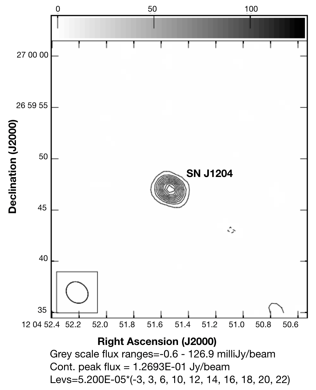 Figure 1
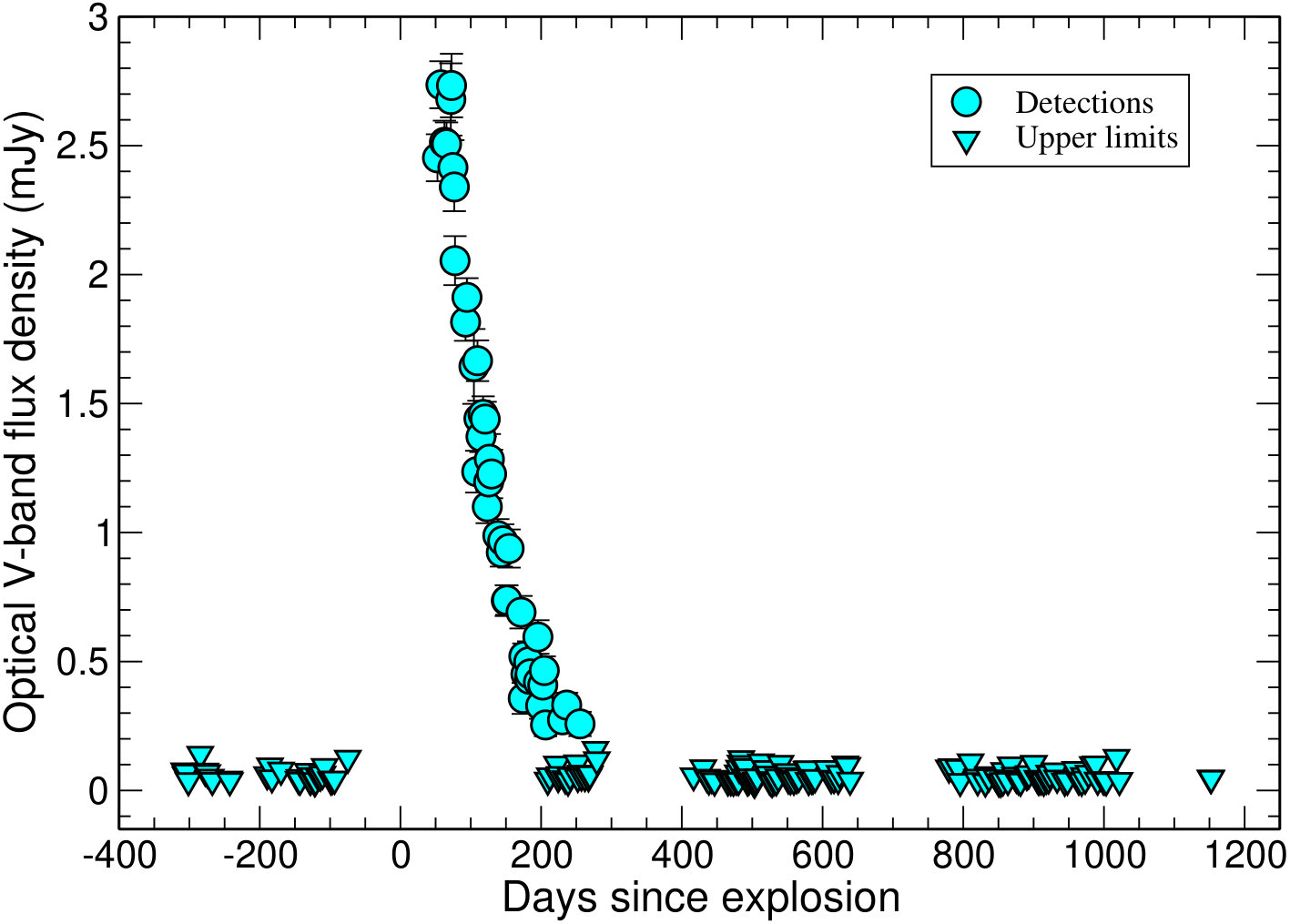 Figure 2
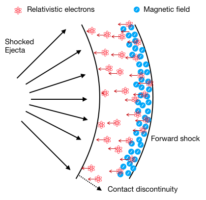 Figure 3
 Figure 4
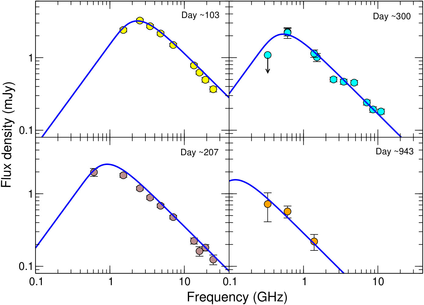 Figure 5
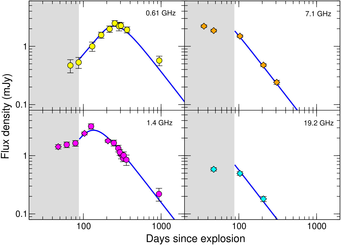 Figure 6
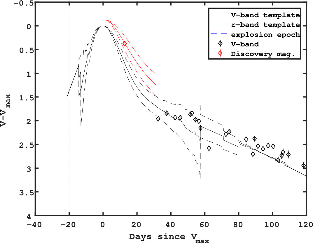 Figure 7
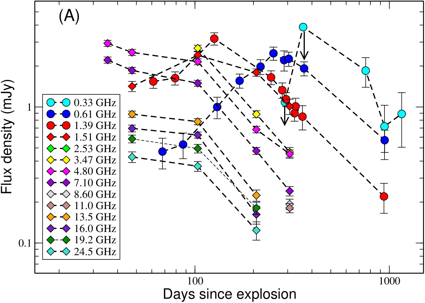 Figure 8
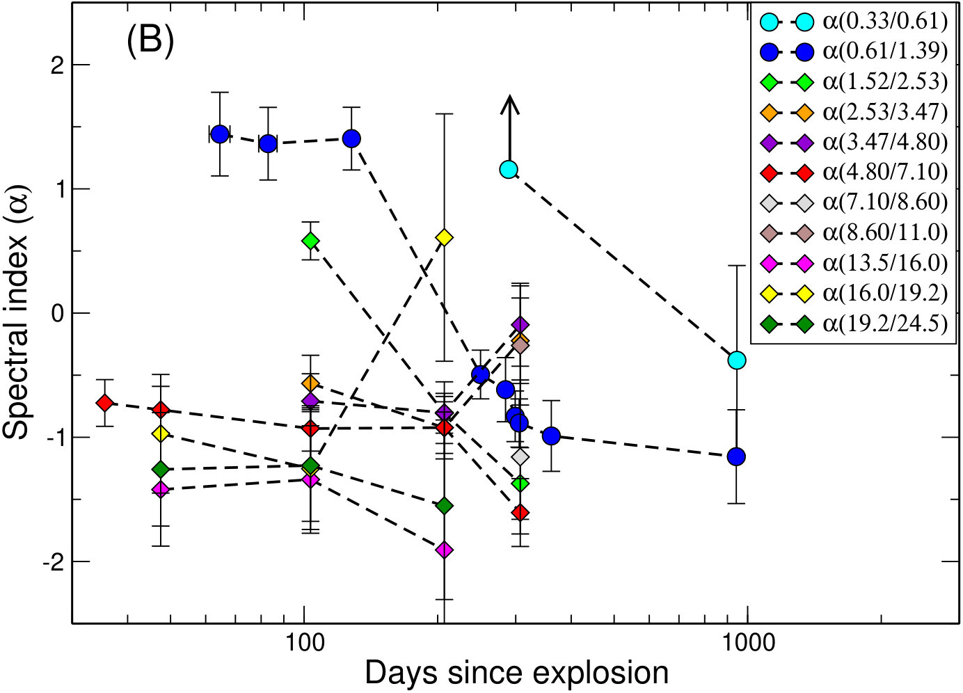 Figure 9
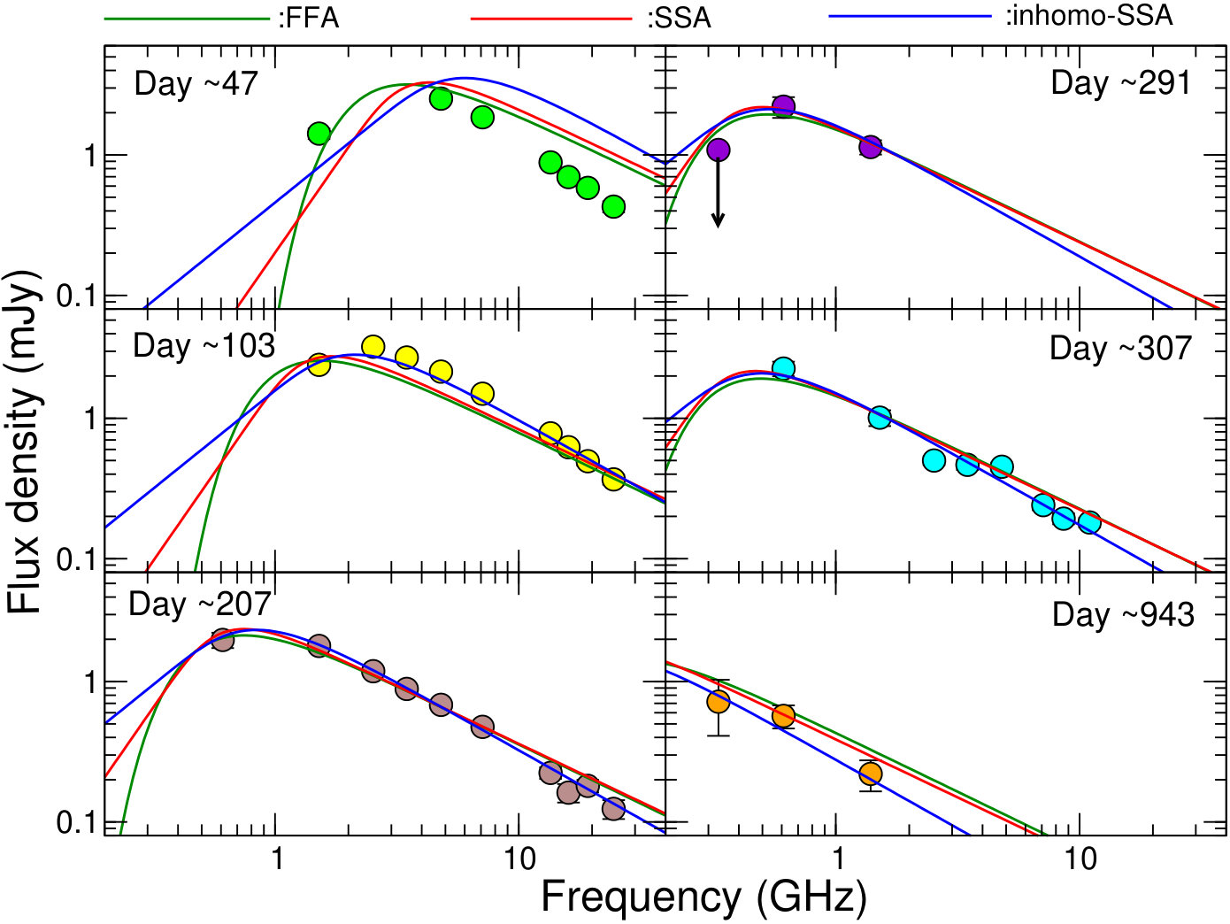 Figure 10
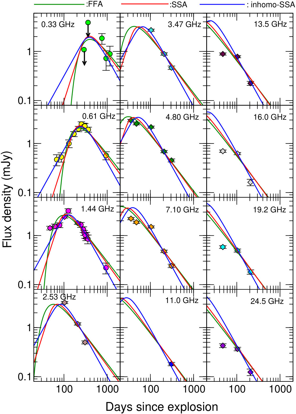 Figure 11
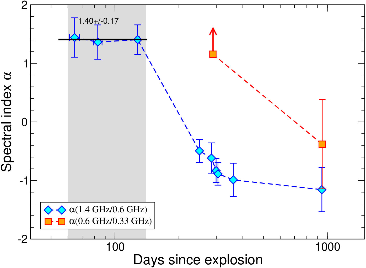 Figure 12
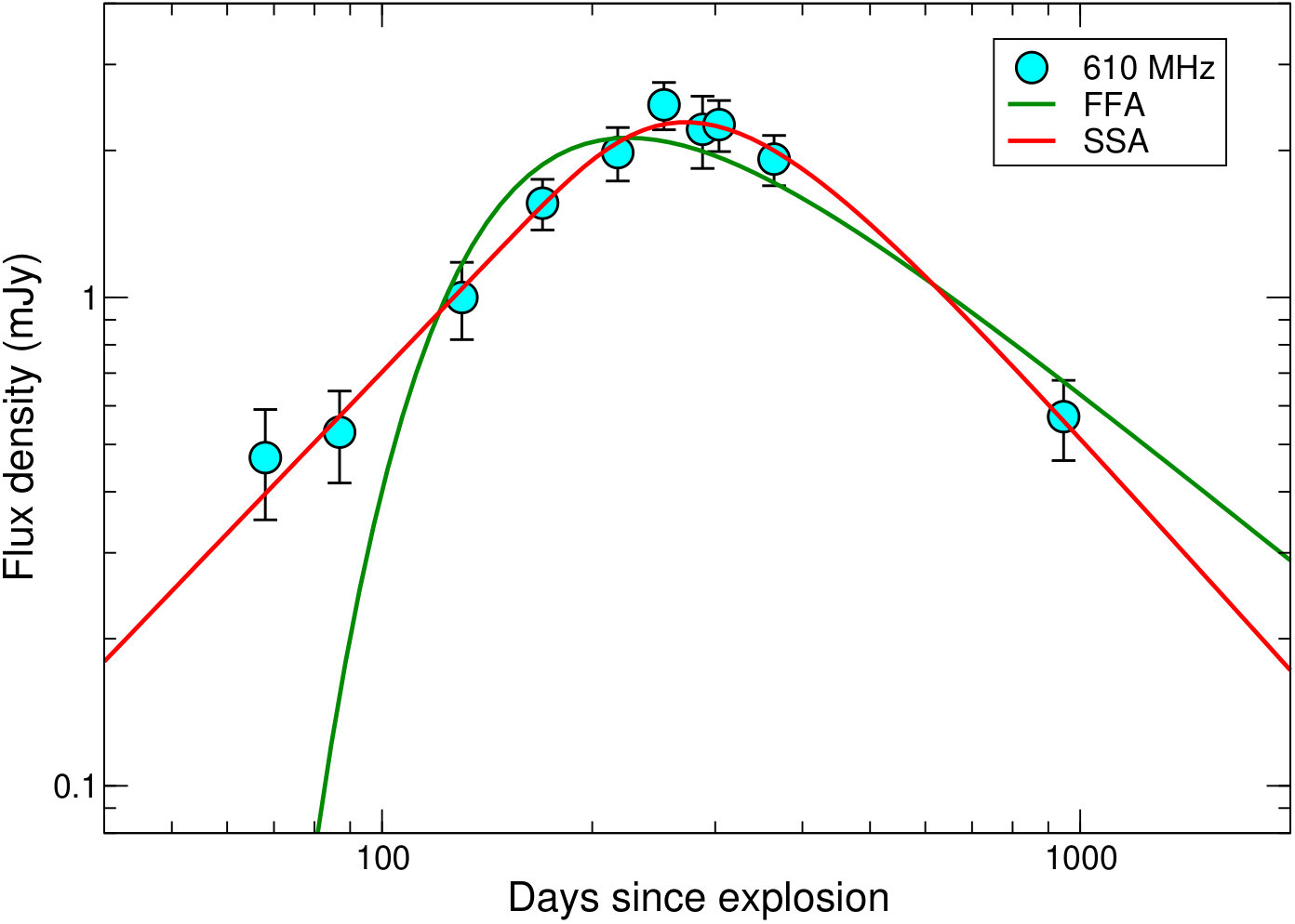 Figure 13
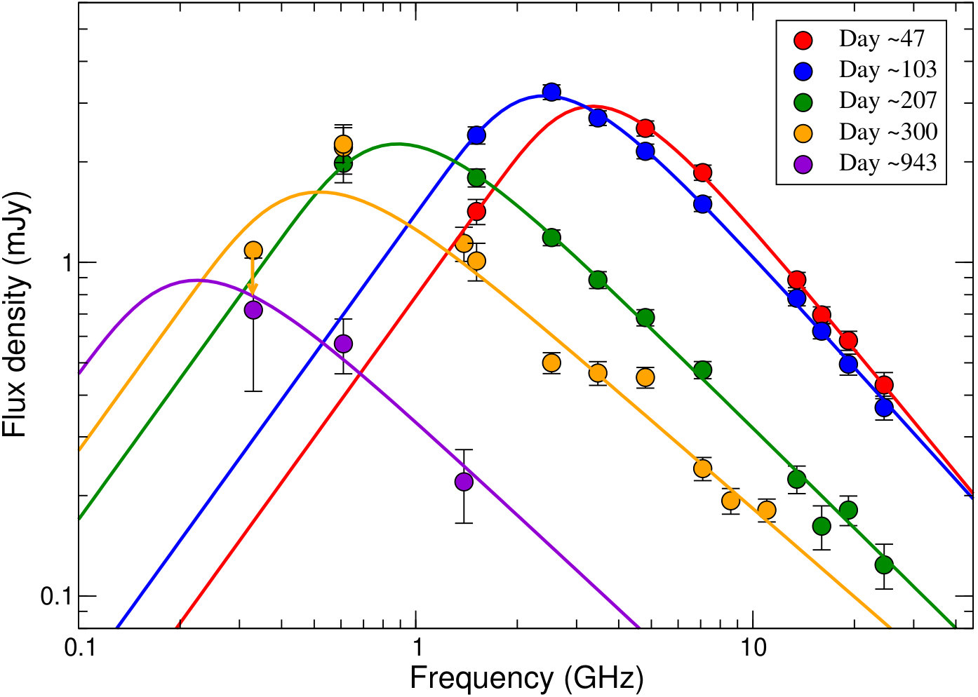 Figure 14
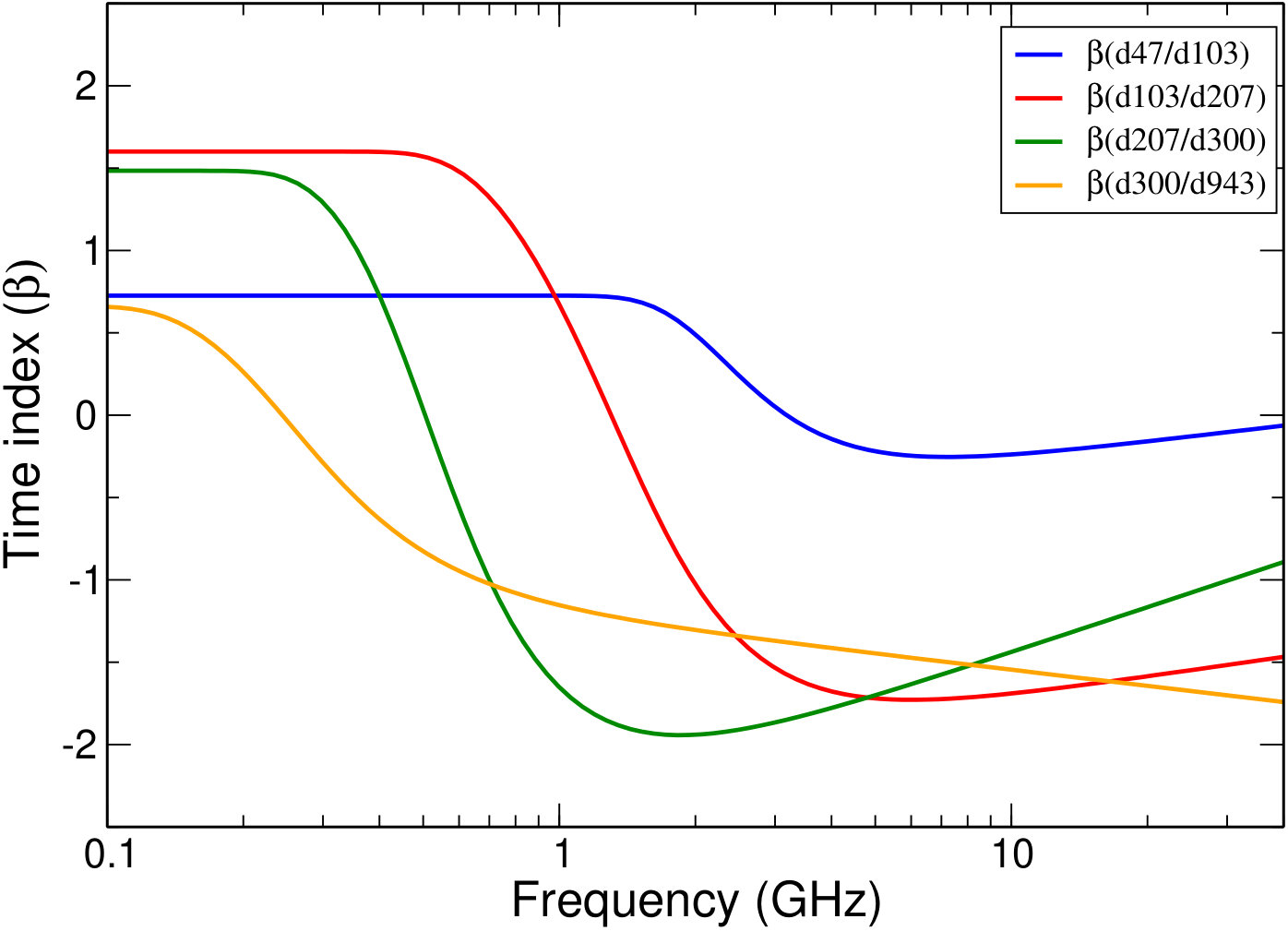 Figure 15
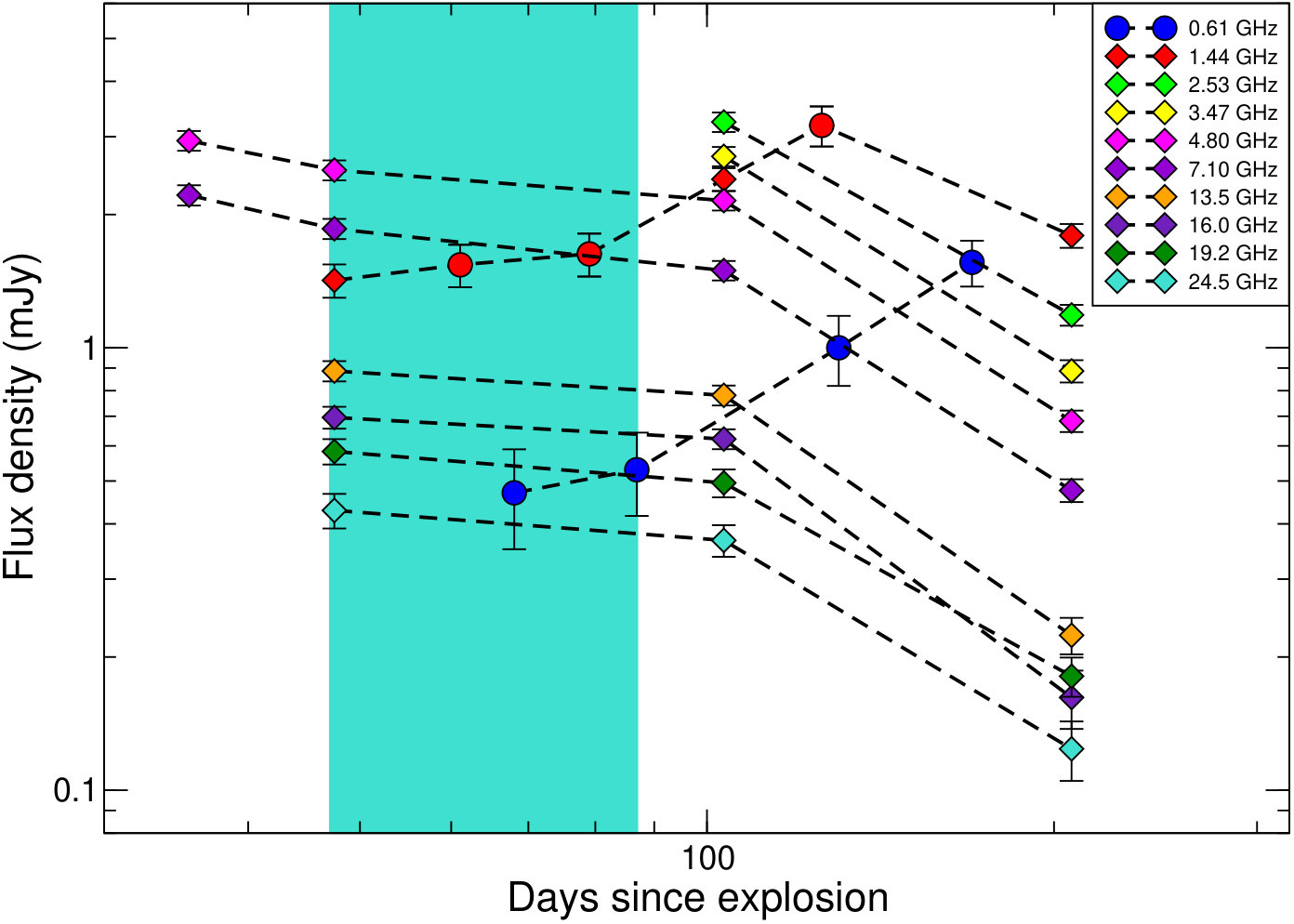 Figure 16
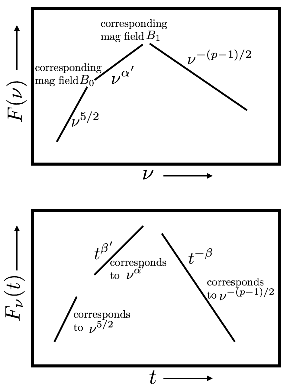 Figure 17
| Date of | AgeaaThe age is calculated assuming 2014 September 26 (UT) as the date of explosion (see §3). | Frequency | Flux density | Map rms | Resolution | |
|---|---|---|---|---|---|---|
| observation | SN | Test sourcebbNearby constant flux density test source at a position of = 12h04m29.01s, = +27∘03′45.3′′ (see §2.1.1). | ||||
| (UT) | (day) | (GHz) | (mJy) | (mJy) | (Jy beam-1) | () |
| 2014 Nov 26.1 | 61.1 | 1.39 | 1.540.17 | 6.99 0.70 | 41 | 2.30 1.95 |
| 2014 Dec 14.0 | 79.0 | 1.39 | 1.630.18 | 6.40 0.65 | 44 | 2.28 1.96 |
| 2015 Jan 29.8 | 125.8 | 1.39 | 3.180.33 | 5.85 0.59 | 50 | 3.88 2.03 |
| 2015 May 30.4 | 246.4 | 1.39 | 1.650.19 | 6.09 0.62 | 62 | 3.65 2.73 |
| 2015 Jul 04.4 | 281.4 | 1.39 | 1.330.17 | 6.37 0.64 | 46 | 2.24 1.84 |
| 2015 Jul 17.5 | 294.5 | 1.39 | 1.140.13 | 6.28 0.63 | 40 | 2.20 2.01 |
| 2015 Aug 17.5 | 325.5 | 1.39 | 0.900.11 | 5.85 0.59 | 44 | 2.59 2.06 |
| 2015 Aug 21.6 | 326.6 | 1.39 | 1.010.15 | 5.64 0.58 | 60 | 3.88 2.02 |
| 2015 Sep 18.5 | 357.5 | 1.39 | 0.850.17 | 6.96 0.72 | 80 | 8.58 3.06 |
| 2017 Apr 21.6 | 938.6 | 1.39 | 0.22 0.06 | 5.31 0.54 | 40 | 3.88 2.02 |
| 2014 Dec 03.0 | 68.0 | 0.61 | 0.47 0.12 | 13.14 1.32 | 68 | 5.14 4.18 |
| 2014 Dec 21.9 | 86.9 | 0.61 | 0.53 0.11 | 15.91 1.60 | 60 | 6.60 4.30 |
| 2015 Feb 03.1 | 130.1 | 0.61 | 1.000.18 | 15.78 1.58 | 59 | 9.03 4.74 |
| 2015 Mar 14.8 | 169.8 | 0.61 | 1.560.19 | 15.29 1.53 | 55 | 5.00 4.22 |
| 2015 May 01.6 | 217.6 | 0.61 | 1.980.25 | 16.37 1.65 | 78 | 5.76 4.30 |
| 2015 Jun 06.4 | 253.4 | 0.61 | 2.480.28 | 17.38 1.74 | 76 | 6.34 4.60 |
| 2015 Jul 10.7 | 287.7 | 0.61 | 2.210.37 | 13.86 1.40 | 98 | 4.48 3.76 |
| 2015 Jul 26.8 | 303.8 | 0.61 | 2.260.27 | 15.75 1.58 | 84 | 5.50 4.45 |
| 2015 Sep 25.3 | 364.3 | 0.61 | 1.920.23 | 15.94 1.60 | 67 | 6.20 4.70 |
| 2017 Apr 29.6 | 946.6 | 0.61 | 0.57 0.11 | 16.41 1.64 | 64 | 6.91 4.43 |
| 2015 Jul 13.5 | 290.5 | 0.33 | 362 | 9.33 8.91 | ||
| 2015 Sep 21.3 | 360.3 | 0.33 | 1290 | 11.17 7.65 | ||
| 2016 Oct 21.0 | 756.0 | 0.33 | 245 | 16.42 8.47 | ||
| 2017 Apr 27.5 | 944.5 | 0.33 | 263 | 12.03 8.17 | ||
| 2017 Nov 27.0 | 1158.0 | 0.33 | 248 | 11.58 8.00 | ||
| Date of | AgeaaThe age is calculated using 2014 September 26 (UT) as the date of explosion. | Frequency | VLA Array | Flux density | rms |
|---|---|---|---|---|---|
| Observation (UT) | (day) | (GHz) | Configuration | mJy | Jy beam-1 |
| 2014 Oct 31.5 | 35.5 | 4.799 | C | 2.9380.151 | 10 |
| - | - | 7.099 | C | 2.2130.117 | 9 |
| 2014 Nov 12.5 | 47.5 | 1.515 | C | 1.4200.123 | 80 |
| - | - | 4.799 | C | 2.5200.131 | 13 |
| - | - | 7.099 | C | 1.8580.097 | 12 |
| - | - | 13.499 | C | 0.8860.046 | 14 |
| - | - | 15.999 | C | 0.6960.040 | 18 |
| - | - | 19.199 | C | 0.5830.038 | 22 |
| - | - | 24.499 | C | 0.4290.039 | 27 |
| 2015 Jan 08.4 | 103.4 | 1.515 | CnB | 2.4040.142 | 32 |
| - | - | 2.529 | CnB | 3.2380.165 | 30 |
| - | - | 3.469 | CnB | 2.7070.137 | 15 |
| - | - | 4.799 | CnB | 2.1510.109 | 19 |
| - | - | 7.099 | CnB | 1.4950.076 | 22 |
| - | - | 13.499 | CnB | 0.7810.041 | 22 |
| - | - | 15.999 | CnB | 0.6220.032 | 12 |
| - | - | 19.199 | CnB | 0.4950.036 | 16 |
| - | - | 24.499 | CnB | 0.3670.030 | 18 |
| 2015 Apr 22.1 | 207.1 | 1.515 | B | 1.7930.111 | 14 |
| - | - | 2.529 | B | 1.1860.064 | 14 |
| - | - | 3.469 | B | 0.8860.051 | 13 |
| - | - | 4.799 | B | 0.6830.038 | 14 |
| - | - | 7.099 | B | 0.4760.028 | 13 |
| - | - | 13.499 | B | 0.2240.021 | 13 |
| - | - | 15.999 | B | 0.1620.024 | 13 |
| - | - | 19.199 | B | 0.1810.018 | 17 |
| - | - | 24.499 | B | 0.1240.019 | 21 |
| 2015 July 31.1 | 307.1 | 1.515 | A | 1.0100.130 | 17 |
| - | - | 2.529 | A | 0.5000.036 | 16 |
| - | - | 3.469 | A | 0.4660.038 | 16 |
| - | - | 4.799 | A | 0.4520.032 | 13 |
| - | - | 7.099 | A | 0.2410.019 | 12 |
| - | - | 8.599 | A | 0.1930.017 | 13 |
| - | - | 10.999 | A | 0.1810.014 | 16 |
| Date of | AgeaaThe age is calculated using 2014 September 26 (UT) as the date of explosion. | Telescope | ObsID | exposure | Count ratebbThe values are in the energy range 0.3–10 keV. | FluxbbThe values are in the energy range 0.3–10 keV. | LuminositybbThe values are in the energy range 0.3–10 keV. |
|---|---|---|---|---|---|---|---|
| obsn (UT) | day | (ks) | (counts s-1) | (erg s-1 cm-2) | (erg -1) | ||
| 2014 Oct 29.50 | 33.50 | Swift-XRT | 00033511001 | 1.98 | |||
| 2014 Nov 02.83 | 36.83 | Swift-XRT | 00033511002 | 1.61 | |||
| 2014 Nov 04.30 | 38.30 | Swift-XRT | 00033511003 | 1.61 | |||
| 2014 Nov 16.88 | 50.88 | Chandra-ACIS | 16006 | 9.65 | |||
| 2015 Nov 25.74 | 424.74 | Swift-XRT | 00084388001 | 4.59 | |||
| 2017 Jan 21.83 | 847.83 | Swift-XRT | 00033511001 | 1.65 | |||
| 2017 Oct 29.69 | 1128.69 | Swift-XRT | 00084388002 | 0.55 |
| FFA | SSA | SSA | SSA-inhomo | SSA-inhomo |
|---|---|---|---|---|
| (full data) | (full data) | (610 MHz) | (full data) | ( d) |
| d.o.f.=52 | d.o.f.=52 | d.o.f.=6 | d.o.f.=52 | d.o.f.=39 |
| AgeaaThe age is calculated assuming 2014 September 26 (UT) as the date of explosion. The range in the epochs reflect the time span of the near-simultaneous measurements. | Spectral index | Spectral index |
|---|---|---|
| Days | ||
| bbWith VLA 1.5 GHz measurement, | ||
| 0.29 | ||
Peer Reviews
No public reviews on file for this paper yet. If you reviewed it on a platform where reviews are public (OpenReview, ICLR, NeurIPS, ICML), you can paste yours below so the community can read it here.
Videos
No videos yet. Explain this paper in a talk, walkthrough, or lecture? Add one.
Type Ib supernova Master OT J120451.50+265946.6: radio emitting shock with inhomogeneities crossing through a dense shell
National Centre for Radio Astrophysics, Tata Institute of Fundamental Research, PO Box 3, Pune, 411007, India
Department of Astronomy, Stockholm University, AlbaNova, SE-106 91 Stockholm, Sweden
Nayana A. J
National Centre for Radio Astrophysics, Tata Institute of Fundamental Research, PO Box 3, Pune, 411007, India
C.-I. Björnsson
Department of Astronomy, Stockholm University, AlbaNova, SE-106 91 Stockholm, Sweden
Francesco Taddia
Department of Astronomy, Stockholm University, AlbaNova, SE-106 91 Stockholm, Sweden
Peter Lundqvist
Department of Astronomy, Stockholm University, AlbaNova, SE-106 91 Stockholm, Sweden
Alak K. ray
Homi Bhabha Centre for Science Education, Tata Institute of Fundamental Research, Mankhurd, Mumbai, 400088 India
Benjamin J. Shappee
Institute for Astronomy, University of Hawai’i, 2680 Woodlawn Drive, Honolulu, HI 96822, USA
(Received Received date; Revised Revised date)
Abstract
We present radio observations of a Type Ib supernova (SN) Master OT J120451.50+265946.6. Our low frequency Giant Metrewave Radio Telescope (GMRT) data taken when the SN was in the optically thick phase for observed frequencies reveal inhomogeneities in the structure of the radio emitting region. The high frequency Karl G. Jansky Very Large Array data indicate that the shock is crossing through a dense shell between 47 to days. The data days onwards are reasonably well fit with the inhomogeneous synchrotron-self absorption model. Our model predicts that the inhomogeneities should smooth out at late times. Low frequency GMRT observations at late epochs will test this prediction. Our findings suggest the importance of obtaining well-sampled wide band radio data in order to understand the intricate nature of the radio emission from young supernovae.
Supernovae: general — supernovae: individual Master OT J120451.50+265946.6 — radiation mechanisms: non-thermal — circumstellar matter — radio continuum: general
††journal: ApJ††facilities: Giant Metrewave Radio Telescope, Karl J. Jansky Very Large Array, Chandra X-ray Telescope, Swift X-ray Telescope
1 Introduction
Core-collapse supernovae (SNe) are energetic explosions that mark the death of massive stars with masses M 8M*⊙*. Type Ib and Ic SNe (SNe Ib/c) are characterised by absence of H and/or He lines in their optical spectra, suggesting that the outer H/He envelopes of the progenitor star were ejected before the explosion in these SNe (Woosley et al., 2002). These are collectively called stripped envelope SNe (Clocchiatti & Wheeler, 1997). Among all local SNe (distance Mpc), 19% belong to the class of SNe Ib/c (Li et al., 2011).
The proposed plausible progenitors of SNe Ib/c are Wolf-Rayet (W-R) stars that strip most of their outer envelope/s via strong stellar winds, and stars in close binary systems where H/He envelopes of the progenitor star are stripped via binary interactions (Ensman & Woosley, 1988). The physical mechanisms by which the progenitors of SNe Ib/c lose their H/He envelopes before the explosion and the time scales involved in this process remain open questions.
The progenitor systems of SNe Ib/c are poorly constrained from direct detection efforts from pre-explosion images (Smartt, 2009). However, independent constraints on the properties of SN progenitors can be obtained by studying the interaction of SNe with their circumstellar medium (CSM), formed due to mass lost from the progenitor systems during their evolutionary phases. The mass-loss during the evolution can be constant creating steady stellar winds, or can occur via episodic events (Dopita et al., 1984) creating a complex density field around the star. Radio emission, emitted via the synchrotron mechanism, is one of the best signatures to study the SN ejecta interaction with the CSM, and probes the properties of the CSM (Chevalier, 1982a).
In this work, we report the radio observations of SN Master OT J120451.50+265946.6 (hereafter SN J1204). SN J1204 was discovered on on 2014 October 28.87 (UT) by Gress et al. (2014) with an optical magnitude and at a position = 12h04m51.5s, = +26*∘59′46.6′′. The SN exploded in a galaxy NGC 4080 at a distance 15 Mpc (Karachentsev & Kaisina, 2013). SN J1204 was classified as a type Ib SN based on the spectrum obtained with the 2m Himalayan Chandra Telescope (HCT) of the Indian Astronomical Observatory on 2014 Oct 29.0 UT (Srivastav et al., 2014). Later Terreran et al. (2014) confirmed the classification using the spectrum obtained with the Asiago 1.82 m Telescope. The expansion velocity was found to be 8300 km s-1* from HeII absorption feature in the HCT spectrum (Srivastav et al., 2014). SN J1204 observations with the X-ray telescope (XRT) on-board Swift during 2014 October 29–November 04 yielded upper limits Margutti et al. (2014).
The radio emission from SN J1204 was first detected at 5 GHz with the Karl G. Jansky Very Large Array (VLA) on 2014 October 31.5 with a flux density of 3.00 0.02 mJy (Kamble et al., 2014). The Giant Metrewave Radio Telescope (GMRT) detected the radio emission at the SN position at 1390 MHz with a flux density of 1.56 mJy on 2014 November 26.09 UT (Chandra et al., 2014). In this paper, we present the results of an extensive radio follow up of SN J1204 with the GMRT, combined with the publicly available data with the VLA. Thus covering a frequency range of 0.33 to 24 GHz for more than 1000 days since discovery, we carry out detailed spectral and temporal modeling of the SN and derive the nature of the radio emission.
The paper is organised as follows: In §2, we summarise the observations at various wavebands and procedures for data analysis. We use the optical photometry data to best constrain the epoch of explosion in §3. In §4, we attempt to fit the data with the standard models of radio emission and show that this model is incapable of fitting the data. We develop and fit an inhomogeneous model to the radio data in §5. In addition, in this section, we also discuss the presence of a dense shell. Finally we discuss our results, compare the properties of SN J1204 with other stripped-envelope SNe and summarise our main conclusions in §6.
2 Observations and Data analysis
2.1 Radio Observations
SN J1204 has been extensively observed in the radio bands using the GMRT and the VLA. Below we describe the observations and procedures for data analysis.
2.1.1 GMRT Observations
\startlongtable
We started the GMRT observations of SN J1204 starting 2014 November 26.09 UT and continued monitoring observations for about 3 years. The observations covered the frequency bands of 1390, 610 and 325 MHz. The observations were carried out in total intensity mode (Stokes I), and the data were acquired with an integration time of 16.1 sec. The observed bandwidth was 33 MHz, split into 256 channels at all observed frequencies and epochs. A flux calibrator (either 3C286 or 3C147) was observed once during each observing run to calibrate the amplitude gains of individual antennas. Phase calibrators (J1125+261, J1227+365 or J1156+314) were observed every minutes for minutes throughout each observing run to correct for phase variations due to atmospheric fluctuations. The data were analysed using the Astronomical Image Processing System (AIPS). Initial flagging and calibration were done using the software FLAGCAL, developed for automatic flagging and calibration for the GMRT data (Prasad & Chengalur, 2012). The flagged and calibrated data were closely inspected, and further flagging and calibration were done manually until the data quality looked satisfactory. The calibration solutions obtained for a single channel were applied to the full bandwidth. Instead of averaging the full bandwidth, only a few channels (20 channels for 1390 MHz band, 15 channels for 610 MHz band and 7 channels for 325 MHz band) were averaged together to avoid bandwidth smearing. Fully calibrated data of the target source was imaged using the AIPS task IMAGR. A few rounds of phase self calibration and one round of amplitude plus phase (a&p) self calibration were performed. During the a&p self-calibration, the voltage gains were normalized to unity to minimize the drifting of the flux-density scale. In addition, the flux densities of SN J1204 and the test source were measured between the a&p and the last phase self-calibration rounds and they were found to be consistent. The flux density of the SN was measured by fitting a Gaussian at the SN position using the AIPS task JMFIT. This is a standard procedure followed for the GMRT data analysis (e.g. Chandra & Kanekar, 2017, and references therein). The data on 2015 April 25 were found to be corrupted and we did not use it for further analysis. The details of GMRT observations and the SN flux densities are summarised in Table 1.
To estimate whether there is a contribution from the host galaxy at the SN position, in Fig. 1 we plot the the contour map for the SN field. We do not find any contamination by the host galaxy at the SN position within 3 noise.
To confirm if the variability seen in the SN flux density at various epochs is real, we chose a nearby non-variable test source NVSS J120428+270343 at a position of = 12h04m29.01s, = +27*∘03′45.3′′*. The source was selected such that its flux density was found to be constant within the uncertainties of 10% of the source flux between the NVSS (Condon et al., 1998) and the FIRST (White et al., 1997; Helfand et al., 2015) surveys. The flux density of the test source in our observations is constant within % errors at 1390 and 610 MHz bands and within % at 325 MHz band at various epochs (Table 1). This is roughly consistent with the uncertainties in the GMRT data due to systematic errors (Chandra & Kanekar, 2017). Thus for fitting the data, we add 10% uncertainty in quadrature at 1390 and 610 MHz bands and 15% at 325 MHz bands.
2.1.2 VLA Observations
We analysed the publicly available archival VLA data for SN J1204 at five epochs from 2014 October 31 to 2015 July 31 spanning a frequency range of 1–24 GHz. The data had bandwidth of 1 GHz split into 8 spectral windows at 1.515 GHz, and 2 GHz split into 16 spectral windows for all other frequencies. We carried out the VLA data analysis using standard packages within the Common Astronomy Software Applications package (CASA, McMullin et al., 2007). CASA task ‘clean’ was used to make images of the data. The details of the VLA observations, array configurations and the flux densities of the SN are summarised in Table 2. We add 5% error in the quadrature for the VLA data, a typical uncertainty in the flux density calibration scale at the observed frequencies 111https://science.nrao.edu/facilities/vla/docs/manuals/oss/performance/fdscale.
2.2 Optical Observations
We used the data from All-Sky Automated Survey for Supernovae (ASAS-SN, Shappee et al., 2014) in V-magnitude band, covering pre-explosion phase up to 400 days before the assumed explosion date until 1200 days post-explosion. ASAS-SN images were processed by a fully automatic ASAS-SN pipeline using the Interactive Spectral Interpretation System (ISIS; Houck & Denicola, 2000) image subtraction package (Alard & Lupton, 1998; Alard, 2000). For this the stacking was done on the three dithered images before carrying out the photometry. For the subtraction, the stacked images were subtracted from a good reference image. We performed aperture photometry on the subtracted images using Image Reduction and Analysis Facility (IRAF; Tody, 1986, 1993) ‘apphot’ package and calibrated the results using the AAVSO photometric All-sky Survey (APASS; Henden et al., 2015). Some of the data points were found to be affected by clouds in the FOV or by the incidence of cosmic rays; and these data were discarded. The ASAS-SN detections and 3 limits are shown in Fig. 2. SN J1204 is, unfortunately, only detected after a seasonal gap which resulted in missing the peak of the SN light curve.
2.3 X-ray Observations
SN J1204 was observed with the Swift-XRT covering a period almost up to 1000 days since its discovery. In addition, Chandra observed it for around 10 ks on 2014 Nov 16. We analysed the publicly available archival data from both the telescopes (see Table 3).
For the Chandra data analysis, the Chandra Interactive Analysis of Observations software (CIAO; Fruscione et al., 2006) was used. We extracted spectra, response and ancillary matrices using the CIAO task specextractor. The CIAO version 4.9 along with CALDB version 4.7.6 was used for this purpose.
The Swift-XRT spectra and response matrices were extracted using the online XRT products building pipeline222http://www.swift.ac.uk/user_objects/ (Evans et al., 2009; Goad et al., 2007). We used the XRT specific tasks XSELECT, XIMAGE and SOSTA of the package HEAsoft333http://heasarc.gsfc.nasa.gov/docs/software/lheasoft/ to carry out the spectral analysis and obtained 3- limits on the count rates.
The SN was not detected in any of the X-ray observations. The count-rate simulator WebPIMMS 444https://heasarc.gsfc.nasa.gov/cgi-bin/Tools/w3pimms/w3pimms.pl, using a temperature of 5 keV and Galactic absorption column density of cm*-2* towards the SN direction (Dickey & Lockman, 1990; Kalberla et al., 2005), was used to estimate the upper limits on the unabsorbed flux of the SN in Table 3. A distance of 15 Mpc was used to convert the fluxes into unabsorbed luminosities.
3 Constraining the explosion epoch
There is a large uncertainty in the date of explosion for SN J1204. The HCT spectrum on 2014 Oct 29.0 UT best matched with several normal type-Ib SNe a few weeks after the maximum (Srivastav et al., 2014). Since the typical rest-frame rise time of Type Ib SNe is days (Taddia et al., 2015), the explosion date is likely to be 30–50 days before the discovery.
We attempt to estimate the explosion epoch based on the optical light curves. Our data are mainly in the -band from the ASAS-SN observations, but we also have an unfiltered magnitude point from the discovery telegram (13.9 mag at JD 2456959.37; Gress et al., 2014) obtained by the MASTER Global Robotic Net (Lipunov et al., 2010). The discovery magnitude was significantly brighter than the rest of the data, suggesting that the SN was discovered around the peak and that the rest of the data belong to the linear tail of the light curve. To quantify the phase of our observations with respect to the -band peak magnitude, we compared them to the stripped-envelope SN light curve templates from Taddia et al. (2018), in the - as well as in the - bands. The match between our data and the templates is shown in Fig. 3. Here we considered that on average stripped-envelope SNe peak 0.124 mag brighter in the -band than in the -band, and that the peak in the -band occurs 1.23 days after the one in the -band (Taddia et al., 2018). We also assumed that the open-filter magnitude from MASTER can be treated as a -band point (see e.g., Tsvetkov et al., 2017). Finally, we only considered the first four - band points for the fit, which are those within 50 days since maximum, when the -band template has a relatively small spread. From the best match between the data and the templates we derive the -band peak epoch (JD 2456946.553.00). From this epoch we subtracted the average -band rise-time for SNe Ib (from Taddia et al., 2015), which is 20.071.86 d. This gives the best explosion date to be JD 2456926.53.5. This corresponds to UT date of 2014 September 26 within an uncertainty of 3.5 days. This error on the explosion epoch takes into account the typical light curve shape of stripped envelope SNe. In the unlikely case that SN J1204 is similar to SN 2005bf or 2011bm, i.e., to rare stripped envelope SNe with long rise times, then our explosion epoch would have happened between 10 and 20 days earlier.
We note that for the computed -band peak epoch, the classification spectrum (obtained on October 29th 2014, Srivastav et al., 2014) occurred 13 days after the peak, consistent with the phase indicated by them (a few weeks after maximum). Furthermore, the Helium-I velocity of 8300 km s*-1* reported by Srivastav et al. (2014) is in line with the average Helium-I velocities measured for SNe Ib at that phase after peak (Taddia et al., 2018). Thus in this paper, we assume 2014 September 26 UT as the date of explosion for SN J1204.
4 Modeling and results
4.1 Visual inspection of the data
SN J1204 is one of the handful SNe for which extensive data exist at radio frequencies. In Fig. 4(A), we plot all the radio data from 0.33 GHz to 24.5 GHz frequency bands covering the epochs 35 days till 1158 days. In addition, we plot near-simultaneous spectral indices at various adjacent frequencies and various epochs in Fig. 4(B).
The first look at the data reveal that the data are optically thin at frequencies higher than 2.53 GHz onwards. A significant fraction of low-frequency ( GHz) data are in optically thick phase. The first two observations at 0.33 GHz resulted in upper limits prohibiting us from constraining the absorption peak at this band, however, we are able to constrain it at other two GMRT frequencies. The 1.39 and 0.61 GHz light curves peak on d (peak flux density mJy) and d (peak flux density mJy), respectively. The peak spectral luminosity at 1.39 GHz is erg s*-1* Hz*-1*, consistent with the radio spectral luminosity of SNe Ib/c which spans a range of erg s*-1* Hz*-1* (Soderberg, 2007).
4.2 Standard model of radio emission
In a SN explosion, stellar ejecta are thrown out into the CSM at supersonic velocities, which drive a ‘forward’ shock propagating into the CSM and a ‘reverse’ shock moving back into the ejecta. Electrons are accelerated to relativistic energies in the forward shock via diffusive shock acceleration and produce synchrotron radiation in the presence of amplified magnetic fields. A model for the ejecta-CSM interaction and its evolution was developed by Chevalier (1982b). This model follows self-similar solution with the shock radius evolving as power-law in time, i.e. , where is the shock deceleration parameter which is connected to the outer ejecta density profile (in ) as . Here is index of the unshocked CSM density profile, , created by the stellar wind of the progenitor star (). For a steady stellar wind, .
The radio emission in SNe can be initially suppressed either due to free-free absorption (FFA) by the ionised CSM (Chevalier, 1982b) or/and due to synchrotron self-absorption (SSA) by the same electron population responsible for the radio emission (Chevalier, 1998). These processes can be distinguished via their early radio light curves and spectra in the optically thick phase. As the shell expands, the optical depth decreases and at optical depth unity SNe spectra show transition from optically thick to optically thin regime indicated by a change in the sign of spectral index. Observations spanning over this transition are critically important to pin down the dominant absorption processes, which give information about the magnetic field, size of the emitting object, density, mass-loss rates etc.
Even though SNe Ib/c generally have SSA as the dominant absorption mechanism, we start our modeling considering both FFA and SSA mechanisms.
In a model where FFA is the dominant absorption mechanism, the radio flux density, , can be expressed as (Weiler et al., 2002)
[TABLE]
where K1 is a normalization factor whose value will be equal to the radio flux density at 1 GHz measured on day 100 after the explosion. The parameters and denote the spectral and temporal indices, respectively, in the optically thin phase. The radio spectral index can be related to the electron energy index (in ) as . Here is the optical depth characterized by the free-free absorption due to the ionized CSM external to the emitting material, and can be written as
[TABLE]
where denotes the free-free optical depth at 1 GHz measured on day 100 after the explosion. As the blast wave expands, the optical depth decreases with time as , where the index of optical depth evolution is related to shock deceleration parameter as .
For the SSA dominated synchrotron emission from SNe, the radio flux density can be written as (Chevalier, 1998):
[TABLE]
where the optical depth is characterised by SSA due to the relativistic electrons at the forward shock. The SSA optical depth is given by
[TABLE]
K1 and K2 are the flux density and optical depth normalisation factors similar to the case of FFA. The flux density in the optically thick and thin phases evolve as and , respectively. Here spectral index is related to electron energy index as . Similar to FFA model, is the time evolution of flux density in the optically thin phase, whereas, is the flux density evolution with time in the optically thick phase. While depends on shock deceleration parameter , depends on as well as electron energy index . The exact form depends upon the scalings of magnetic field, , and the electron energy density (Chevalier, 1996). For example, if magnetic energy density and relativistic electron energy density scale with post shock energy density (model 1 of Chevalier, 1996), then optically thick light curve will lead to and then . This involves an assumption that the magnetic field was built up by turbulent motions. However, if compression of the CSM magnetic field determines the relevant magnetic field scaling and relativistic electron energy density scales with the flux of particles into the shock front, then and (model 4 of Chevalier, 1996). When there are substantial data in the optically thick phase, the parameters , and can be independently obtained, and one can determine the relevant scalings in a particular case.
We now model the full data using both the FFA and the SSA models. We first perform the FFA model fit keeping , , , and as free parameters. The best-fit parameters are obtained using the minimisation. The fitted models along with the measured spectra and light curves are shown in Figs. 5 and 6. The best-fit parameters are given in the Table 4. We note that the reduced chi-square () for the FFA model is quite high (), suggesting that the FFA model is not a good fit to the radio data.
We now fit the data with the SSA model as given in Eqns. 3 and 4. The best-fit parameters for the SSA model are given in Table 4 and plotted in Figs 5 and 6. The reduced chi-square is this case is . While the SSA model performs slightly better than the FFA model, it fails to provide an acceptable fit to the data.
5 A need for a non-standard model
Unfortunately neither the FFA nor the SSA models provide a good fit to the radio data of SN J 1204. Visual inspection of Figs. 5 and 6 suggests that the data days are not fit well with the standard models. The model over-predict the flux on d and under-predict the flux at d. The low frequency light curves show flattening at the early epochs in the optically thick phase. The discrepancies between data and models are more pronounced at earlier epochs.
To understand the early time behaviour of the radio data, we investigate the estimated spectral indices in the optically thick phase, which are mainly at the GMRT frequencies. We plot them in Fig. 7 and tabulate in Table 5. We notice that during the first three epochs, i.e. between days 64 to 127, the spectral indices are . This value is much flatter than the spectral index 2.5 expected in the SSA model or steeper value in the FFA model. The values of is a lower limit on day 289, which is also consistent with the above values.
While the spectral indices are expected to flatten near the spectral peaks, the 1390 MHz peak occurs at day 126 and 610 MHz peak much later (see §4.1). Thus only the last data point around 127 d may be affected by this effect. The fact that the spectral indices have flatter values from 64 d onwards, indicates that this is a real effect. The average value of the optically thick spectral index from the first three epochs is (Fig. 7).
To probe the nature of absorption further, we look at the radio light curve at 610 MHz, the best sampled frequency in the optically thick phase. We again fit the standard FFA and SSA models, using Eqns. 5 and 6, respectively.
[TABLE]
[TABLE]
While the FFA model gives a poor fit, SSA model seems to fit the data reasonably well (Fig. 8). However, the best fit values of and obtained in these fits (column 3 of Table 4) will imply and . The value of is unrealistically small and is inconsistent with the observations (Fig. 4). The derived value of is much smaller than typical values seen in Type Ib SNe and will indicate very high deceleration at this young age, which is unlikely. Hence we conclude that despite providing acceptable fit, the standard SSA model does not represent a physically viable model to 610 MHz light curve.
Unphysical values of model parameters obtained above combined with the much flatter spectral index in the optically thin phase, , indicate that the standard homogeneous SSA emission model does not fit the radio emission in SN J1204.
5.1 An inhomogeneous model
Björnsson (2013) and Björnsson & Keshavarzi (2017) have explained the flatter optically thick evolution of the radio spectra in terms of inhomogeneities in the radio emitting region caused by the variations in the distribution of magnetic fields and relativistic electrons. Björnsson & Keshavarzi (2017) have shown that if the emission structure is inhomogeneous, then fitting a standard homogeneous model to observations around the peak frequency gives a lower limit to the source radius. Björnsson (2013) and Björnsson & Keshavarzi (2017) have quantified the variation of the magnetic field over the projected source surface by a source covering factor, . As per their formulation, even though the locally emitted spectrum is that of standard synchrotron, the will give rise to a range of optical depths over the source, broadening the observed spectrum. Since the covering factor is maximum at frequencies substantially below that of the spectral peak (Björnsson & Keshavarzi, 2017), the detailed observations at low frequencies are best to probe the inhomogeneities.
In §A, we develop an inhomogeneous emission model adopted from Björnsson & Keshavarzi (2017). As per this formulation, the inhomogeneous model will alter the spectra for magnetic fields ranging between (Fig. A.1), and radio emission will follow the standard homogeneous SSA formulation at frequencies corresponding to magnetic fields outside this range, i.e.
[TABLE]
Here is the SSA frequency, is defined as , where is the probability of finding a particular value of within and (Eq. A1). We define as spectral index in the SSA optically thick phase in the inhomogeneous model. Thus in our case . Here indicates a correlation between the distribution of relativistic electrons with the distribution of magnetic field strengths (see §A). For the inhomogeneities in the relativistic electrons distribution are not correlated with the inhomogeneities in the magnetic field. For , the inhomogeneities between the two distributions are correlated.
Since our radio observations in the optically thick phase indicate at all epochs, this suggests we are in the regime for observed frequency range. For the observed in the optically thick phase, and for , we obtain for and for .
In order to take the inhomogeneities into account, we use a model, in which optically thick spectral index follows in Eqns. 3 and 4 :
[TABLE]
where the optical depth is characterised by the SSA due to the relativistic electrons at the forward shock. The SSA optical depth is given by
[TABLE]
The best fit values are tabulated in column 4 of Table 4. We plot the best fit inhomogeneous model in Figs. 5 and 6. While the inhomogeneous model fits are better than the standard SSA and FFA fits, and improved by nearly a factor of , the early data still deviates from the inhomogeneous SSA model. Fig. 6 indicates that the model spectrum on day does not represent the data well.The model light curves at early epochs are also discrepant with the data (Fig 5 ).
This suggests that a global model assuming constant , and will not fit the data well at all the epochs. This situation can be reconciled if there is an evolution in the blast-wave parameters with time, likely at early epochs.
5.2 Shock passing through a shell
To understand the dynamical evolution of the blast wave and to investigate the inconsistency with the global fit parameters, we study the near-simultaneous spectra of the SN at individual epochs (Fig. 9.) Since we established the need for an inhomogeneous model in §5.1, we model the spectra of SN J1204 at each epoch with the inhomogeneous SSA model:
[TABLE]
where we use . is the peak flux density at a frequency at a given epoch.
There are a few things to decipher from the individual spectra. The spectra evolve very little between days and (Fig. 9). The peak flux density and peak frequency have a nearly flat evolution and between these two epochs. In addition, we note that there are 7 and 8 independent data points in spectra on day 47 and 103, respectively, and all of these data are consistent with much slower evolution than expected in the standard synchrotron emission model. This can also be seen in the time evolution plot, where is close to zero at high frequencies during these two epochs. Such a situation may arise if the shock is crossing through a shell and has slowed down due to a high density of the shell, causing the time evolution of the parameters to slow down between these two epochs.
While it is difficult to decipher the exact duration for which the shock is passing though the shell, we attempt to constrain it based on our radio data. For this purpose, we re-plot the light curve zooming into early times (Fig. 10). Fig. 10 indicates that while the flux density in the earliest data between day 35 and 47 evolves as and at 4.8 and 7.1 GHz bands, respectively, the evolution of the flux density slows down as and between days 47 to 103, respectively. This again steepens and evolves as and post day 110. While the relatively flatter evolution between 35 and 47 days at 4.8 and 7.1 GHz bands could be reconciled with a situation where we may be witnessing the shock soon after the peak transition at these frequencies and tracing the broader top likely due to inhomogeneities, the significant flattening between day 47 and 103 cannot be explained in this framework.
This suggests that shock was probably moving into a smooth CSM at the first epoch , but entered into a higher density shell some time during . The steep evolution between days 103 and 207 suggests that it was out of the shell by the time VLA observations commenced on . An additional clue on the length of time it took for the shock to cross the shell comes from the optically thick data points at 1.4 and 0.6 GHz bands. The first three epochs of 1.4 GHz light curves (covering days), and first two epochs at 0.61 GHz (covering days) are flatter than the other optically thick data points at this frequency (Fig. 10). This indicates that shock likely stayed in the dense shell up to d and was out of the shell afterwards. Thus we infer that the shock likely remained in the shell during to days after the SN explosion. However, we note that the transition at day is much less secure than that at day .
After emerging from the shell, the shock velocity is expected to stay roughly constant (van Marle et al., 2010) or even accelerate (Harris et al., 2016). This transition phase may last a few dynamical timescales, i.e., until the swept-up mass starts to dominate the extra mass in the shell. Regardless of the details of this phase, the time evolution of should speed up and approach that pertaining to the time before the shock entered the shell.
In order to evaluate the possible effects of FFA after the shock entered the shell, we examine , which is the FFA optical depth at . As discussed by Björnsson & Lundqvist (2014), this is a maximum value for the free-free optical depth , because it is set by the temperature resulting from the actual heating due to the absorbed synchrotron emission itself. Neglecting terms of order unity, is (Björnsson & Lundqvist, 2014)
[TABLE]
where is the velocity of the forward shock in . The density of the CSM is , where is the steady mass loss rate of the progenitor star in units of solar masses per year and is the corresponding wind velocity in units of 10 km s*-1*, respectively. Since it is likely that the shock velocity is larger than km s*-1* at d, and GHz on this day (Fig. 9), Eq. 11 imples
[TABLE]
Since SN J1204 is a Type Ib SN, is expected. Unless the mass-loss rate is unusually large (i.e., ), FFA should be negligible in the wind; for example, a wind velocity of km s*-1* and give .
Although hydrodynamical simulations are needed to describe the passage of the shock through the shell, Eq. 11 can be used to estimate its FFA. Initially, when the forward shock impacts the shell, the already shocked mass between the forward and reverse shocks will act as a piston. The shock velocity in the shell is then given, roughly, by momentum conservation, i.e., the shock velocity slows down by a factor . Here, is the shell density and the density behind the forward shock at impact. Furthermore, observations show that the duration of the shell passage is roughly equal to the time for the forward shock to reach the shell. The width of the shell is then . The FFA of the shell can then be obtained by multiplying the RHS of Eq. 11 with ; for example, with and , a FFA optical depth of unity in the shell corresponds to . For a strong shock, the density in the wind is , which gives a density contrast between the shell and the wind of . Furthermore, the associated slow-down of the shock velocity would be by a factor . In the standard model, the values of and are expected to evolve roughly inversely with time (cf. also the analytical fits done above). As shown in Figs. 9 and 10, the observed slow-down is substantially less than this. Hence, the optical depth to FFA in the shell should also be substantially below unity at 3.5 GHz. and the density contrast between the shell and the wind is expected to be less than .
There is another puzzle. If the shock is passing through a dense shell, one would expect the optically thin emission to increase due to the continuous injection of relativistic electrons. But Fig. 10 clearly shows that the flux evolution at 4.8 GHz and higher frequenies is flatter and optically thin. This could have been explained by cooling, but Fig. 4(B) indicates that the optically thin spectral indices are mostly consistent with near constant values and do not show any particular steepening in this duration. Thus cooling is unlikely to be the reason for flatter optically thin light curves. Björnsson (2013) has explained this situation where a constant magnetic field is confined within a small distance from the shock front in the inhomogeneous model (their Eq. 4). In such a case, relativistic electrons are continuously entering the shocked shell and cascading downwards, hence leaving the width of the radio emitting region almost constant. Thus the main contributions to both emission and absorption come from near the shock boundary, and give rise to flat light curves seen at the VLA frequencies. This would then be consistent with a situation where the inhomogeneities are confined mainly to the magnetic field distribution, whereas, the relativistic electrons are distributed more or less uniformly (Fig. 11). If this is indeed the case, it suggests in Eq. 7.
5.3 Combining with the multiwavelength Data
The Swift-XRT data covered the epochs between days 33 and 1128 since explosion, however, the most important constraints come from the Chandra data on day 51. At such early times, inverse Compton scattering of photospheric photons can contribute significantly to the X-ray emission in Type Ib/c SNe, and this prediction can be tested.
In Fig. 12, we plot the radio, X-ray and optical luminosities for SN J1204. The X-ray luminosity is at least three orders of magnitude lower than the optical luminosity. Björnsson (2013) estimated a quantity , where , and are the X-ray, bolometric and radio luminosities, respectively, normalized to their respective values for another stripped envelope SN 2003L. They found that this quantity does not change significantly for various Type Ib/c SNe and remains close to 1, even though the individual values of , , and are very different. With the lack of X-ray detection as well as unavailability of measurement of bolometric luminosity in SN J1204, we cannot measure this parameter. However, the observations with Chandra around day 51 gives the most constraining upper limits on the X-ray luminosity and the ASAS-SN data in the V-band can be treated as a lower limit on . Using these values, we can constrain the above ratio, for SN J1204, scaled to the respective values for SN 2003L (Soderberg et al., 2006), to be . This is indeed an upper limit and the actual value could be much smaller and may fit in with the values obtained from other SNe Ib/c (Fig. 1 of Björnsson, 2013). Björnsson (2013) also found this quantity to not evolve with time significantly, suggesting that . This is consistent with a scenario in which a substantial contribution to the X-rays come from inverse Compton scattering of photospheric photons (Björnsson, 2013). Thus inverse Compton scenario implies an inhomogeneous source structure or vice-versa, if the equipartition fraction is not too far away from unity (Eq. 22 of Björnsson, 2013).
5.4 Final comprehensive model
Connecting all the pieces together as discussed in the previous sections, we establish that the radio emission from SN J1204 is arising from the shock which has inhomogeneities, and is passing through a shell during epochs to since explosion. Hence we fit the inhomogeneous SSA model excluding all the data till day 87. We again use the formalism described in Eqns. 8 and 9. The best fit model parameters are detailed in column 5 of Table 4. While the is still not a statistically very good fit, we consider it a reasonably acceptable fit. We plot the spectra at four representative days and light curve at four representative frequencies in Fig. 13. Here the shaded region in the light curves indicate the data excluded from the modeling. These figures indicate that the inhomogeneous model fits the data reasonably well. Unfortunately, it is difficult to quantitatively constrain the data before day 87.
6 Discussion and Conclusions
In this paper we have described the radio observations of SN J1204 up to around 1200 days after the explosion covering the frequency range from 0.33 GHz to 25 GHz. The radio observations of SN J1204 suggest that the radio emitting region is inhomogeneous where the magnetic field is confined within a small distance from the shock front. The data reveal that the shock is passing through a shell during to days.
The GMRT low frequency data in the optically thick phase are crucial to indicate the presence of inhomogeneities in the synchrotron emitting region, which is responsible for the flattening of the optically thick spectral index to . Flattened light curves and spectra have been seen in several SNe Ib/c, e.g., SNe 1994I (Weiler et al., 2011), 2003L (Soderberg et al., 2005) etc. Weiler et al. (2011) explained the flattened profile in SN 1994I due to free-free absorption process intrinsic to the synchrotron emitting source with the thermal electrons distributed roughly as the relativistic ones, however, this scenario within the standard synchrotron model gives discrepant results (Björnsson & Keshavarzi, 2017). While such an intrinsic FFA mechanism is possible in Type IIn SNe due to their high densities (e.g. Chandra et al., 2012), it is very unlikely in SNe Ib/c which are expected to have Wolf-Rayet (W-R) progenitors.
The ratio of for SN J1204, where , and are normalized to their respective values for SN 2003L , is . However, it is an overestimation since we use X-ray upper limit to substitute for the X-ray luminosity and ASAS-SN V-band luminosity as a proxy for bolometric luminosity. Hence our value of is not discrepant with other SNe Ib/c, indicating inverse-Compton effects likely to be important when the shock has inhomogeneities (Björnsson, 2013).
Since our radio observations cover a large span of time, we have been able to fit the individual spectra up to around days post explosion. The spectra between days 47 and 103 suggest rather insignificant time evolution in the shock parameters (Fig. 9). We have explained this in a scenario in which the shock is moving through a higher density shell between and days. We show in §5.2 that the FFA optical depth in the shell is not expected to increase by more than a factor of 2 and is likely to not alter the radio spectra significantly. Recently published optical spectroscopic data by Singh et al. (2019) indicate no obvious new features associated with the shock impacting the shell. This indicates that the emission comes mainly from the ejecta and that the contribution from the shocked material is negligible. The lack of any signs of the shell-interaction would then be consistent with a rather low shell mass, i.e., a low FFA optical depth.
A major issue here is that when the shock is crossing the shell, one would assume the optically thin flux to increase in this duration due to continuous injection of electrons. This is contrary to what VLA data reveal, i.e. flatter optically thin light curves. While this situation could have been reconciled in the presence of cooling, our data has suggested an absence of cooling. We find that the early time flatter optically thin light curve evolution during the shell-crossing phase is consistent with a scenario where the magnetic field distribution is confined within a small region of the shock, whereas, the relativistic electrons are distributed more uniformly and the width of emission region stays nearly constant (Fig. 11).
SNe Ib/c are understood to be explosions of massive stars whose hydrogen envelopes have been stripped off before the explosion (Woosley et al., 2002), but the physics of the process by which stars lose their outer envelopes, and the corresponding time scales are still debated (Smith et al., 2011). The presence of a shell during to days in SN J1204 could be a clue to the stripping of the hydrogen/helium shell of the progenitor, possibly from a binary system (Podsiadlowski et al., 1992). Evidence of this has been seen in for SNe Ib/c SN 2001em (Soderberg et al., 2004) and SN 2014C (Vinko et al., 2017), where evidence of Balmer recombination lines have been seen. In SNe 2001em and 2014C, the flux density enhancement was observed at a late time, i.e. day 677 for SN 2001em (Stockdale et al., 2005; Chugai & Chevalier, 2006) and day 400 for SN 2014C (Anderson et al., 2017). This suggested that the shells were ejected several decades before the explosion. However, in case of SN J1204 we find the evidence of dense shell just 47 days after the explosion, lasting for days. Due to lack of constraints on ejecta and wind velocity, we cannot determine the pre-explosion epoch at which shell was ejected, but it could not have been too long ago, unlike SNe 2001em and 2014C, as W-R are known to have fast winds. We have checked the archival ASAS-SN data to search for possible signatures of pre-SN ejection. The ASAS-SN V-magnitude photometric observations begin 600 days pre-SN and do not show evidence of pre-SN ejection episodes (Fig. 2), however, there is no data at many epochs. Recent campaigns to observe SNe within days of explosion have revealed narrow emission lines of high-ionization species in the earliest spectra of luminous SNe II of all subclasses. These flash ionization features indicate the presence of a high-density medium close to the progenitor star (Hosseinzadeh et al., 2017). In our case, the SN was detected after the optical maximum and hence no such data are available.
The optically thin spectral index remains close to at all epochs. This would suggest , which is steeper than expected () from the standard diffusive shock acceleration theory. In absence of cooling, this situation can be reconciled if the diffusive shock acceleration is so efficient that the whole process becomes nonlinear (Chevalier & Fransson, 2006). The prediction of such a process is a flatter profile with time, albeit evolving very slowly (Chevalier & Fransson, 2006). This can be tested at late epochs low frequency observations.
In §C, we have derived the evolution of covering factor . For SN J1204, is positive, indicating that the time evolution for is positive (Eq. C4). This means the inhomogeneities should smooth out if followed long enough. We are continuing to observe SN J1204 at GMRT frequencies, especially at 325 MHz band, and these observations will test the above hypothesis, and reveal whether the synchrotron emitting region has emerged into a homogeneous one at late epochs.
To summarise the main conclusions of this work, the radio frequency observations of SN J1204 have revealed that the radio emission is arising from a shock with inhomogeneities mainly in the magnetic field distribution behind the shock (as sketched in Fig. 11). This shock is passing through a higher density shell for during to days. Low frequency sensitive telescopes like GMRT provide excellent opportunity to carry out such low frequency studies to reveal the nature of synchrotron emitting regions. With three times increased sensitivity as well as the near continuous and low-frequency wide bands of the upgraded GMRT (Gupta et al., 2017), such studies will be possible for a large number of SNe in the future.
We thank the referee for constructive comments, which helped improve the manuscript significantly. We acknowledge substantial help from Subo Dong, Jose L. Prieto, Krzusztof Z. Stanek, Christopher Kochanek, Todd Thompson and Tom Holoien for the ASAS-SN data, and Roger A. Chevalier. P.C. acknowledges support from the Department of Science and Technology via SwaranaJayanti Fellowship award (file no.DST/SJF/PSA-01/2014-15). A.R. acknowledges Raja Ramana Fellowship of DAE, Govt of India. We thank the staff of the GMRT that made these observations possible. GMRT is run by the National Centre for Radio Astrophysics of the Tata Institute of Fundamental Research. The National Radio Astronomy Observatory is a facility of the National Science Foundation operated under cooperative agreement by Associated Universities, Inc. This research has made use of data obtained through the High Energy Astrophysics Science Archive Research Center Online Service, provided by the NASA/Goddard Space Flight Center.
Appendix A Inhomogeneous spherically symmetric model
In a homogeneous spherically symmetric model for Type Ib/c supernovae (SNe Ib/c), the radio emission is usually fit with a synchrotron emission model, suppressed at early times by synchrotron self-absorption (SSA) with a frequency dependence of the flux density as . However, inhomogeneities in an otherwise spherically symmetric emission structure can cause broadening in the observed radio spectra and/or light curves (Björnsson, 2013). SSA frequency is quite sensitive to the presence of inhomogeneities and can be used to identify these in the source structure.
The inhomogeneities can arise by variations in the relativistic electrons distribution and/or the magnetic field strength within the synchrotron source. Björnsson & Keshavarzi (2017) have derived the formalism for the inhomogeneous synchrotron source, assuming planar geometry, in terms of the covering factor characterizing the optically thick properties and the filling factor characterizing the optically thin properties of the radio emission. Here we discuss the relevant formalism taken mainly from Björnsson (2013); Björnsson & Keshavarzi (2017) in the context of this paper. Here it is assumed that the locally emitted spectrum is that of standard synchrotron model, however, the inhomogeneities in the magnetic field () will give rise to variation in optical depths and superposition of spectra with varying optical depths will broaden the resulting spectrum.
The source covering factor has been defined to describe the variation of the average magnetic field strength over the projected source surface. If is the probability of finding a particular value of within and , then the source covering factor will be parameterized from and can be written as
[TABLE]
Here we define magnetic field such that frequencies smaller than the frequency corresponding to SSA at , i.e. follow standard synchrotron model in optically thick phase, and such that frequencies larger than the frequency corresponding to SSA at , i.e. follow standard synchrotron model in the optically thin phase (Fig. A.1). Between these two boundaries, the covering factor will modify the spectral flux as
[TABLE]
The frequency dependence follows (Björnsson & Keshavarzi, 2017):
[TABLE]
where and are energy densities of electrons and magnetic field, respectively, and is the minimum Lorentz factor such that for . It is also possible that the inhomogeneities in the relativistic electron distribution are correlated with the inhomogeneities in the magnetic field distribution. Björnsson & Keshavarzi (2017) defines a parameter which indicates a possible correlation between the inhomogeneous distribution of relativistic electrons with the distribution of magnetic field strengths, . This gives
[TABLE]
Here if no correlation exists between the two.
Combining the above, between , the spectral flux density can be written as
[TABLE]
Thus in case of inhomogeneous emission structure, the spectral flux density can be defined as
[TABLE]
The condition of and indicates . Outside this range, the spectra is that of homogeneous source.
For inhomogeneous model, the size of the radio emitting region cannot be determined simply from the observed peak and frequency , . One needs to substitute the homogeneous model equivalent peak flux with
[TABLE]
which gives
[TABLE]
Covering factor poses large uncertainty, however, for spatially resolved inhomogeneous sources covering factor can be derived from the brightness temperature (, Björnsson & Keshavarzi, 2017), where in the transition region.
One can see that the inhomogeneous model comes at the cost of several extra parameters, i.e. , , , and , which is hard to constrain despite well-sampled radio observations, especially for unresolved sources for which such extra parameters are degenerate towards spectral width of the transition region.
Appendix B Evolution of SSA flux density and frequency
From previous section (§A), flux density in an inhomogeneous model is
[TABLE]
One can determine the time evolution of the peak frequency and flux density from it. The above gives, for the optically thick part
[TABLE]
And likewise for the optically thin part
[TABLE]
[TABLE]
Since decline of is very fast, it is clear that should decline much faster than or . Hence does not follow standard scalings, while may still follow them.
Appendix C Evolution of the covering factor
In order to determine the time evolution of , some assumption are needed. Using Eq. B2,
[TABLE]
For simplicity we assume . Since where is the flux density corresponding to a homogeneous emitting region. We can consider two cases; the magnetic and relativistic electron energy densities are proportional to the total post- shock energy density, i.e. ; and another case of where the magnetic field corresponds to a case when the energy density is inversely proportional to its radiating surface
Case A):
From Eq. 5 of Chevalier (1998): and Hence using eqns. A7 and C1
gives
[TABLE] 2. 2.
Case B): (),
From Eq. 6 of Chevalier (1998): and . Hence using eqns. A7 and C1
[TABLE]
Thus
[TABLE]
If , the exponent is always positive, then one can see that increases with time and hence inhomogeneities decrease with time irrespective of case A or B. Hence at late epochs an inhomogeneous model is expected to make a transition into a homogeneous model for such cases.
The reference list from the paper itself. Each links out to its DOI / PubMed record.
- 1Alard & Lupton (1998) Alard, C., & Lupton, R. H. 1998, Ap J, 503, 325
- 2Alard (2000) Alard, C. 2000, A&AS, 144, 363
- 3Anderson et al. (2017) Anderson, G. E., Horesh, A., Mooley, K. P., et al. 2017, MNRAS, 466, 3648
- 4Arnaud (1996) Arnaud, K. A. 1996, Astronomical Data Analysis Software and Systems V, 101, 17
- 5Björnsson (2013) Björnsson, C.-I. 2013, Ap J, 769, 65
- 6Björnsson & Lundqvist (2014) Björnsson, C.-I., & Lundqvist, P. 2014, Ap J, 787, 143
- 7Björnsson & Keshavarzi (2017) Björnsson, C.-I., & Keshavarzi, S. T. 2017, Ap J, 841, 12
- 8Cappa et al. (2004) Cappa, C., Goss, W. M., & van der Hucht, K. A. 2004, AJ, 127, 2885