Energy level dynamics across the many-body localization transition
Artur Maksymov, Piotr Sierant, and Jakub Zakrzewski

TL;DR
This paper investigates how energy levels evolve across the many-body localization transition in a disordered spin model, revealing non-universal behavior in the ergodic phase and distinct dynamics in the localized phase.
Contribution
It provides a detailed comparison of level dynamics measures across the transition, highlighting deviations from universal predictions and phase-dependent behaviors.
Findings
Level curvatures and fidelity susceptibilities match GOE distributions after rescaling.
Level dynamics do not show universal behavior in the ergodic phase.
Distinct dynamics are observed in the localized phase, explained by local integrals of motion.
Abstract
The level dynamics across the many body localization transition is examined for XXZ-spin model with a random magnetic field. We compare different scenaria of parameter dependent motion in the system and consider measures such as level velocities, curvatures as well as their fidelity susceptibilities. Studying the ergodic phase of the model we find that the level dynamics does not reveal the commonly believed universal behavior after rescaling the curvatures by the level velocity variance. At the same time, distributions of level curvatures and fidelity susceptibilities coincide with properly rescaled distributions for Gaussian Orthogonal Ensemble of random matrices. Profound differences exists depending on way the level dynamics is imposed in the many-body localized phase of the model in which the level dynamics can be understood with the help of local integrals of motion.
Click any figure to enlarge with its caption.
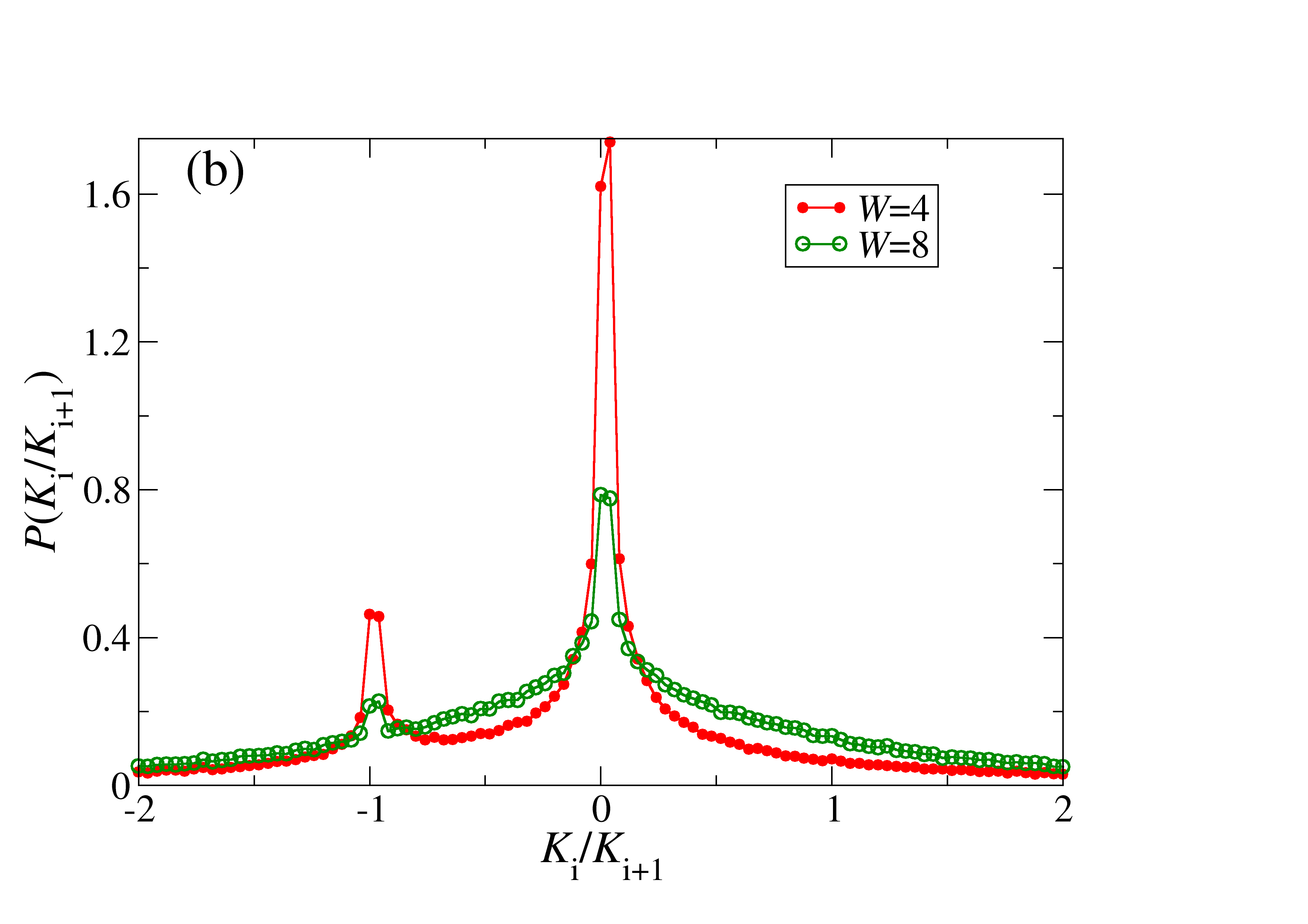 Figure 1
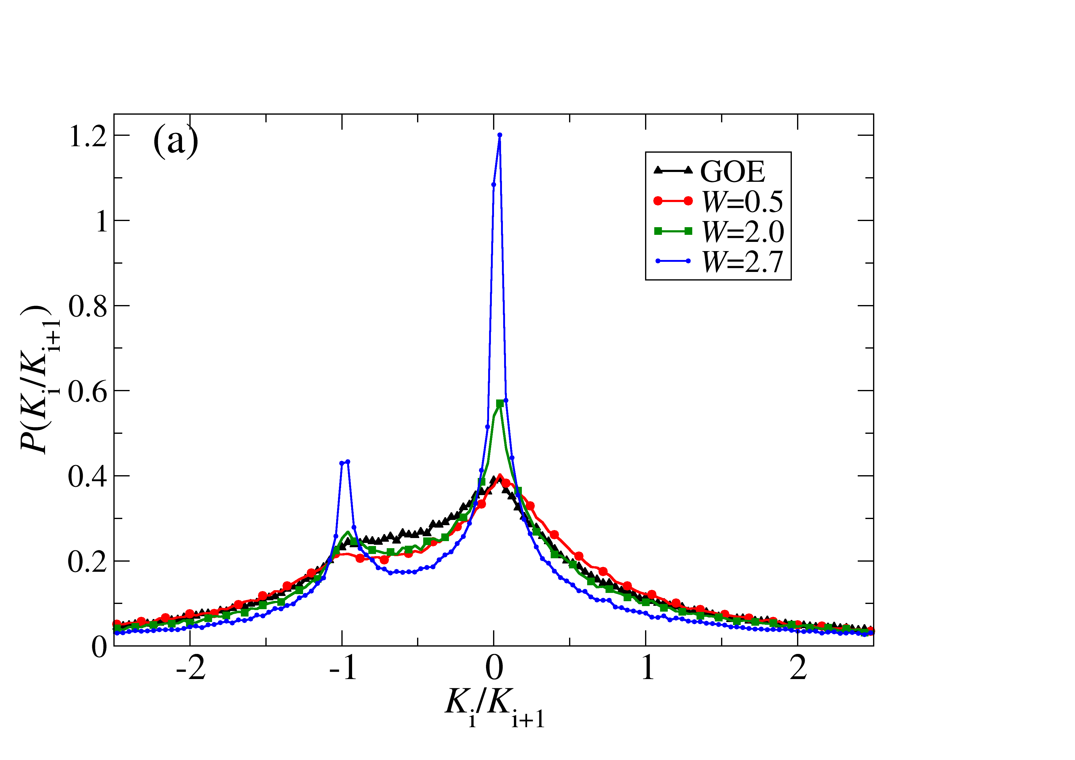 Figure 2
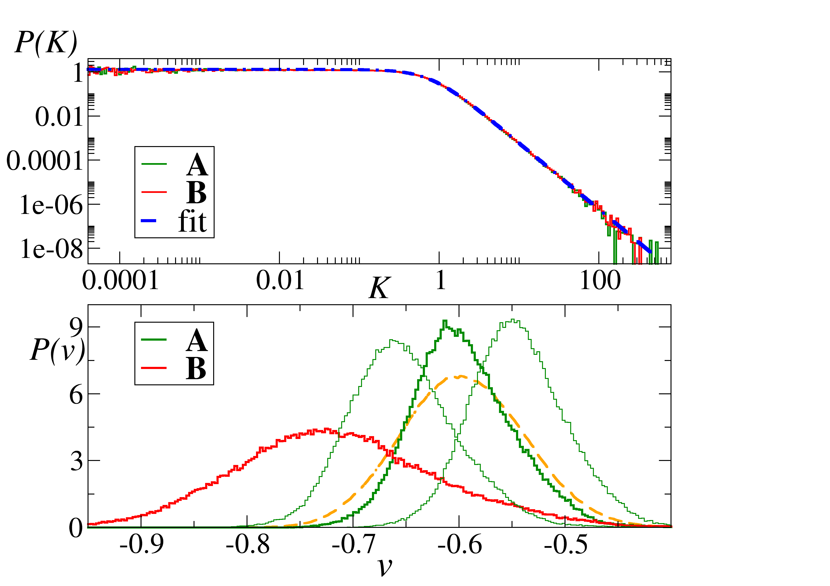 Figure 3
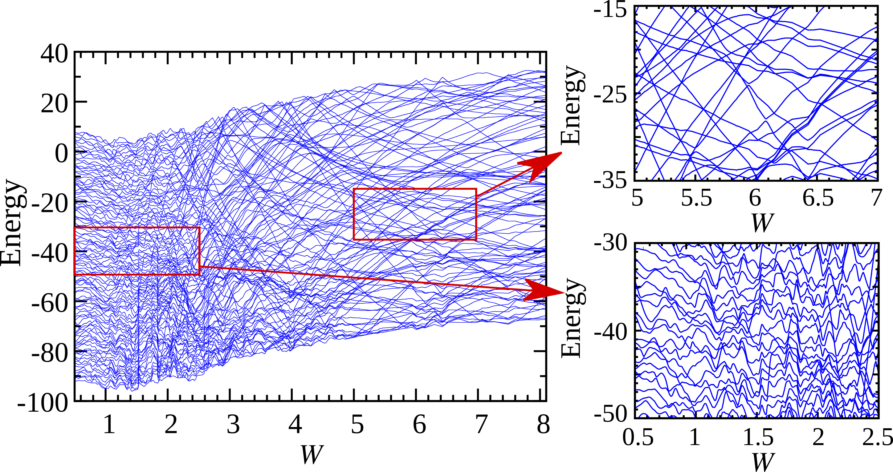 Figure 4
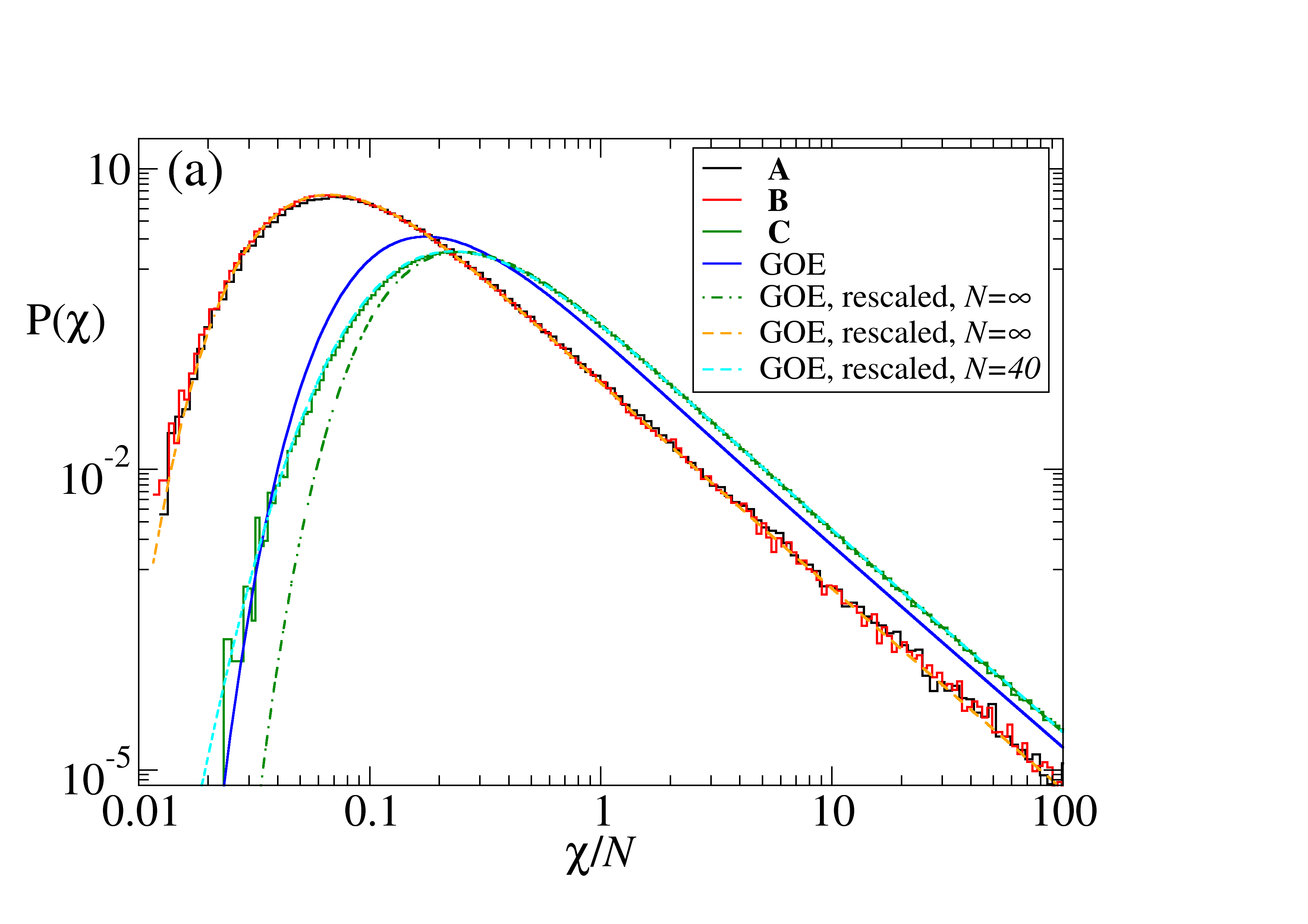 Figure 5
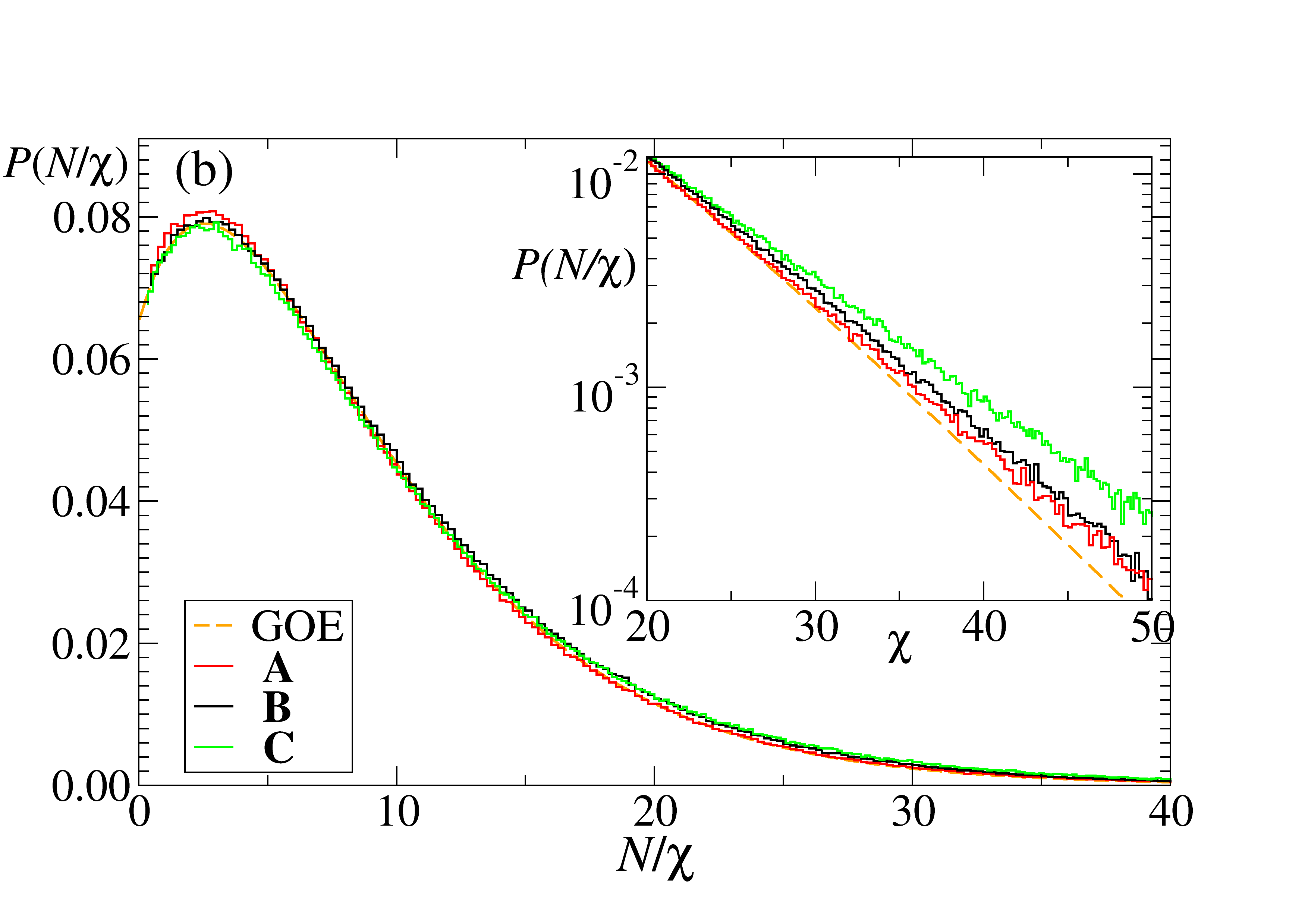 Figure 6
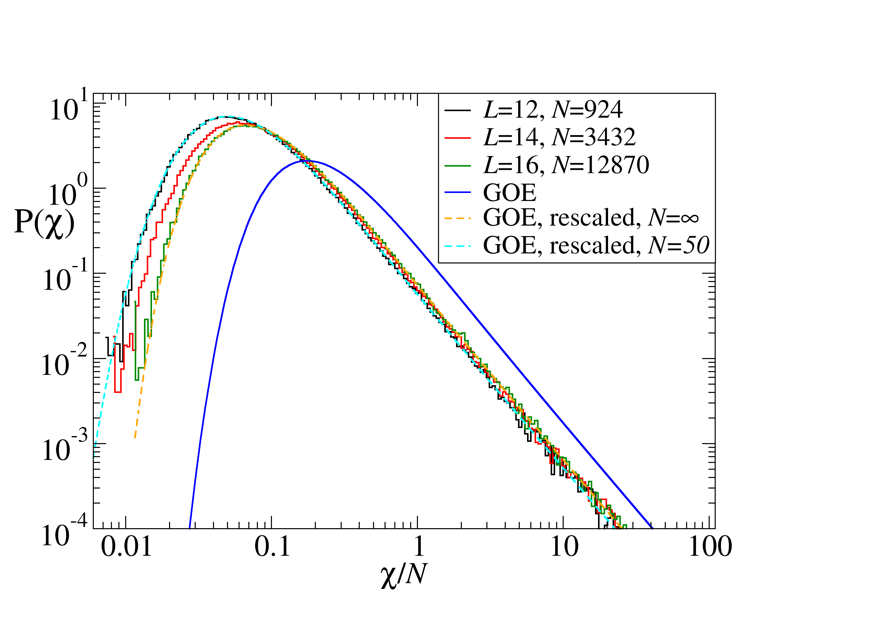 Figure 7
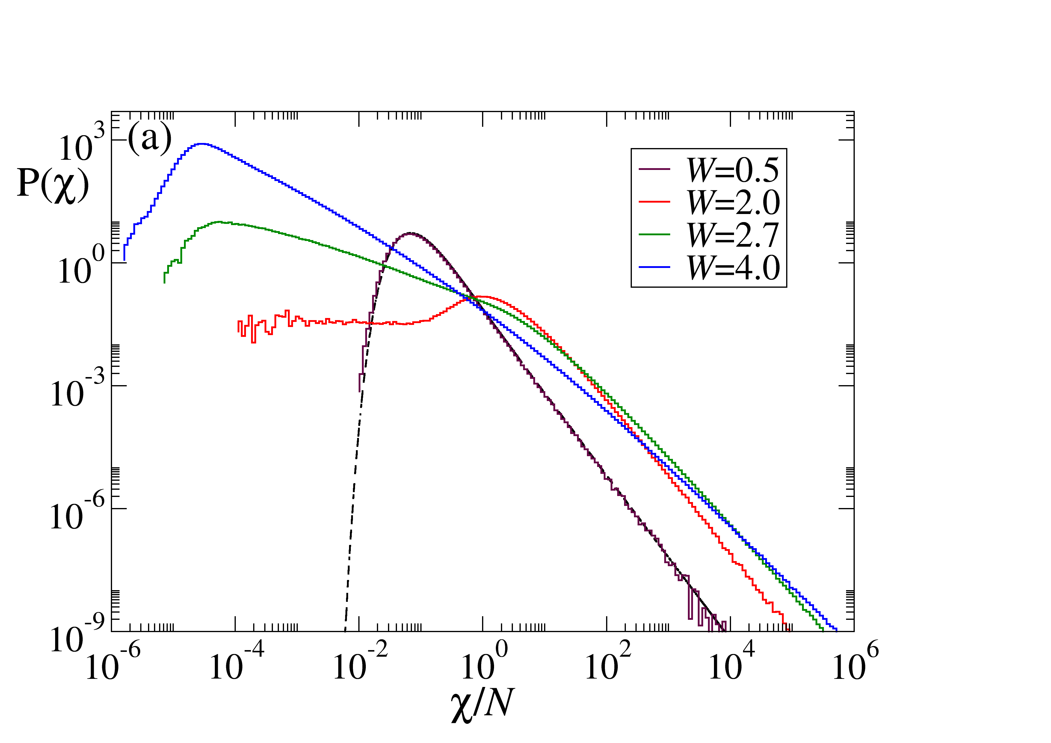 Figure 8
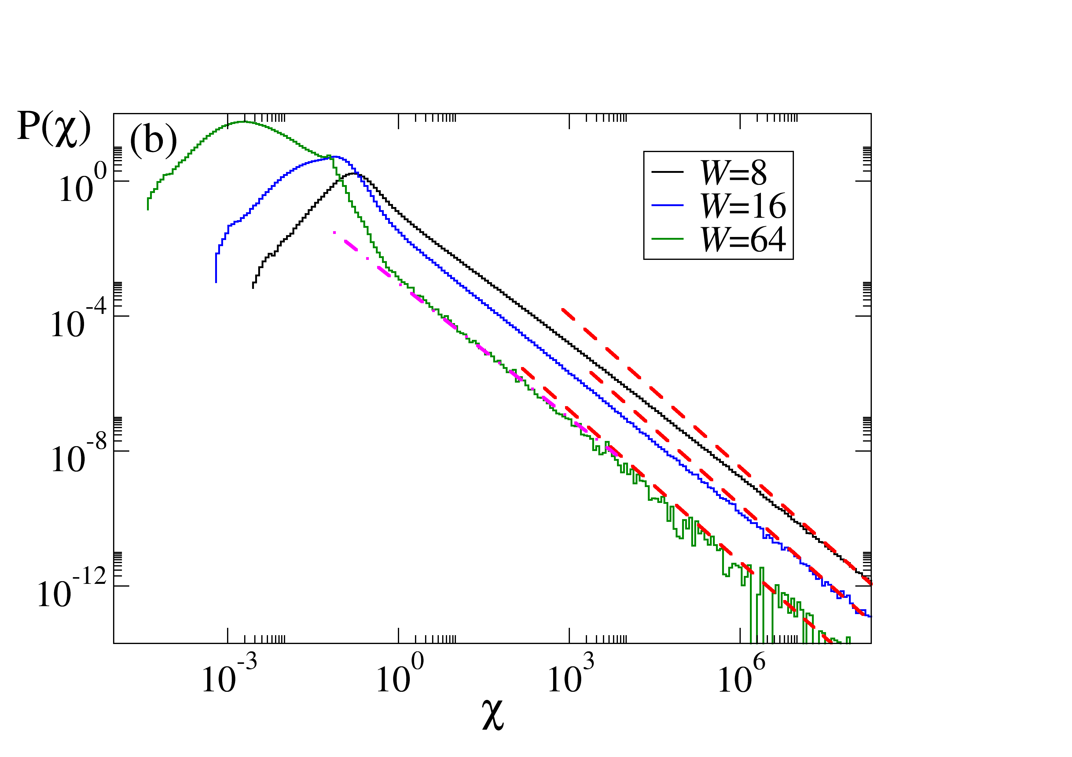 Figure 9
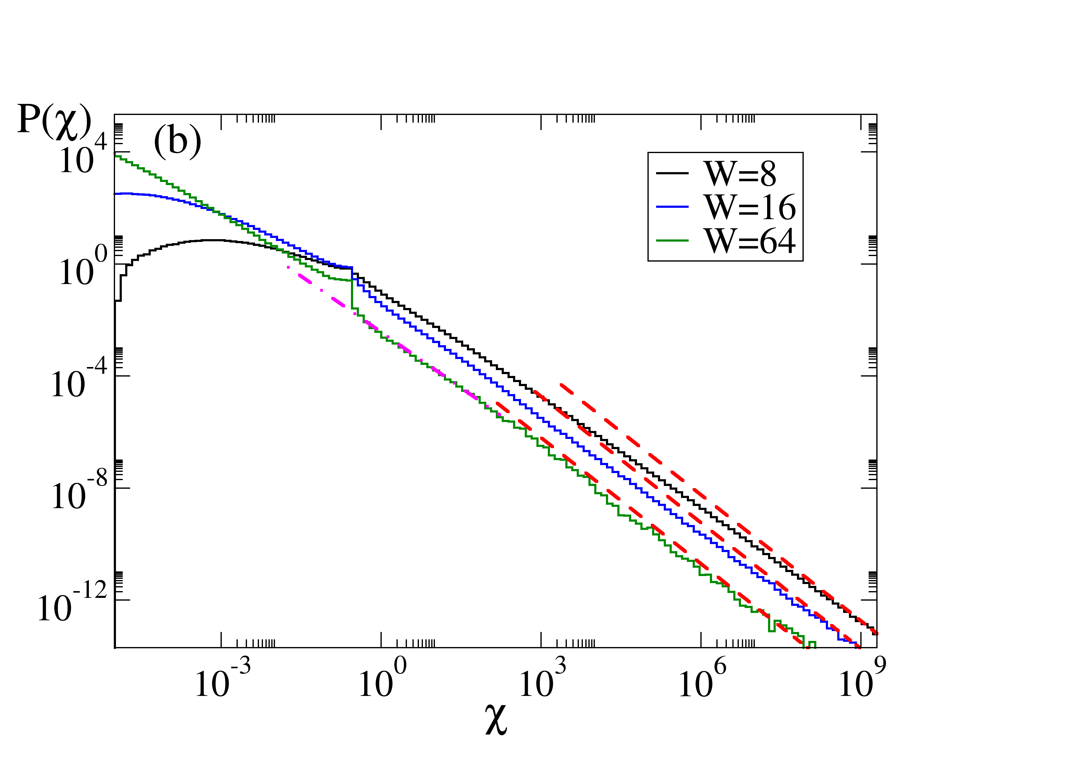 Figure 10
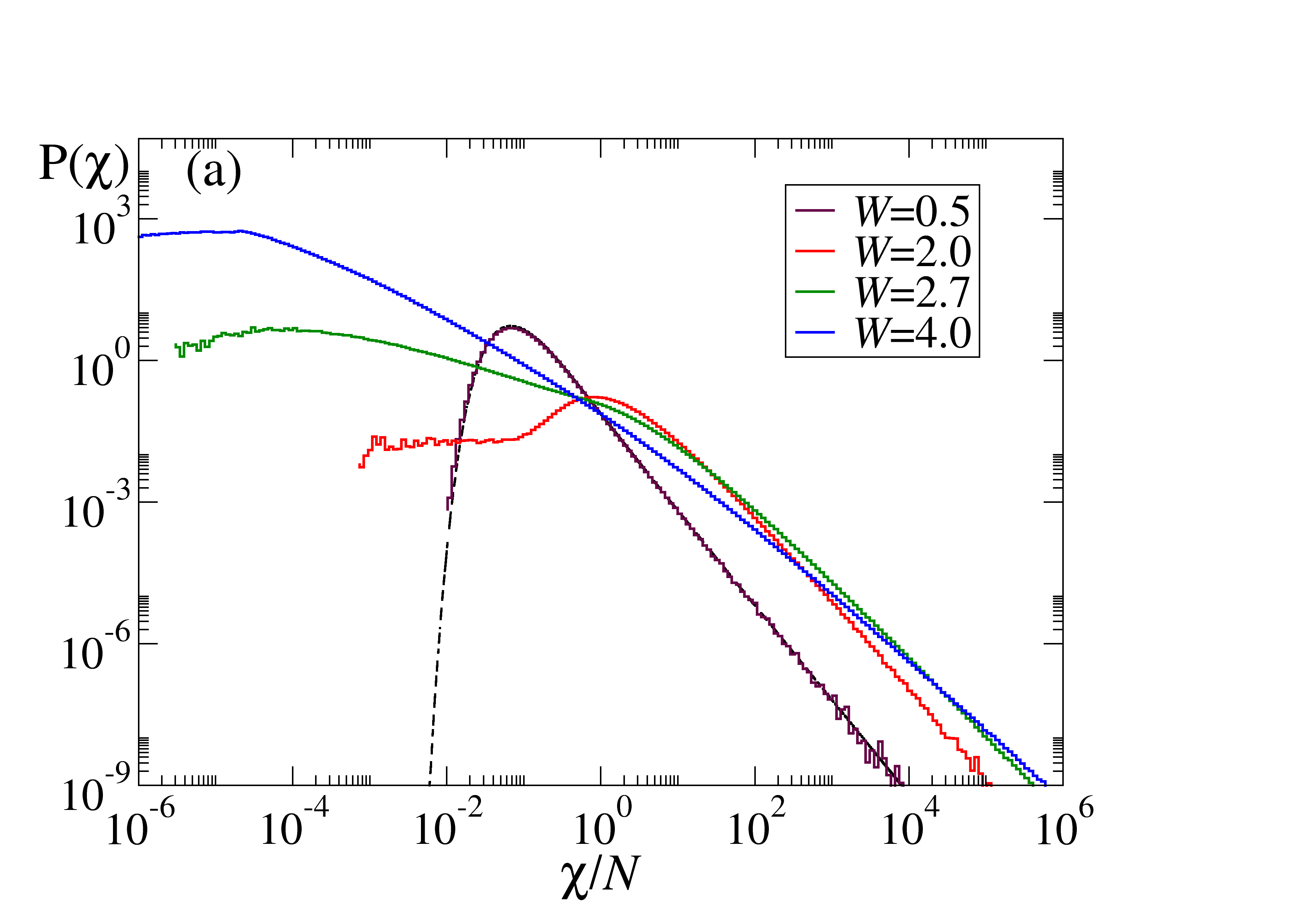 Figure 11
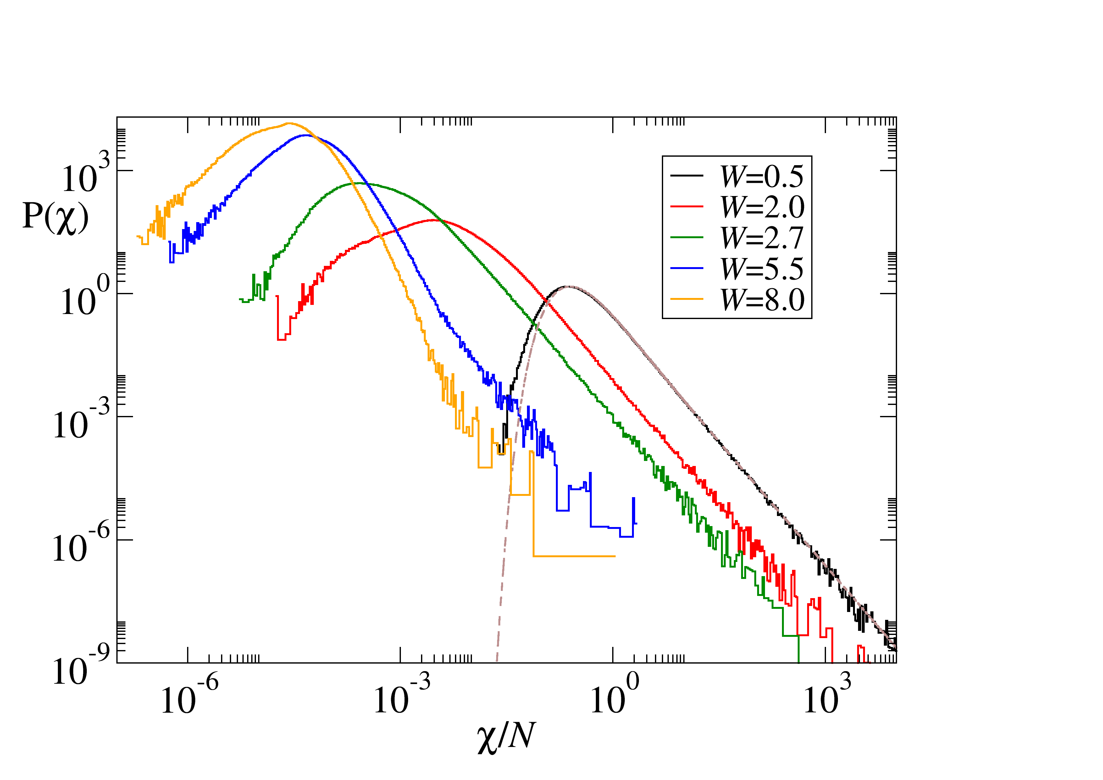 Figure 12
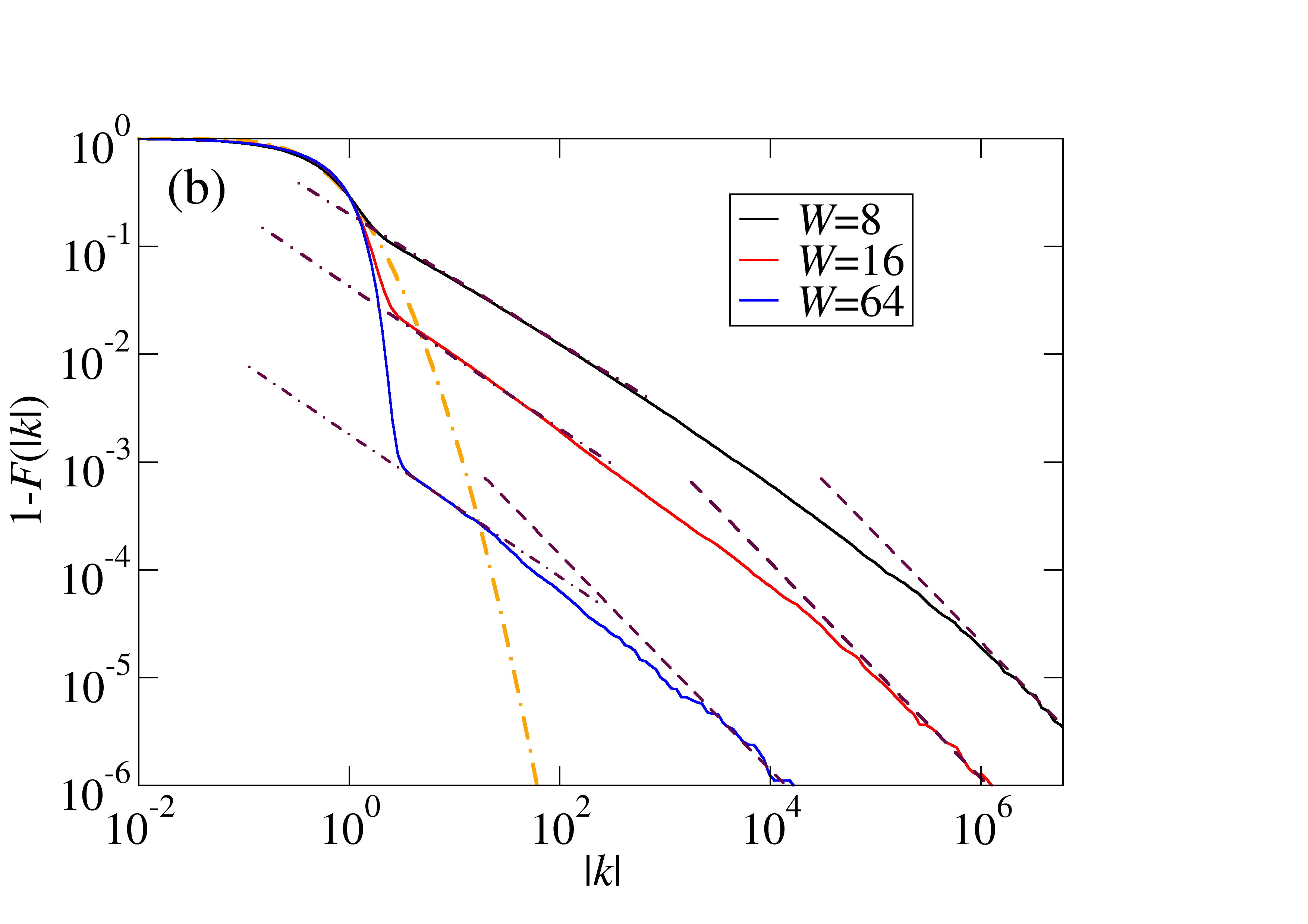 Figure 13
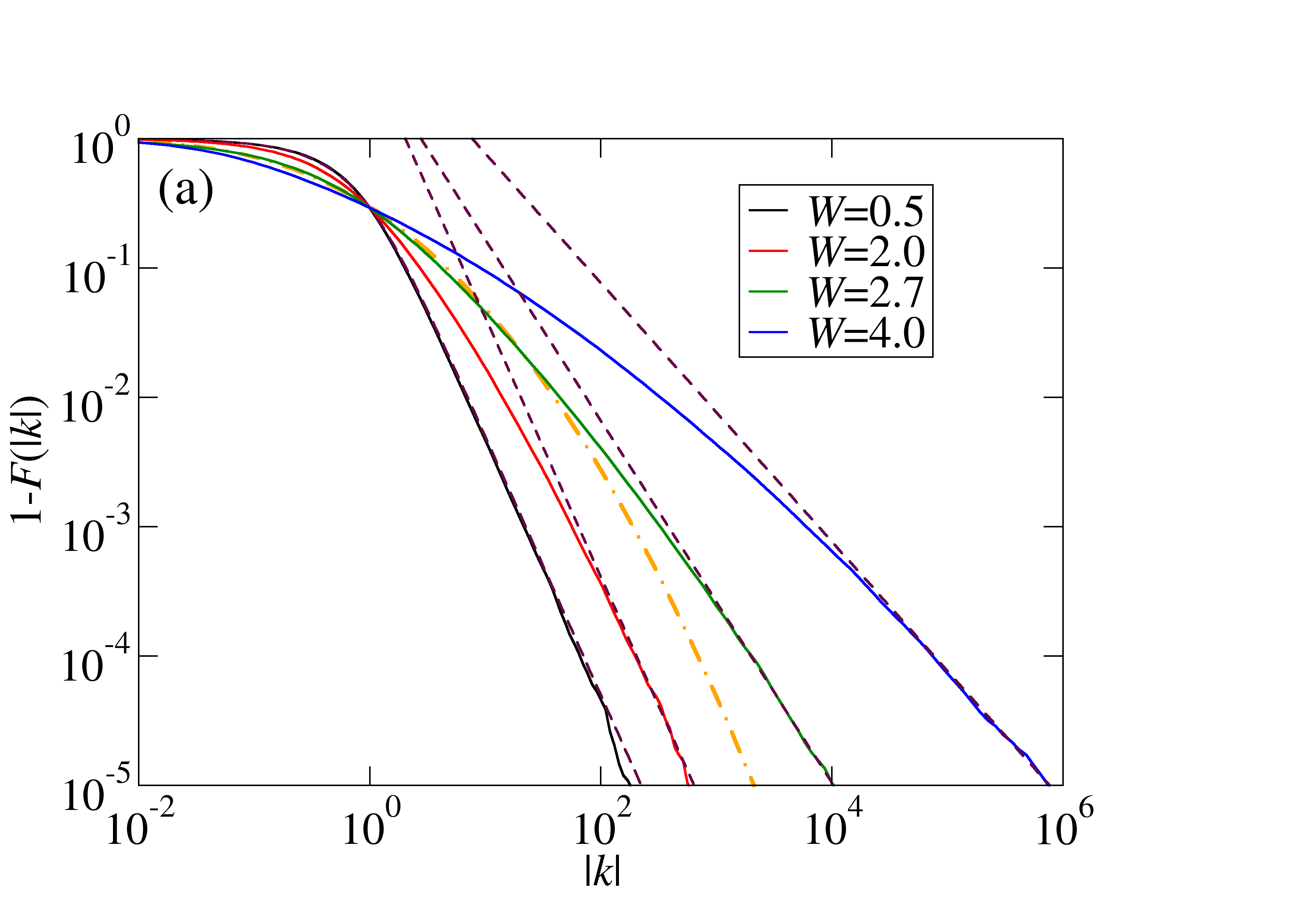 Figure 14
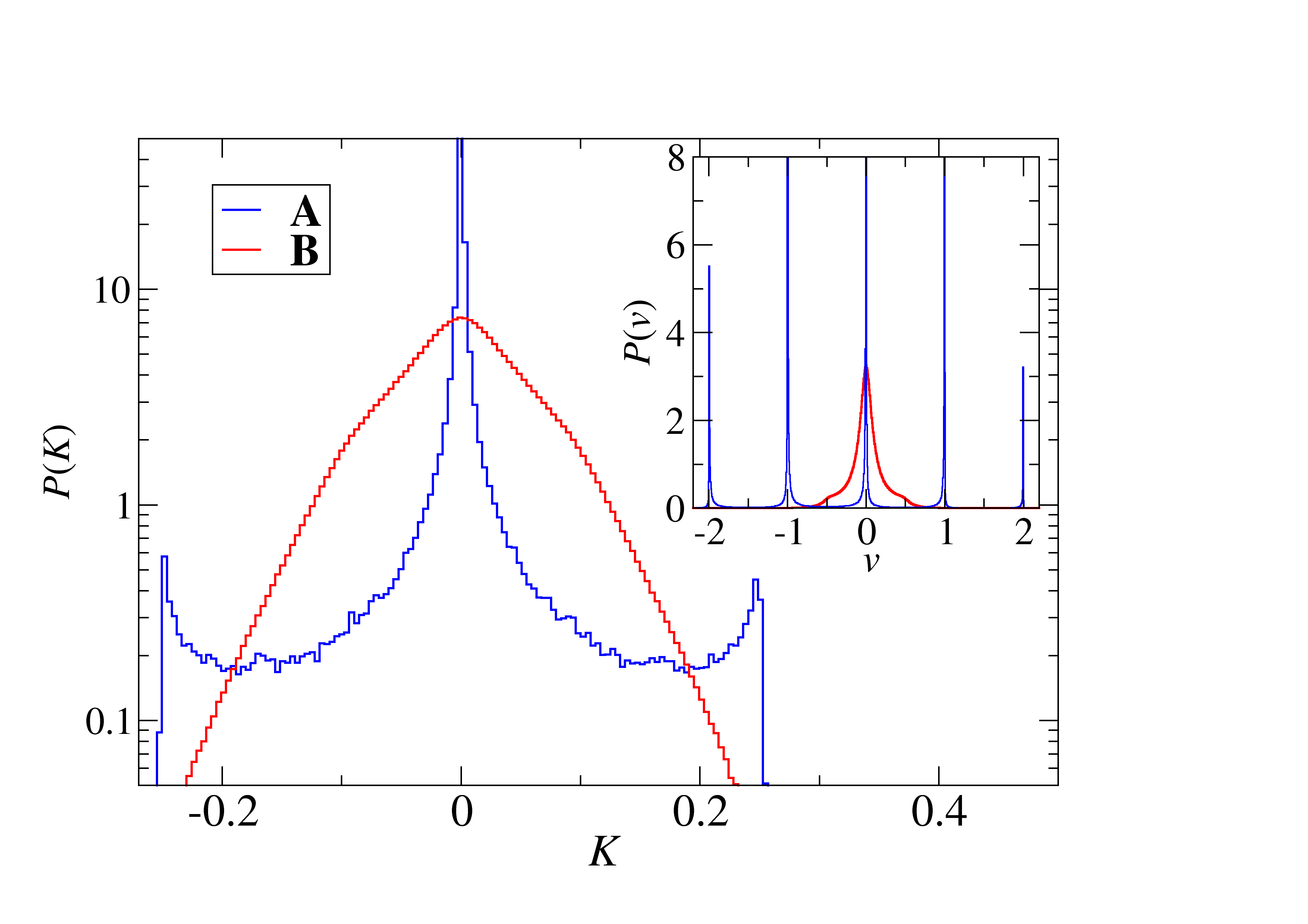 Figure 15
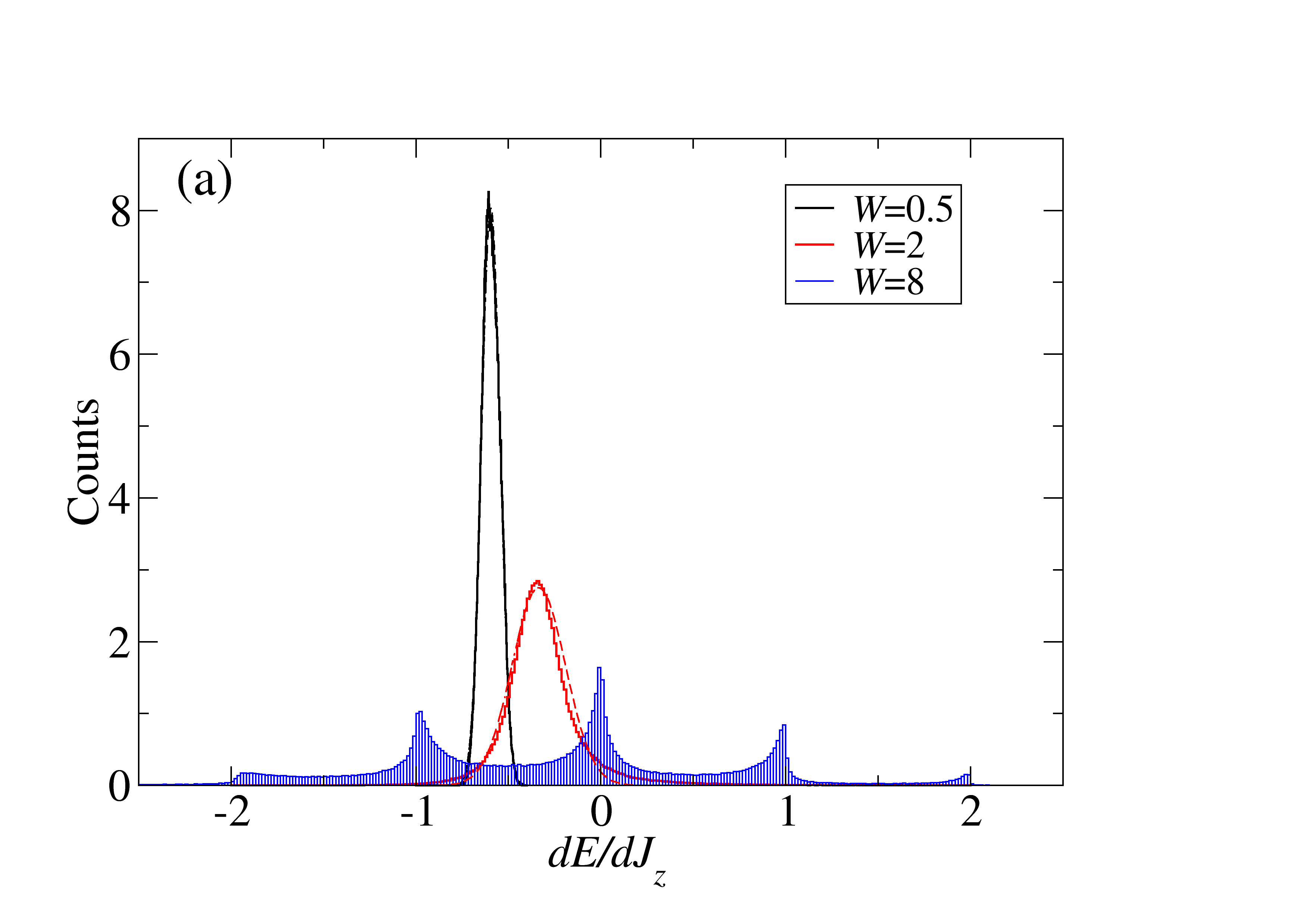 Figure 16
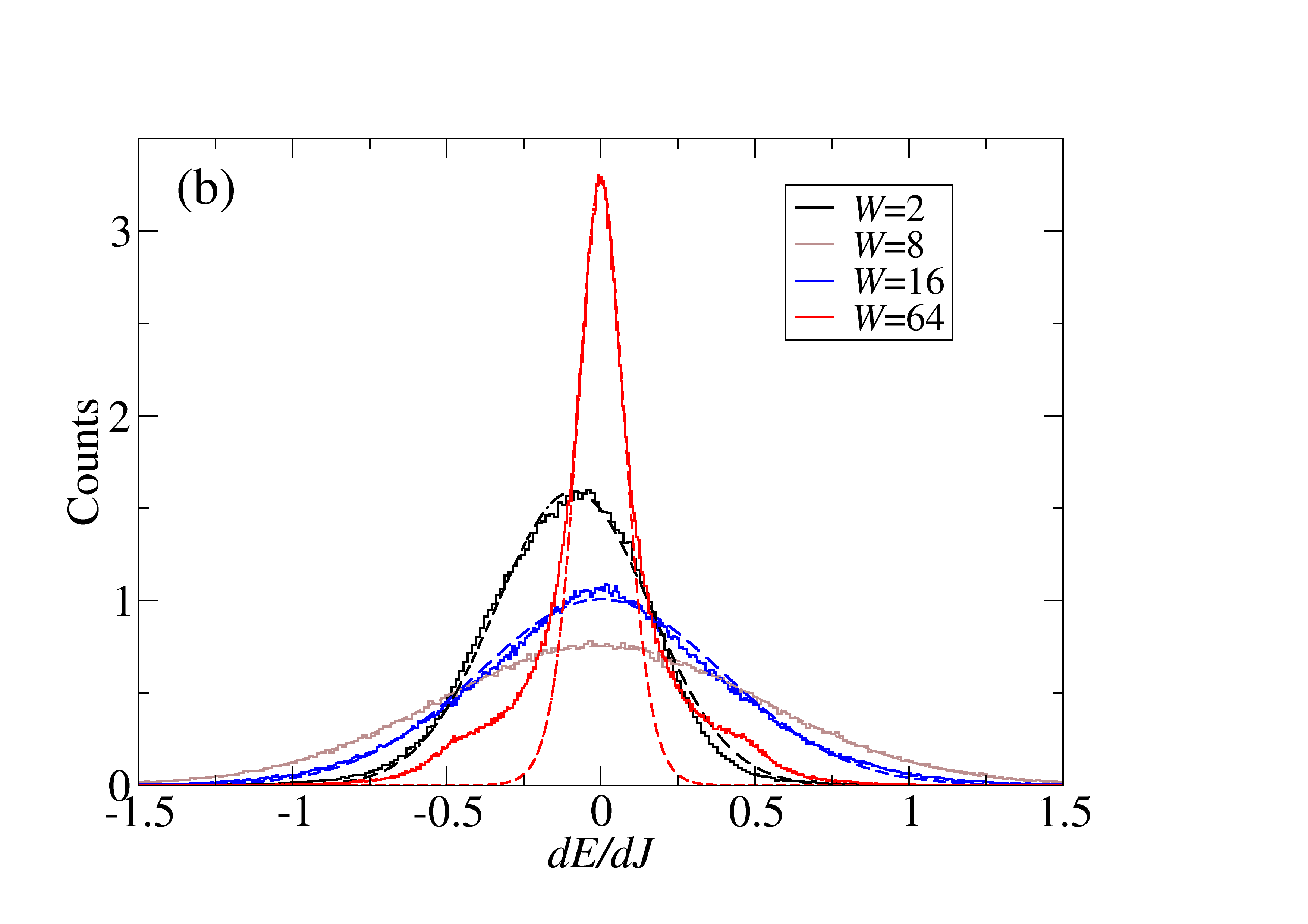 Figure 17
Peer Reviews
No public reviews on file for this paper yet. If you reviewed it on a platform where reviews are public (OpenReview, ICLR, NeurIPS, ICML), you can paste yours below so the community can read it here.
Videos
No videos yet. Explain this paper in a talk, walkthrough, or lecture? Add one.
Energy level dynamics across the many-body localization transition
Artur Maksymov
Piotr Sierant
Instytut Fizyki imienia Mariana Smoluchowskiego, Uniwersytet Jagielloński, ulica Łojasiewicza 11, PL-30-348 Kraków, Poland.
Jakub Zakrzewski
Instytut Fizyki imienia Mariana Smoluchowskiego, Uniwersytet Jagielloński, ulica Łojasiewicza 11, PL-30-348 Kraków, Poland.
Mark Kac Complex Systems Research Center, Uniwersytet Jagielloński, Kraków, Poland.
Abstract
The level dynamics across the many body localization transition is examined for XXZ-spin model with a random magnetic field. We compare different scenaria of parameter dependent motion in the system and consider measures such as level velocities, curvatures as well as their fidelity susceptibilities. Studying the ergodic phase of the model we find that the level dynamics does not reveal the commonly believed universal behavior after rescaling the curvatures by the level velocity variance. At the same time, distributions of level curvatures and fidelity susceptibilities coincide with properly rescaled distributions for Gaussian Orthogonal Ensemble of random matrices. Profound differences exists depending on way the level dynamics is imposed in the many-body localized phase of the model in which the level dynamics can be understood with the help of local integrals of motion.
I Introduction
Random matrix theory (RMT) based tools proved very effective in statistical analysis of quantum systems chaotic in the classical limit Bohigas et al. (1993); Haake (2010). One of the simplest measures is provided by level spacing statistics, Poissonian for integrable systems while revealing similarity with RMT predictions for chaotic models Bohigas et al. (1984); notably for time-reversal invariant systems solely addressed below, leading to an approximate Wigner surmise for the level spacing distribution.
The same measures proved fruitful for disordered systems. The spectrum of single particle, Anderson localized system has Poissonian character. In three dimensions, in the presence of disorder, systems may become delocalized with extended states and Wigner-type level statistics. The Anderson localization transiton attracted attention long time ago already, leading to first propositions of “intermediate statistics” Shklovskii et al. (1993) being again parallel to similar attempts to describe dynamical systems with mixed dynamics Lenz and Haake (1991).
With the development of many-body localization (MBL) the statistical description of localized and ergodic systems reached a new level. Already in the early days of MBL, Oganesyan and Huse Oganesyan and Huse (2007) introduced a new statistical measure, the so called gap ratio, which became a prime tool in a statistical analysis of many body spectra. It is defined as where is an energy difference between two consecutive levels. Being the ratio of two nearest spacings it is a dimensionless quantity, thus it may be determined without finding a local mean density of states and “unfolding” the spectra. As the unfolding procedure is not uniquely defined, the introduction of gap ratio was a major step simplifying statistical description of MBL related systems. The mean appeared as a simple and decisive measure of the statistical properties of many-body system with corresponding to Gaussian Orthogonal Ensemble (GOE) representing ergodic systems while corresponding to MBL situation with Poissonian level statistics Atas et al. (2013). Calculation of the average gap ratio allowed to localize the transition between ergodic and MBL phases in several models Oganesyan and Huse (2007); Luitz et al. (2015); Mondaini and Rigol (2015); Janarek et al. (2018); Wiater and Zakrzewski (2018); Sierant and Zakrzewski (2018); Sierant et al. (2019). The analysis of the transition with the more traditional level spacing distribution and related measures was performed in Serbyn et al. (2015); Bertrand and García-García (2016); Sierant and Zakrzewski (2019).
Level statistics provide, however, only information about eigenvalues of the Hamiltonian matrix which contains independent matrix elements. Thus, an additional insight into considered system may be gained by investigation of eigenstates. Their statistical description - e.g. via participation ratios, suffers, however, from the choice of the basis used for the analysis Durt et al. (2010). Here, as pointed out in a recent analysis of multifractality across MBL transition Macé et al. (2018) much less is known and open questions exist such as e.g. a possible existence of non-ergodic yet delocalized phase Pino et al. (2016); Torres-Herrera and Santos (2017); Luitz and Lev (2017); Pino et al. (2017) or the question of wavefunction properties in MBL regime Luca and Scardicchio (2013). These issues may be addressed by an analysis of generalized participation ratios Macé et al. (2018), an alternative approach is presented in the present work via the so-called “level response statistics” which characterizes the sensitivity of individual energy levels with respect to a change in the control parameter. Edwards and Thouless suggested in 1972 that the conductance of a disordered system may be related to the sensitivity of the spectrum to changes of boundary conditions Edwards and Thouless (1972). This led to level-dynamics studies, the early works Pechukas (1983); Yukawa (1985); Nakamura and Lakshmanan (1986) established a link with appropriate Gaussian random matrix theory (RMT) models. In level dynamics the role of time is taken by the parameter which is varied. Thus, e.g. energy level slopes, may be considered as velocities. The RMT leads then to Gaussian distribution of velocities (slopes). The velocity distribution ceases to be Gaussian when Anderson localization sets in – see Fyodorov (1994); Fyodorov and Mirlin (1995) where distribution of velocities in the localized regime has been proposed.
In the same spirit level curvatures defined as the second derivative of energy levels with respect to the parameter, were considered (we shall not call them accelerations despite the motion analogy). One of the earliest attempts to describe the curvature statistics for chaotic spectra was made by Gaspard in Gaspard et al. (1990). The analytical expressions for large curvatures limits were found for all three Gaussian ensembles: Gaussian unitary (GUE), orthogonal (GOE) and symplectic (GSE) ensembles and compared with numerics coming from model quantum chaos studies. The analytical expressions for curvature distributions were provided for all three ensembles on the basis of numerical studies Zakrzewski and Delande (1993):
[TABLE]
with for GOE, GUE and GSE respectively, where is normalization constant and the so called scaled curvature. It has been argued Simons and Altshuler (1993) that the scaling is universal with with in terms of the mean density of states, and the variance of the velocity distribution, . The astonishingly simple formula (1) was proven by von Oppen von Oppen (1994, 1995) – for a simple and instructive alternative derivation see also Fyodorov and Sommers (1995a).
Interestingly, the same formula (for GOE) was found to be applicable in the case of infinitesimal Aharonov-Bohm flux breaking the time reversal symmetry. The numerical findings Braun and Montambaux (1994) were confirmed analytically Fyodorov and Sommers (1995b).
The expression (1) describes the typical behavior of curvatures of quantally chaotic systems but already there one may observe deviations from universality as e.g. for stadium billiard or a paradigmatic model of quantum chaos – a hydrogen atom in a magnetic field. The nonuniversality features were related to eigenfunction scarring phenomenon Zakrzewski and Delande (1993) that modifies the small curvatures behavior. Curvature distributions in the Anderson localized case and in the transition between extended and localized regimes have been addressed in a number of works Casati et al. (1994); Fyodorov and Sommers (1995a); Canali et al. (1996); Titov et al. (1997); Braun et al. (1997); Zharekeshev and Kramer (1999); Evangelou (2004); Fyodorov (2011). For many-body system with infinitesimal Aharonov-Bohm flux the curvature distribution in the MBL regime was studied in Filippone et al. (2016).
Another related measure of sensitivity of a system to a change of a parameter is the fidelity, , defined as (note that often the square modulus is used for a definition – see discussion in Bengtsson and Życzkowski (2006)). For small enough one may expand the fidelity into Taylor series defining the fidelity susceptibility (the linear term in the expansion vanishes due to the wavefunction normalization). In a standard approach fidelity and fidelity susceptibility are evaluated for a small change of parameter for the ground state wavefunction. The latter undergoes dramatic changes at quantum phase transitions (QPT) reflected by a maximum of fidelity susceptibility at the critical point (or its divergence in the thermodynamic limit Zanardi and Paunković (2006); You et al. (2007)). Fidelity susceptibility is directly proportional to the Bures distance between density matrices corresponding to and Hübner (1993); Invernizzi et al. (2008) – this property can be extended to thermal states Zanardi et al. (2007); Sirker (2010); Rams et al. (2018). Let us note that universal information can be extracted from fidelity susceptibility in the vicinity of the critical points Campos Venuti and Zanardi (2007); Zhou et al. (2008); Schwandt et al. (2009); Albuquerque et al. (2010); Gu (2010); Rams and Damski (2011a, b); Damski (2013); Damski and Rams (2014).
For MBL all states are important so one can introduce fidelity (and fidelity susceptibility) of excited states as well (not being limited to thermal states). In an interesting approach Hu et al. (2016) it was shown that fidelity of specially prepared state (the so called diagonal ensemble) may signal MBL transition. We shall consider an entire fidelity susceptibility distribution for all quantum states of the system, also for generic random matrix representations of Hamiltonians. Recently, analytic predictions for fidelity susceptibility distribution for GOE/GUE dynamics have been derived analytically Sierant et al. (2019). We shall consider how this distribution is affected when entering then MBL regime.
For completeness, let us mention yet another measure of level dynamics, the distribution of avoided crossing sizes relevant for situations when a change of parameter is aimed at being adiabatic. It has been studied in a number of works for chaotic systems also in the spirit of RMT Wilkinson (1989); Zakrzewski and Kuś (1991); Zakrzewski et al. (1993).
As mentioned above, level dynamics provides a complete (via the formalism of Pechukas (1983); Yukawa (1985); Nakamura and Lakshmanan (1986)) access to properties of not only eigenvalues but also matrix elements in the eigenstate basis of different physical operators. This paves a way to a more comprehensive understanding of MBL which, despite years of studies, remains a controversial phenomenon Šuntajs et al. (2019). The present contribution makes the first step in this, hitherto practically unexplored direction.
The paper is organized as follows. First, we provide a brief review of level dynamics as typically considered in quantum chaos studies. Then, we discuss velocities, curvatures, and fidelity susceptibility distributions first in the delocalized then in the localized regime. Most surprizingly, we find that in the delocalized regime the level dynamics indicates signatures of nonuniversal behavior. In the localized phase we show that the system sensitivity to perturbation is strongly dependent on the perturbation itself indicating a connection with description of MBL system in terms of the so called Local Integrals of Motion (LIOMs) Huse et al. (2014); Serbyn et al. (2013). Finally, we discuss the results and provide future perspectives.
II The level dynamics revisited
Let us revisit a simple picture of level dynamics. Consider a general Hamiltonian . The particular form often assumed is but we do not limit ourselves to this particular choice. The Schrödinger equation reads
[TABLE]
Differentiating this equation side-wise with respect to , and taking the left product with we obtain (where the is a substitution for )
[TABLE]
where (hereafter the hat is omitted for convenience). In a particular case of dynamics suppose that belongs to GOE (GUE). Then for generic from the same ensemble its diagonal elements in the basis of eigenvectors are Gaussian distributed giving trivially the Gaussian level “velocity distribution” for GOE (GUE).
The situation is more complicated for curvatures . Differentiating (3) we get
[TABLE]
where we used the resolution of unity. Again differentiating (2) but now taking the left product with for we get
[TABLE]
which placed in (4) gives the standard expression for the level curvature
[TABLE]
The first term vanishes for scenario. In particular, for and belonging to GOE (GUE) ensembles one may easily derive a relation between large curvature tail of curvature distribution, , and the spacing distribution, . For generic the matrix elements in the numerator of (6) are independent of the denominator. Large corresponds to small . Thus for large . If for small behaves as ( for GOE, GUE respectively) then for large Gaspard et al. (1990). As mentioned in the Introduction after appropriate rescaling an exact expression for curvature distribution (1) is available Zakrzewski and Delande (1993); von Oppen (1994); Fyodorov and Sommers (1995a).
Similarly the fidelity susceptibility may be expressed as
[TABLE]
The analogous argument to that for curvatures Monthus (2017) gives the large tails of the fidelity susceptibility distribution as .
Let us note that the similar arguments gives large curvature and fidelity susceptibility tails for integrable (e.g. localized) case where is Poissonian. One may expect and tails of the corresponding distributions assuming that the spacings are independent from matrix elements of the perturbation Monthus (2017). For curvatures it is in apparent contradiction with the log-normal distribution postulated in deeply localized regime Titov et al. (1997).
III The model
We consider XXZ model Hamiltonian – the paradigmatic model of MBL transition Mondaini and Rigol (2015)
[TABLE]
where are spin- degrees of freedom at site , and are the coupling strengths for XY and Z components respectively, is the random magnetic field drawn from an appropriate distribution. Typically one considers a random uniform distribution in interval where is the disorder strength. The Hamiltonian (8) maps directly to interacting spinless fermion model:
[TABLE]
where () are fermion annihilation (creation) operators at site with being the occupation at site . In this picture corresponds to the tunneling and is the interaction strength.
There are several ways how one can introduce the parameter change in the problem. One may vary the tunneling affecting XY coupling in the spin Hamiltonian. Alternatively, one may modify – interaction strength in the fermion picture. It is also possible to modify random on-site couplings. The example of such a change is shown in Fig. 1. Finally, Thouless suggested Edwards and Thouless (1972); Thouless (1974) that the average conductance is proportional to the width of the curvature distribution (where the parameter changed, , is a small twist of the boundary conditions). Explicitly, the tunneling term of (9) takes then the form
[TABLE]
Such an approach was applied in the early study of localization in banded random matrices Casati et al. (1994) and was frequently used for different systems approaching Anderson localization Fyodorov and Sommers (1995a, b); Canali et al. (1996); Titov et al. (1997); Braun et al. (1997); Zharekeshev and Kramer (1999); Evangelou (2004); Fyodorov (2011). For 1D disordered systems the log-normal distribution of curvatures is postulated in the localized regimeTitov et al. (1997); Evangelou (2004) although the deviations from it are indicated in some works Casati et al. (1994). Observe that the twist of boundary conditions (passing to the moving frame) explicitly breaks time-reversal invariance in the system, so such an approach may exhibit different features than changing of and which keeps the system within the same universality class.
The qualitative picture of the system behavior at different values of the disorder amplitude is shown in Fig. 1. Here and in the following all parameters of the problem with the dimension of energy are expressed in units of the tunneling (thus , when we study level dynamics changing , small changes of will be considered around this \c@). The spectrum of a small (for clarity) exemplary system is plotted for a single random realization of disorder. Enlarged areas depict two characteristic regions. Small values correspond to delocalized, ergodic regime with a characteristic large number of avoided crossings (with their sizes being Gaussian distributed for the appropriate GOE universality class Zakrzewski et al. (1993)). For larger , a transition to a different localized regime occurs (where integrability is assured by the existence of Local Integrals of Motion (LIOMs) Huse et al. (2014); Serbyn et al. (2013)). There the avoided crossings are replaced by crossings of levels that are an apparent manifestation of the existence of LIOMs.
For our system we shall introduce the following level dynamics
A. The perturbation is given by (the second expression in the spin language) thus interaction strength is modified;
B. The perturbation is given by - thus tunneling term is affected;
C. Twisted boundary conditions in the form of (10) are assumed.
IV The delocalized, almost GOE regime
IV.1 Velocities and Curvatures
MBL transition occurs in the studied XXZ spin chain at Luitz et al. (2015). As representative value of disorder strength in the ergodic regime we choose for which , staying away from the crossover regime which starts at for system size and also from the integrable point at . To see how the predictions of universal level dynamics Simons and Altshuler (1993) are fulfilled let us review its basic findings. In essence, the level dynamics should depend on a single parameter – the variance of the level velocities defined as where denotes average over disorder realizations. This implies, in particular, that the curvature distributions, regardless of the perturbation should be described by (1) if rescaled appropriately by the velocity variance.
Fig. 2 reveals that it is not the case. The top panel shows that unscaled curvatures for both and perturbation, whereas the bottom panel shows the respective velocity distributions . Firstly, the velocity distributions are not Gaussian as one would expect for GOE but rather are visibly asymmetric. Moreover, the number of velocities taken from each disorder realization (from the center of energy spectrum) plays unexpectedly important role. The number of energy levels for which the average gap ratio remains , is way above of the total Hilbert space that corresponds to eigenvalues from the middle of the spectrum. We observe, however, that the velocity distribution approximates well a distribution for a single level at the band center only for . Shifting the position of the interval from which velocities are taken by of the dimension of Hilbert space does not affect but results in a significant shift of the as demonstrated on example of B perturbation in Fig. 2. Taking velocities from the middle of the spectrum results in drawn by the dashed line – with a significantly larger variance . It is thus crucial to consider for not larger than for . This however leads us to an unexpected result.
Since the velocity distributions corresponding to perturbations A and B are vastly different with significantly different variances and since distributions overlap for the two cases, the scaled curvature distributions differ. This is a clear indication of a nonuniversal behavior of XXZ Hamiltonian as far as level dynamics is concerned in the ergodic regime. The unscaled curvature distribution agreement must be interpreted as accidental. Suppose we reshape the perturbation as with and . Then unscaled curvatures calculated with respect to are smaller then the original ones. As the same scaling occurs for the velocity variance the scaled curvatures are not affected by such a transformation.
Still, in both considered cases, after rescaling properly curvatures by the factor suggested by RMT, i.e. , the distribution obtained does not coincide with (1), simply does not yield a proper width. Let us note, however, that the distribution is very well reproduced by (1) provided a width of the distribution is fitted, instead of being defined by the velocity variance – compare Fig. 2.
The surprising, nonuniversal behavior is robust in the sense that it occurs also for systems with different disorder amplitude (sufficiently small to be far from the transition to the localized regime). Similarly it is robust to changes of Hamiltonian. For instance, we have added the next neighbors tunnelings assuring that system remains nonintegrable (quantum chaotic) at (following Oganesyan and Huse (2007)). This leads to a similar, nonuniversal behavior. On the other hand, consistently, we find that the curvature distribution is faithfully represented by (1) provided the width of the distribution is determined by a fit and not by the velocity variance.
The same distribution works well also for the twisted boundary conditions, case C as shown already in Filippone et al. (2016). In that case all velocities vanish identically due to the symmetry of the Hamiltonian, so the width of the distribution remains a sole parameter of the fit.
IV.2 Fidelity
The fidelity susceptibility distribution has not been studied before for any physical system. It seems, therefore, even more interesting to inspect the numerical data for this measure for different perturbation schemes. Let us recall that there exists an analytic prediction for the fidelity susceptibility, , distribution, as a function of for GOE and GUE Sierant et al. (2019) with being the matrix rank. Fidelity susceptibility distribution for GOE matrices in limit reads
[TABLE]
Let us consider the rescaling of the perturbation parameter, in the form corresponding to the perturbation change with . The very definition of the fidelity susceptibility, via a Taylor expansion shows that a transformation to rescales fidelity susceptibility by a factor of . The analytic prediction derived in Sierant et al. (2019) assumes the same density of states both for the original Hamiltonian and its perturbation . Since we do not intend to estimate the energy scale of the perturbation we add a scaling factor (playing the role of an effective width) defining with
[TABLE]
As an example consider first the perturbation of tunnelings, i.e. the B case. The corresponding data are shown in Fig. 3 and compared with the GOE prediction Sierant et al. (2019). The GOE prediction (11) seems to be a bad choice at the first glance but after rescaling the universal prediction, (12), represents well the numerical data for the largest considered system size, . A significant discrepancy at small fidelity susceptibilities is visible between formula (12) and data for . To resolve this issue we use the exact formula for fidelity susceptibility distribution for GOE matrix of size Sierant et al. (2019)
[TABLE]
where is a normalization constant, is assumed to be even. Defining appropriately rescaled , we find that the data for are very accurately reproduced if one assumes in (13). This result indicates that B (tunnelings) perturbation of the XXZ spin chain Hamiltonian (8) on sites (with Hilbert space dimension ) generates the same fidelity susceptibility distribution as level dynamics within GOE ensemble of matrices with , much smaller than the dimension of the Hilbert space.
Fig. 4a compares the fidelity susceptibility distributions obtained for all three perturbations for system. Type A and B perturbations practically coincide, both perturbations preserve time reversal invariant symmetry and apparently the width reflecting the effective energy scale of perturbation is similar. On the other hand, the green curve in Fig. 4 left panel shows the fidelity susceptibility distribution for the twisted case C. The scaling is remarkably different but this is not surprising as the perturbation is vastly different. A clear deviation from (12) is observed for small fidelities that can be taken into account by considering (13) with . Note that in this case, the ratio of dimension of Hilbert space and of size of matrices from GOE which reproduce the fidelity susceptibility distribution is much larger than for and B perturbation. The perturbation C breaks the time reversal invariance so it is not obvious to what extent (12) and (13) distributions are applicable.
While has a rather complicated form, (12) a much simpler distribution is obtained looking at the inverse variable, . Explicitly
[TABLE]
revealing an exponential tail for large (i.e. small fidelities). The suppression of small fidelity susceptibilities in GOE-dynamics is expected due to strong level interactions. Fig. 4b shows for all three perturbations considered. The corresponding widths are adjusted and deviations from GOE-like behavior (14) are observed in the tails of the distributions. The differences between resulting fidelity susceptibility distributions for the three perturbations are an another manifestation of nonuniversality of level dynamics in the ergodic regime.
IV.3 Partial summary - delocalized regime
Before investigating the transition towards MBL it is worthwhile to summarize the quite surprizing findings we uncovered in the delocalized regime. Contrary to claims Macé et al. (2018) that this regime is purely ergodic as indicated by the appropriate fractal dimension obtained from the participation ratio, we have observed a clear breakdown of the universality of level dynamics as expected for systems faithful to random matrix theory predictions. Matrix elements of different operators, appropriate for level velocities for different perturbations, lead apparently to nonuniversal behavior of level dynamics. Thus, apparently, the considered exemplary system is quite sensitive to the way in which it is perturbed despite showing eigenvalue statistics that is in a full accord with GOE.
V Transition towards many-body localized regime
With increasing disorder strength, , the system undergoes a transition to MBL regime. The transition is expected to occur at Luitz et al. (2015) in thermodynamically large system. A crossover between the ergodic and MBL behaviors is observed at finite system size . For relatively small system sizes amenable to exact diagonalization, a characteristic value of disorder strength for which inter-sample randomness in the system is maximal Sierant and Zakrzewski (2019) is for (and in the thermodynamic limit).
It is interesting to investigate how different measures of level dynamics change across this ergodic-MBL crossover. We shall consider here separately velocities, curvatures and fidelities – that will allow, we hope to elucidate on the character of the transition as well as on the MBL phase properties.
V.1 Velocities
Here we may compare only velocities for an “interaction” perturbation A with those for a “tunneling” perturbation B as velocities for C case vanish identically due to symmetry considerations. In the deeply delocalized regime for small disorder, we have seen that both velocity distributions were almost Gaussian (with, however, non-negligible skewness, see the bottom panel in Fig. 2).
Fig. 5 shows numerically obtained distributions of velocities for both types of perturbation. On the delocalized side and across the MBL transition both perturbations result in almost Gaussian distributions with widths increasing with the disorder strength, . In the MBL phase the velocity distributions become markedly different. In particular for “interaction” perturbation a multi-peak structure appears – compare Fig. 5a. While quite suspicious at first glance (with peaks localized approximately at integer values of velocities) this surprising structure may be quite easily understood taking into account the character of the perturbation which reads, recall . Thus velocities are nothing else that the average of . In the MBL phase, there exists a set of LIOMs localized on different sites – those are just “dressed” operators. Thus are almost diagonal in the eigenbasis of , each element of the sum giving approximately . Within the subspace for we have eight pairs thus dominantly yielding as velocities. For slightly smaller system we would have then as dominant contributions – and indeed this is the result (not shown).
Fig. 5b shows the velocity distribution for “tunneling” perturbation B. As in the previous case we observe that in the ergodic regime with an increase of we observe broadening of the velocity distribution which is quite well represented by the Gaussian shape. For this perturbation the Gaussian shape persists at but going deeper into the localized regime we observe first narrowing of the distribution and then strong deviations from the Gaussian shape. The distribution for deeply localized regime attains quite complicated shape. Interestingly, the central, dominating peak may be quite well reproduced (see red dashed line) by the velocity distribution analytically derived Fyodorov (1994) in the framework of a nonlinear sigma-model for a disordered 1D wire in the localized regime and given by
[TABLE]
V.2 Curvature distribution
Let us consider now curvature distributions. Immediately, we face the problem of an appropriate scaling of curvatures. We shall apply here the idea introduced in Filippone et al. (2016), where instead of curvature distribution its cumulative distribution is concerned. It is defined as
[TABLE]
where is the distribution of unscaled curvatures for a given set. The width of the distribution, is defined as a value of such that . It has been found in Filippone et al. (2016) that it is important, in the localized regime, to find the appropriate width for each realization of the disorder, find rescaled curvatures and then combine distributions from different disorder realizations. This reduces the errors Filippone et al. (2016) as compared to calculating the width of whole sets corresponding to all realizations. Indeed we have confirmed that the difference may be significant in the localized regime also for our data, so the results presented are obtained with the former approach as in Filippone et al. (2016). For this reason we do not present data for Aharonov-Bohm flux case discussed in Filippone et al. (2016) commenting only that our results are fully consistent with that work. Instead we concentrate on perturbations A and B corresponding to level dynamics in a time reversal invariant system.
Fig. 6 shows the integrated curvature distributions obtained for the “tunneling” perturbation B. The left panel presents the data in the transition between ergodic and MBL regime. The curvature distribution (and its integral, , depicted in the figure) retains the algebraic tail for large curvatures, with, however smoothly changing with increase of . In this regime the data for “interaction” perturbation A exactly match those for perturbation B despite the fact that velocity distributions differ.
The situation changes in deeply localized regime as shown in the right panel again for perturbation B only. The obtained distributions seem to correspond to two types of levels. Levels in the first group are characterized by small curvatures – large curvatures are exponentially avoided. On the other hand there remains a fraction of levels with large curvatures and algebraic tail of the integrated distribution. The corresponding power (see dashed lines in the figure) changes smoothly between and at very large . Note, that with increasing the first group grows while the second group of levels shrink. For the algebraic behavior corresponds to at most a “permille” of all curvatures collected.
On the other hand the distribution of rescaled curvatures in the localized regime for A perturbation shows strange irregularities. Inspection of single realizations reveals that few distinct values of curvatures appear, most notably vanishing curvatures are abundant. This suggests that energy levels form straight lines as a function of the parameter. Moreover, we have seen already in Fig. 2 that velocities for the type A perturbations are peaked at distinct values. In effect, the statistics of curvatures for A perturbation does not bring other interesting information except the fact that levels are organized in groups of very similar velocities – compare the inset in Fig 7. Levels within the group have predominantly very small curvatures as exemplified in the main panel of Fig 7. Only when levels corresponding to different velocity groups cross, the resulting narrow avoided crossings lead to the appearance of large curvatures as visible in Fig 7 as sidebands in the blue curve. This peculiar behavior is due to the fact that the “direction” of A perturbation is along the conserved LIOMs structure. For other more generic perturbation, for instance of B type we observe smooth distributions of velocities and curvatures (red lines in Fig 7).
V.3 Distribution of curvature ratio
We have seen above that the analysis of curvature distributions requires scaling of curvatures. Following Filippone et al. (2016) we have consistently used rescaling of each realization by its width (defined on the basis of cumulative curvature distribution). While this procedure is well defined, it is by no means unique. Rescaling, e.g. by the typical width obtained averaging over all disorder realizations yields different results. Therefore, it is desirable to define a measure independent of the rescaling. The situation is, somewhat similar to that for level spacings. There, the gap ratio which avoids unfolding is commonly used (see Introduction). Here we introduce, therefore, the curvature ratio, whose distribution, as we shall see, provides additional information about the system studied.
The curvature ratio is defined as a ratio of two curvatures for consecutive levels, . The intuition suggests that may behave interestingly in the isolated avoided crossing region where one expects . For ergodic systems one expects relatively large avoided crossings Zakrzewski and Kuś (1991); Zakrzewski et al. (1993), levels are affected by many neighbors and in effect there is smaller direct correlations between consecutive levels.
The distribution of curvature ratio for the values of disorder that corresponds to delocalized phase (Fig. 8(a)) and to localized system (Fig. 8(b)) is shown in Fig. 8.
For small disorder values the distribution of curvature ratio is similar to the GOE one, however with increase of the disorder strength, , one can observe the appearance of pronounced peaks at the value of and [math]. The former suggest increasing abundance of curvatures with equal absolute values but opposite sign – that is clearly related to the importance of avoided crossing of energy levels. This can be seen from results in Fig. 8(a) where black line is for GOE, for which the peak at is barely visible. It becomes more important for the transition region values. Interestingly, deep at the localized phase the peak diminishes indicating less abundant avoided crossings.
It is worth to note that even more significant seems the peak at . This corresponds to events where a level with small curvature (constant slope) becomes close to other curved level. Levels of constant slope are a natural candidates for the indicator of LIOMs. Why this peak becomes also less pronounced for large ? This may be due to the fact that close levels with similar slope and small curvatures dominate the spectrum, then the ratio of curvatures becomes less sensitive to extreme values.
V.4 Fidelity susceptibility distributions
Last, but not least, let us inspect the fidelity susceptibility distributions in the transition to MBL and in the deeply localized regime. We consider all three different perturbation schemes.
Let us first discuss the transition to MBL, this time in the “tunneling” parametric level dynamics, i.e. model B.
Fig. 9 shows the change in the fidelity susceptibility distribution with increasing i.e. entering the localization regime. While for pure ergodic behavior (black line for with dashed line reproducing analytic expression (12)) small susceptibilities are strongly avoided, this is not the case for large disorder . Upon entering the crossover regime (remember we consider case) very small susceptibilities become abundant, at the same time a slope for large susceptibilities changes. In the localized regime, as depicted in Fig. 9(b) the large fidelity susceptibility tail can be locally described as a power law with exponent changing smoothly from to for tiny fraction of . This tail behavior is relevant for a very small fraction of levels, the most of them are characterized by low susceptibilities. Note that these data correlate quite well with those for curvatures in Fig. 6(b).
A quite similar picture is obtained for the perturbation A. In the transition regime distributions for both A and B perturbations seem very similar. This picture changes in the localized regime as observed for in panel (a) of Fig. 9 and Fig. 10 as well as in the right hand panels in both figures. While for perturbation B “perpendicular” to LIOMs the smallest fidelity susceptibilities are avoided, this is not the case for perturbation A “parallel” to LIOMs – here small fidelities are most abundant. On the other hand largest fidelity susceptibilities again show (compare Fig. 10) the power law decay with the slope changing from about to (here fluctuations related to the particular value of are slightly bigger than for the “tunneling” perturbation B).
Finally let us consider the case of Aharonov-Bohm flux perturbation C – compare Fig. 11. The main difference with other perturbations that preserve time reversal invariance lies for small fidelity susceptibilities. Those are strongly avoided, although the maximum of the distribution moves to smaller the stronger the disorder is. More importantly, in the MBL regime, the distribution of fidelity susceptibility does not seem to follow a power law for large susceptibilities. The decay is much faster. Only for the largest ’s (for a given ) one may observe the remnants of the algebraic tail. Interestingly its slope is again, to a good accuracy , as in the delocalized regime. Thus it seems that this tail is due to some rare delocalized events (Griffiths regions) due, most presumably, to the size effects.
VI Discussion
The numerical results presented above call for the summarizing discussion. Firstly, both in the delocalized and in MBL regimes the level dynamics is not universal in the system studied, the XXZ Hamiltonian, a paradigmatic system for MBL studies. It is particularly surprising that this nonuniversality appears also in the ergodic regime where predictions of RMT should hold. We believe that this in not a finite size effect. While we have limited our study to system of size and smaller, we have checked that, e.g. velocities for behave similarly to . Let us stress again that the observed nonuniversality in the delocalized regime is to some extent in contradiction with purely ergodic behaviour in this parameter regime reported on the basis of participation ratio studies Macé et al. (2018). Additional studies, in particular of the distribution of participation ratios not just their mean value, may be needed to clarify fully this issue.
We have confirmed that, in the delocalized regime, curvature distribution faithfully obeys (1) provided the curvatures are scaled by the width extracted from the integrated distribution in a way proposed by Filippone et al. (2016). Then the same distribution holds both for perturbations within time reversal invariant system class as well as for an infinitesimal Aharonov-Bohm flux breaking that symmetry. In a similar way, the fidelity susceptibility distribution in the ergodic regime is faithfully reproduced by the recently found analytic prediction for GOE Sierant et al. (2019) with small deviations observed for the Aharonov-Bohm flux case.
The lack of universality in level dynamics can be intuitively understood in the following way. The expression (6) for level curvature contains the sum of terms, each of them proportional to the appropriate off-diagonal matrix element of the perturbation matrix . To see the universality one rescales the by variance of the velocity distribution. Velocities, in turn, are diagonal matrix elements . Therefore, if, in a quantum chaotic system the ratio of off-diagonal to diagonal matrix elements of perturbation is the same as for GOE, then one obtains the universality of level dynamics. If, on the other hand, the ratio is different than for GOE, the universality is broken. This is the case for the studied XXZ spin chain, the paradigmatic model of MBL.
At the other extreme, deeply in the localized regime we find that the shape of distributions for velocities, curvatures and fidelities strongly depend on the perturbation assumed. The “interaction” perturbation A is quite peculiar as it is almost diagonal in the basis of LIOMs leading to unusual velocity distributions – the level slopes become approximately quantized. Due to the simplicity of XXZ model and its structure of LIOMs being almost diagonal in eigenbasis of operators, such a clear difference between perturbations A and B appears. This suggests that velocity distributions studied for different perturbations may turn out to be quite useful for identifying the structure and properties of LIOMs for more complicated geometries and systems with lack of strong localization on physical sites.
Surprisingly, curvature distributions seem less sensitive to direction of perturbation at least across the transition to MBL regime. For moderate , even on localized side, the curvature distribution for perturbation A is very similar to that for a “generic” tunneling perturbation B. The latter yields Gaussian distribution of velocities and curvature distributions that smoothly evolve into the MBL regime. The power law tail of curvature (fidelity susceptibility) distribution agrees with the predictions of Monthus (2017) which are () only for extremely large curvatures (fidelities). This shows that the assumption inherent in Monthus (2017) that the matrix elements of the perturbation operator in the numerator of (6) or (7), are independent from powers of level spacing in the denominator is fulfilled only in very rare, extremal cases, being at the same time a plausible assumption for Gaussian random matrices.
Similar situation occurs already for noninteracting particles in the Anderson regime. The contributions to large curvature (fidelity) tail correspond necessarily to almost degenerate levels and in the sums in (6) or (7). Such levels must be decorrelated (remember Poisson level spacings) with wavefunctions localized (exponentially) in different regions in space. Thus the matrix element of the local operator in the numerator should also generically decay exponentially. This leads to e.g. log-normal prediction for curvature distribution in deeply localized regime Titov et al. (1997). Apparently the situation is more subtle in the MBL case, the power law tails are preserved.
The observed features of level dynamics vary continuously in ergodic-MBL crossover regime, unexpectedly, some changes are visible even deep in the MBL phase where the level statistics is purely Poissonian. While close to the transition region the most prominent feature of the curvature distribution, the large curvature tail changes smoothly with the disorder amplitude, for large disorder a clear difference occurs. The majority of levels strongly avoids large curvatures, the algebraic tail is visible for a tiny fraction of levels (c.f. Fig. 6). Again, only in this deeply localized regime different perturbations affect strongly the curvature distribution due to the geometry of LIOMs.
VII Conclusions
We have analyzed, mostly numerically, the level dynamics for a system undergoing ergodic to MBL phase transition. Most surprisingly we have found that the level dynamics does not obey commonly believed universality as expressed in the seminal paper of Simons and Altschuler Simons and Altshuler (1993). At the same time we have found that a simple rescaling allows to fit RMT-based well known expression for the curvatures Zakrzewski and Delande (1993) as well as the recently found large size limit of the fidelity susceptibility distribution Sierant et al. (2019). Moreover, our results show deviations between GOE level dynamics and level dynamics of an ergodic system, indicating to what extent an ergodic system can be modeled by a GOE matrix.
Upon transition to MBL and in the MBL regime we have found that level dynamics is dependent on the character of the perturbation. For “interaction” perturbation almost diagonal in LIOMs basis the velocities become effectively quantized. More generic “tunneling” perturbation yields Gaussian distribution of slopes of energy levels with corresponding fidelity susceptibilities as well as curvatures decaying algebraically in the large value limit. This is not the case for the infinitesimal Aharonov-Bohm flux perturbation which, while breaking time-reversal invariance of the system, suppresses large curvatures and fidelities.
This work paves the way to more complete and detailed analysis of level dynamics. On one hand, one may compare the effects due to uniform random disorder considered in this work with those obtained with quasi-periodic disorder as realized in experiments Schreiber et al. (2015). On the other hand one may consider different perturbations of the system. While we considered “global” perturbations in the form of sum over sites of local observables – one may consider purely local cases Serbyn et al. (2015). Last but not least – the present study was necessarily limited to a single system - the XXZ model. A similar analysis for the Ising models or schemes beyond nearest-neighbor tunnelings/interactions may verify, for example, the extend to which the universality of level dynamics is destroyed in many body systems. The possible differences may help us to understand the intricacies of many body localization phenomenon.
VIII Acknowledgement
We are grateful to Dominique Delande and Wojciech de Roeck for helpful discussions throughout the course of this work. This research was performed within projects No.2015/19/B/ST2/01028 and 2018/28/T/ST2/00401 (P.S – doctoral scholarship) financed by National Science Centre (Poland). QuantERA QTFLAG programme No. 2017/25/Z/ST2/03029 (J.Z.) implemented within the European Union’s Horizon 2020 Programme is also acknowledged as well as the important support by PL-Grid Infrastructure.
The reference list from the paper itself. Each links out to its DOI / PubMed record.
- 1Bohigas et al. (1993) O. Bohigas, S. Tomsovic, and D. Ullmo, Phys. Reps 223 , 43 (1993) . · doi ↗
- 2Haake (2010) F. Haake, Quantum Signatures of Chaos (Springer, Berlin, 2010).
- 3Bohigas et al. (1984) O. Bohigas, M. J. Giannoni, and C. Schmit, Phys. Rev. Lett. 52 , 1 (1984) . · doi ↗
- 4Shklovskii et al. (1993) B. I. Shklovskii, B. Shapiro, B. R. Sears, P. Lambrianides, and H. B. Shore, Phys. Rev. B 47 , 11487 (1993) . · doi ↗
- 5Lenz and Haake (1991) G. Lenz and F. Haake, Phys. Rev. Lett. 67 , 1 (1991) . · doi ↗
- 6Oganesyan and Huse (2007) V. Oganesyan and D. A. Huse, Phys. Rev. B 75 , 155111 (2007) . · doi ↗
- 7Atas et al. (2013) Y. Y. Atas, E. Bogomolny, O. Giraud, and G. Roux, Phys. Rev. Lett. 110 , 084101 (2013) . · doi ↗
- 8Luitz et al. (2015) D. J. Luitz, N. Laflorencie, and F. Alet, Phys. Rev. B 91 , 081103 (2015) . · doi ↗