Asymptotic Optimality of a Time Optimal Path Parametrization Algorithm
Igor Spasojevic, Varun Murali, Sertac Karaman

TL;DR
This paper proves that a linear-time algorithm for Time Optimal Path Parametrization is asymptotically optimal for all problems solvable by convex optimization, extending its known optimality beyond a specific subclass.
Contribution
It establishes the asymptotic optimality of a linear-time algorithm for all convex-optimized problems in Time Optimal Path Parametrization and characterizes the problem's optimum.
Findings
The linear-time algorithm is asymptotically optimal for all convex-optimized problems.
Characterization of the problem's optimal solution.
Extension of optimality proof beyond a specific subclass.
Abstract
Time Optimal Path Parametrization is the problem of minimizing the time interval during which an actuation constrained agent can traverse a given path. Recently, an efficient linear-time algorithm for solving this problem was proposed. However, its optimality was proved for only a strict subclass of problems solved optimally by more computationally intensive approaches based on convex programming. In this paper, we prove that the same linear-time algorithm is asymptotically optimal for all problems solved optimally by convex optimization approaches. We also characterize the optimum of the Time Optimal Path Parametrization Problem, which may be of independent interest.
Click any figure to enlarge with its caption.
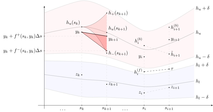 Figure 1
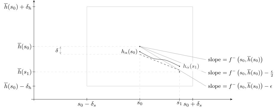 Figure 2
Peer Reviews
No public reviews on file for this paper yet. If you reviewed it on a platform where reviews are public (OpenReview, ICLR, NeurIPS, ICML), you can paste yours below so the community can read it here.
Videos
No videos yet. Explain this paper in a talk, walkthrough, or lecture? Add one.
Asymptotic Optimality of a Time Optimal
Path Parametrization Algorithm
Igor Spasojevic
Varun Murali
Sertac Karaman Laboratory of Information and Decision Systems, Massachusetts Institute of Technology, 32 Vassar Street. This work was partly supported by the Office of Naval Research (ONR) and the Army Research Lab DCIST project. {igorspas, mvarun, sertac}@mit.edu
Abstract
Time Optimal Path Parametrization is the problem of minimizing the time interval during which an actuation constrained agent can traverse a given path. Recently, an efficient linear-time algorithm for solving this problem was proposed [1]. However, its optimality was proved for only a strict subclass of problems solved optimally by more computationally intensive approaches based on convex programming. In this paper, we prove that the same linear-time algorithm is asymptotically optimal for all problems solved optimally by convex optimization approaches. We also characterize the optimum of the Time Optimal Path Parametrization Problem, which may be of independent interest.
I Introduction
Time optimal path parametrization is the problem of finding the shortest time required by a differentially constrained agent to execute a specified geometric path. For example, consider an autonomous race car that has to complete a given race track in minimum time. The path of the race car on the plane is fixed. Its speed along this path needs to be decided, given actuation constraints that, e.g., limit its acceleration.
Seminal work on time optimal path parametrization dealt with planning trajectories for robotic manipulators [2]. The first algorithm [2], enhanced thereafter in numerous works [3], was theoretically grounded on Pontryagin’s Maximum Principle [4]. This class of algorithms determined the optimal speed profile, a function mapping the position of the agent along the path to its speed, by stitching together integral curves arising from a bang-bang control policy. Although theoretically sound and computationally efficient, these algorithms were beset by issues of numerical instability [1].
More recent line of work [5] [6] built on the insight that a whole spectrum of time optimal path parametrization problems could be cast as a convex optimization problem after a suitable change of variables. These algorithms solve for the optimal squared speed profile. Under such reparametrization, typical constraints on velocity and acceleration of the agent, as well as the path traversal time, become convex functions of the decision variables. Specifically, convex optimization approaches first partition the path by a sequence of discretization points. They then jointly recover approximations of the optimal squared speed profile at every point [5] [6]. Although these methods are both numerically stable and converge to optimal solutions, their time complexity is considered to be high for many practical real-time robotics applications [1].
Similar to the convex-optimization-based approaches, algorithms developed in [1, 7, 8, 9] approximate the optimal squared speed at a set of discretization points. In addition to being numerically stable, they are computationally efficient [1], which they achieve by exploiting additional structure possessed by time optimal path parametrization problems. However, their optimality has been established for only a strict subset of problems solved optimally by convex optimization approaches [1].
This paper shows the algorithm outlined in [1] is in fact optimal in the limit as the distance between consecutive discretization points tends to zero. The main contribution of this paper is twofold. First, we develop a characterization of the optimal solution using results from non-smooth analysis [10] and non-linear control [11] that have not been previously used in this context to the best of our knowledge (Theorem 3). Second, we uncover a natural relationship between continuous solutions and those defined on a set of discretization points as output by all numerical algorithms (Theorem 5).
This paper is organized as follows. In section II, we present the necessary background on non-smooth analysis used for the problem definition presented in Section III. In Section IV, we present our first main result that characterizes the optimal solution. We recall the algorithm given in [1] in Section V, and we present our second main result that proves the asymptotic optimality of this algorithm in Section VI.
II Preliminaries on Non-Smooth Analysis
Definition 1
[11, 10]** For a continuous function , we define functions given by
[TABLE]
for all . Additionally, is called Dini differentiable if both and take on values strictly in .
By definition, for all . Furthermore, is right differentiable at if and only if , in which case its right derivative equals . For every pair of Dini differentiable functions and , non-negative , and right differentiable function :
2. 2.
3. 3.
4. 4.
5. 5.
.
The following theorem is one of the fundamental results of non-smooth analysis.
Theorem 1
[10]** Let be a continuous function. The following are equivalent:
* is monotonically decreasing on * 2. 2.
* for all * 3. 3.
* for all .*
Theorem 1 has two important corollaries. Firstly, Property (4) of Dini derivatives implies a continuous function is monotonically increasing if and only if and are non-negative functions. Second, if is bounded above (below) by , property 5 implies for all .
III Problem Definition
A concrete example of time optimal path parametrization involves minimizing the time a car requires to traverse a specified smooth geometric path . For the sake of simplicity, we assume is parametrized by arc length. Constraints consist of upper bounds on the magnitudes of velocity and acceleration of the car at every point along the path. Letting , we have [5, 6]:
[TABLE]
The bound on velocity is equivalent to , while the bound on acceleration translates into
[TABLE]
For the very simple case of moving optimally along a straight line segment after starting from rest, the acceleration of the car switches from to . At the switching point, the squared speed has discontinuous slope. To seamlessy deal with such behaviour, we drop the requirement that be a differentiable function and substitute Condition (1) by and for suitably chosen functions and . In the most general form, we solve problem :
[TABLE]
The former example is clearly a special case of the latter problem, as can be seen by setting , , , , and .
We note that if a pair of feasible solutions and satisfies for all , has a lower cost than .
IV Characterization of Optimum
The main result of this section is presented in Theorem 3. We prove that the function defined as the pointwise supremum of all functions that are feasible for problem is also feasible and therefore optimal (Theorem 3(a)). We use this characterization to show continuity of the optimum with respect to a natural parameter quantifying the degree of relaxation of constraints of (Theorem 3(b)). Finally, we prove that the feasible set of is convex (Theorem 3(c)). To begin with, we note a useful result from Lipschitz analysis.
Theorem 2
[12]** Let be an arbitrary non-empty family of uniformly bounded -Lipschitz functions defined on interval . Functions , defined by
[TABLE]
for all , are well-defined and -Lipschitz.
Theorem 3
Let be a pair of continuous functions with for all . Define region . Suppose are a pair of continuous functions with for all . In particular, for some . For a real number , a function is called -feasible if it satisfies the following conditions:
* is continuous* 2. 2.
* for all * 3. 3.
* for all * 4. 4.
* for all .*
Let denote the set of -feasible functions.
- a)
Assume for some (possibly uncountable) index set . Then, , defined by
[TABLE]
*for all , are -feasible functions. * 2. b)
Assume . Define . Then,
[TABLE] 3. c)
Assume functions and are concave and convex in their second arguments respectively. For every , for every pair of -feasible functions and , and for every , the function is also -feasible.
Proof.
(a) We only give detailed proof of the claim for and . The corresponding result for when can be recovered from the result for by redefining . Similarly, the result for can be recovered from the result for by redefining , , and using Properties - of Dini derivatives.
Since functions and are continuous on , they are bounded. As , is well defined. For arbitrary , taking the supremum over of the inequality , we verify satisfies Condition . In particular, and are defined at all points for .
The fact that implies is -Lipschitz for all . By Theorem 2, is also -Lipschitz; in particular is continuous, thus verifying Condition .
Next, we show satisfies Condition . Assume, for a contradiction, for some (see Figure 1). Hence, there exists such that .
Continuity of implies there exist such that for all . Keeping intact while shrinking if necessary, we may assume
[TABLE]
The definition of implies there exists a decreasing sequence tending to as and for all . In particular, we may assume satisfies
[TABLE]
Define
[TABLE]
The definition of implies there exists such that
[TABLE]
Since is -Lipschitz, it follows that for all we have
[TABLE]
Hence, for all
[TABLE]
implying
[TABLE]
By the second corollary to Theorem 1,
[TABLE]
where the last inequality follows from Equation (4). However, Equation (9) violates the definition of at . This gives the desired contradiction, and shows satisfies Condition (3). The proof that satisfies Condition (4) is ommitted since it can be derived analogously.
(b) Consider arbitrary real numbers . According to part (a) of Theorem 3, . This implies . Hence, for every , is monotonically increasing in and bounded below by . As a result, function , given by for all , is well defined and satisfies .
On the other hand, monotonicity of implies for every . Since for every , another application of part (a) of Theorem 3 to the non-empty set of functions yields . Since was arbitrary, we have . By definition of , we thus have .
Combining previous observations, we get . Thus, as for all . Since functions are continuous on interval , uniform convergence follows.
(c) Consider any and . Function clearly satisfies Conditions (1) and (2) of Theorem 3, so we turn to deriving Condition (3). As in part (a), the proof of Condition (4) is ommitted as it can be derived analogously. We have:
[TABLE]
The first inequality above follows from Properties () and () of Dini derivatives, whereas the second inequality follows from -feasibility of and . Finally, the last inequality follows from convexity of in its second argument. ∎
V Algorithm
In this section, we recall the algorithm presented in [1] for obtaining a numerical approximation to the optimal solution characterized in the previous section.
We first recall standard concepts from numerical analysis, which will be used for describing and analyzing the algorithm. A discretization of interval is an increasing sequence of points satisfying . We denote its cardinality by , and its resolution by .
Given a discretization and problem , a numerical procedure aims to find approximations to the optimal solution at points . Its error is defined as , and it is said to be asymptotically optimal if as .
Algorithm 1 is a recently-proposed algorithm for solving problem numerically. It incrementally constructs an approximation to the optimum in a pair of sweeps through . As a result, it has linear time-complexity in . This makes it orders of magnitude faster than approaches employing general purpose convex optimization libraries, whose time complexity is super-linear in [1]. However, despite its computational efficiency, Algorithm 1 had been proven to converge to optimal solutions for only a subclass of problems that can be optimally solved by convex programming in [5].
VI Asymptotic Optimality
The main result of this section is Theorem 5 which proves asymptotic optimality of Algorithm 1 for all feasible problems amenable to convex optimization approaches.
First, in Theorem 4 we recall an important result, which:
- a)
characterizes a lower bound on the length of the interval on which a solution to an ordinary differential equation is defined 2. b)
proves that a continuous function can never exceed a differentiable function whose derivative upper bounds the former’s Dini derivative.
Theorem 4
[11]** In addition to the setup of Theorem 3, let:
* and satisfy * 2. 2.
for every pair of continuous functions such that , there exist such that and are -Lipschitz and -Lipschitz on in their first and second arguments respectively.
Consider arbitrary , , and such that .
- a)
There exists such that the initial value problem
[TABLE]
admits a unique solution on interval . Furthermore, we may choose
[TABLE] 2. b)
Every continuous function , such that and for all , satisfies
[TABLE]
for all .
Before turning to the main result of the section, we give a definition. For a problem and discretization , we call a sequence admissible if for all , and for all . Additionally, we will denote by () the pointwise supremum (infimum) of all feasible functions for .
Theorem 5
Assume in addition to the setup of Theorem 4, problem is feasible and . For every , there exists an such that for every discretization with resolution , Algorithm 1 returns an admissible sequence with .
Proof.
Fix an arbitrary . The proof will consist of two parts. We will show there exist such that for every discretization with resolution at most (), Algorithm 1 produces an admissible sequence satisfying () for all . Clearly setting yields proof of the theorem.
To prove the first part, consider feasible functions and such that . Such functions exist by assumption and part (c) of Theorem 3. Define , , and . Clearly .
Set . By assumption, there exist such that for all we have
[TABLE]
Choose
[TABLE]
We claim that for any discretization with resolution , Algorithm 1 produces an admissible sequence satisfying for all .
The proof of the claim will proceed in two stages. The first will show the sequence generated by the backward pass satisfies for all . The second will show the sequence generated by the forward pass satisfies for all .
Lemma 1
There exist admissible sequences and such that for every , we have and (see Figure 2).
Proof.
We only prove existence of as that of follows analogously. To this end, define given by
[TABLE]
for all . Clearly . We will inductively construct an admissible sequence which satisfies , thus proving the lemma.
Set . Assume we have defined an admissible sequence satisfying for all . We now define .
By part (a) of Theorem 4, the choice of , along with boundedness and Lipschitz continuity of and on , implies existence and uniqueness of solutions to initial value problems
[TABLE]
on interval . Furthermore, part (b) of Theorem 4 implies for all . In particular, .
Define . Lipschitz continuity of and Equation (13) imply (see Figure 2)
[TABLE]
Similarly,
[TABLE]
Since an admissible value of can take on any value in the range , Equations (14) and (15) imply the existence of admissible satisfying
[TABLE]
where the second inequality follows from the inductive hypothesis, and the third from the definition of after a small amount of algebra. This completes proofs of the inductive step and the lemma.
∎
We now return to proofs of stages one and two. Assume sequences and have been constructed as in Lemma 1. Existence of immediately implies the sequence is well-defined and satisfies for all . This finishes the proof of stage one.
For stage two, we prove by induction on that is well-defined and satisfies for all . The base case follows from . For the inductive hypothesis, assume the statement holds for . We now show it also holds for . The definition of the backward pass implies there exists such that
[TABLE]
We recall assumption along with feasibility of implies is -Lipschitz. Thus,
[TABLE]
Since , we have
[TABLE]
Since (see Figure 2), there exists such that . Consider . Equation (19) implies
[TABLE]
Furthermore,
[TABLE]
where the first inequality above follows from Equation (17) and admissibility of , and the second inequality from convexity of in its second argument. Similarly, we obtain
[TABLE]
Equations (20), (21), and (22) imply is well-defined and satisfies . This finishes the proof of the inductive step, the proof of stage two and of the first part of the theorem.
To prove the second part, consider such that . Such exists due to part (b) of Theorem 3. Uniform continuity of implies there exists
[TABLE]
such that for all we have
[TABLE]
Uniform continuity of implies there exists
[TABLE]
such that for all we have
[TABLE]
Consider arbitrary discretization with . Let be the sequence output by Algorithm 1. Define function via for all , and
[TABLE]
for all and . By construction, is continuous. In fact, we show .
First we will prove . Consider any . Since is linear on , for all . Thus, it suffices to show . To this end, consider arbitrary . Since , Equation (26) implies . Admissibility of implies and so
[TABLE]
Since was arbitrary, we obtain . The correspnding inequality for follows analogously, and so holds.
Next, we show for all . Again, consider arbitrary and . We have
[TABLE]
Also,
[TABLE]
where the first equality follows from linearity of on , and the second inequality from admissibility of and the fact . Equations (24) and (30) imply . Similarly, implies . Combining the latter pair of inequalities, we derive . Similarly, , and so we obtain .
As a result, by definition of , we have . This implies for every
[TABLE]
where the last inequality follows from Equation (23). This finishes the proof of the theorem.
∎
VII Conclusion
This paper presented two main results. First, it characterized the optimum of a large class of problems in time optimal path parametrization. Second, it proved the asymptotic optimality of a recently-proposed algorithm for solving this class of problems with linear (optimal) time complexity. This result extends its asymptotic optimality guarantee to all problems that are solved by relatively computationally more demanding convex-optimization-based methods. Let us note that, although we focused on the analysis of the algorithm presented in [1], intermediate results in the proof of Theorem 5 could easily be combined to yield asymptotic optimality of the algorithm in [8].
The reference list from the paper itself. Each links out to its DOI / PubMed record.
- 1[1] H. Pham and Q. C. Pham, “A New Approach to Time-Optimal Path Parameterization Based on Reachability Analysis,” IEEE Transactions on Robotics , vol. 34, pp. 645 – 659, 06 2018.
- 2[2] J. Bobrow, S. Dubowsky, and J. S. Gibson, “Time-Optimal Control of Robotic Manipulators Along Specified Paths,” International Journal of Robotic Research - IJRR , vol. 4, pp. 3–17, 09 1985.
- 3[3] Q. C. Pham, “A General, Fast, and Robust Implementation of the Time-Optimal Path Parameterization Algorithm,” IEEE Transactions on Robotics , vol. 30, 12 2013.
- 4[4] L. S. Pontryagin, The Mathematical Theory of Optimal Processes . CRC Press, 03 1987.
- 5[5] T. Lipp and S. Boyd, “Minimum-time speed optimisation over a fixed path,” International Journal of Control , vol. 87, 02 2014.
- 6[6] D. Verscheure, B. Demeulenaere, J. Swevers, J. De Schutter, and M. Diehl, “Time-Optimal Path Tracking for Robots: A Convex Optimization Approach,” Automatic Control, IEEE Transactions on , vol. 54, pp. 2318 – 2327, 11 2009.
- 7[7] L. Consolini, M. Locatelli, A. Minari, and A. Piazzi, “An optimal complexity algorithm for minimum-time velocity planning,” Systems & Control Letters , vol. 103, pp. 50–57, 05 2017.
- 8[8] G. Csorvási, A. Nagy, and I. Vajk, “Near time-optimal path tracking method for waiter motion problem,” vol. 50, 07 2017, pp. 4929–4934.