The Event Horizon General Relativistic Magnetohydrodynamic Code Comparison Project
Oliver Porth, Koushik Chatterjee, Ramesh Narayan, Charles F. Gammie,, Yosuke Mizuno, Peter Anninos, John G. Baker, Matteo Bugli, Chi-kwan Chan,, Jordy Davelaar, Luca Del Zanna, Zachariah B. Etienne, P. Chris Fragile,, Bernard J. Kelly, Matthew Liska, Sera Markoff

TL;DR
This paper compares nine general relativistic magnetohydrodynamics (GRMHD) codes on a common accretion flow problem, demonstrating their maturity, consistency, and improved agreement with higher resolution.
Contribution
It provides a comprehensive comparison of nine GRMHD codes, establishing their reliability and consistency for modeling astrophysical phenomena near compact objects.
Findings
Code agreement improves with resolution
Community of GRMHD codes is mature and capable
Codes produce consistent results on test problems
Abstract
Recent developments in compact object astrophysics, especially the discovery of merging neutron stars by LIGO, the imaging of the black hole in M87 by the Event Horizon Telescope (EHT) and high precision astrometry of the Galactic Center at close to the event horizon scale by the GRAVITY experiment motivate the development of numerical source models that solve the equations of general relativistic magnetohydrodynamics (GRMHD). Here we compare GRMHD solutions for the evolution of a magnetized accretion flow where turbulence is promoted by the magnetorotational instability from a set of nine GRMHD codes: Athena++, BHAC, Cosmos++, ECHO, H-AMR, iharm3D, HARM-Noble, IllinoisGRMHD and KORAL. Agreement between the codes improves as resolution increases, as measured by a consistently applied, specially developed set of code performance metrics. We conclude that the community of GRMHD codes is…
Click any figure to enlarge with its caption.
 Figure 1
 Figure 2
 Figure 3
 Figure 4
 Figure 5
 Figure 6
 Figure 7
 Figure 8
 Figure 9
 Figure 10
 Figure 11
 Figure 12
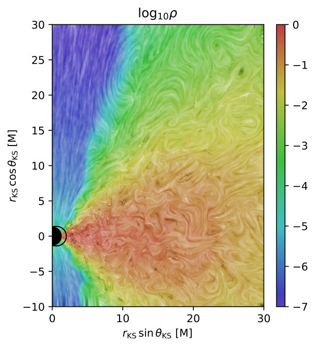 Figure 13
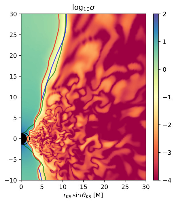 Figure 14
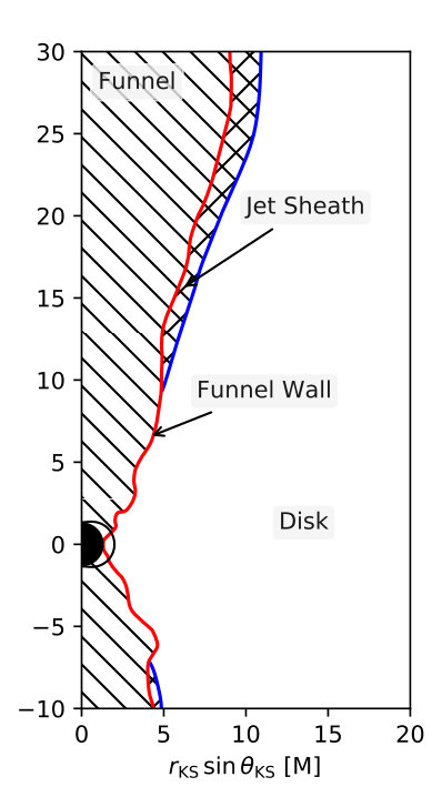 Figure 15
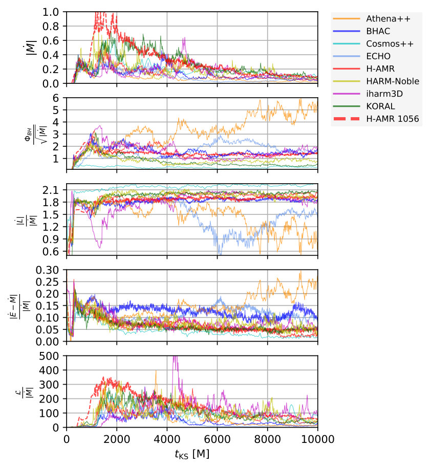 Figure 16
 Figure 17
 Figure 18
 Figure 19
 Figure 20
 Figure 21
 Figure 22
 Figure 23
 Figure 24
 Figure 25
 Figure 26
 Figure 27
 Figure 28
 Figure 29
 Figure 30
 Figure 31
 Figure 32
 Figure 33
 Figure 34
 Figure 35
| Code | Timestepper | Riemann s. | Rec. | Mag. field | Domain: r | Domain: | |
| Athena++ | 2nd Order | HLL | PPM | CT (Gardiner & Stone, 2005) | |||
| BHAC | 2nd Order | LLF | PPM | UCT (Del Zanna et al., 2007) | |||
| BHAC Cart. | 2nd Order | LLF | PPM | UCT (Del Zanna et al., 2007) | Cartesian AMR | See Sect. 4.1.2. | – |
| Cosmos++ | SSPRK, 3rd Order | HLL | PPM | (Fragile et al., 2012) | |||
| ECHO | 3rd Order | HLL | PPM | UCT (Del Zanna et al., 2007) | |||
| H-AMR | 2nd Order | HLL | PPM | UCT (Gardiner & Stone, 2005) | |||
| HARM-Noble | 2nd Order | LLF | PPM | PPM+Flux-CT (Tóth, 2000), (Noble et al., 2009) | |||
| iharm3D | 2nd Order | LLF | PLM | Flux-CT (Tóth, 2000) | |||
| IllinoisGRMHD | RK4 | HLL | PPM | Vector potential-based PPM+Flux-CT (Tóth, 2000), (Etienne et al., 2010), (Etienne et al., 2012b) | Cartesian AMR | See Sect. 4.1.8. | – |
| KORAL | 2nd order | LLF | PPM | Flux-CT (Tóth, 2000) |
| Code | |||||||||
| 96 | Athena++ | ||||||||
| BHAC | |||||||||
| Cosmos++ | |||||||||
| ECHO | |||||||||
| H-AMR | |||||||||
| HARM-Noble | |||||||||
| iharm3D | |||||||||
| KORAL | |||||||||
| max/min | 2.406 | 3.903 | 12.374 | 17.408 | 1.163 | 1.823 | 1.448 | 7.096 | |
| 128 | Athena++ | ||||||||
| BHAC | |||||||||
| BHAC Cart. | |||||||||
| Cosmos++ | |||||||||
| ECHO | |||||||||
| H-AMR | |||||||||
| HARM-Noble | |||||||||
| iharm3D | |||||||||
| IllinoisGRMHD | |||||||||
| KORAL | |||||||||
| max/min | 2.525 | 8.604 | 11.126 | 12.24 | 1.16 | 1.201 | 1.552 | 4.631 | |
| 192 | Athena++ | ||||||||
| BHAC | |||||||||
| ECHO | |||||||||
| H-AMR | |||||||||
| HARM-Noble | |||||||||
| iharm3D | |||||||||
| KORAL | |||||||||
| max/min | 1.649 | 1.772 | 2.116 | 2.777 | 1.077 | 1.121 | 1.25 | 1.405 | |
| BHAC | |||||||||
| 384 | BHAC | ||||||||
| 1056 | H-AMR |
| Code | |||||||||
| 96 | Athena++ | ||||||||
| H-AMR | |||||||||
| KORAL | |||||||||
| max/min | 4.296 | 2.062 | 3.913 | 3.62 | 1.112 | 1.177 | 1.358 | 7.258 | |
| 128 | Athena++ | ||||||||
| H-AMR | |||||||||
| KORAL | |||||||||
| max/min | 2.665 | 5.165 | 5.41 | 5.439 | 1.177 | 1.527 | 1.117 | 4.049 | |
| 192 | Athena++ | ||||||||
| H-AMR | |||||||||
| KORAL | |||||||||
| max/min | 1.88 | 5.027 | 2.489 | 2.23 | 1.031 | 1.362 | 1.016 | 2.967 |
| Code | |||||||||
| 96 | KORAL Odyssey | ||||||||
| KORAL Stampede2 | |||||||||
| max/min | 1.106 | 1.024 | 1.075 | 1.349 | 1.01 | 1.008 | 1.0 | 1.009 | |
| 128 | KORAL Odyssey | ||||||||
| KORAL Stampede2 | |||||||||
| max/min | 1.417 | 1.134 | 1.031 | 1.093 | 1.011 | 1.008 | 1.0 | 1.053 | |
| 192 | KORAL Odyssey | ||||||||
| KORAL Stampede2 | |||||||||
| max/min | 1.144 | 1.128 | 1.049 | 1.237 | 1.006 | 1.014 | 1.0 | 1.014 |
Peer Reviews
No public reviews on file for this paper yet. If you reviewed it on a platform where reviews are public (OpenReview, ICLR, NeurIPS, ICML), you can paste yours below so the community can read it here.
Videos
No videos yet. Explain this paper in a talk, walkthrough, or lecture? Add one.
The Event Horizon General Relativistic Magnetohydrodynamic Code Comparison Project
Anton Pannekoek Institute for Astronomy, University of Amsterdam, Science Park 904, 1098 XH, Amsterdam, The Netherlands
Institut für Theoretische Physik, Goethe-Universität Frankfurt, Max-von-Laue-Straße 1, D-60438 Frankfurt am Main, Germany
Koushik Chatterjee
Anton Pannekoek Institute for Astronomy, University of Amsterdam, Science Park 904, 1098 XH, Amsterdam, The Netherlands
Center for Astrophysics Harvard & Smithsonian, 60 Garden Street, Cambridge, MA 02138, USA
Black Hole Initiative at Harvard University, 20 Garden Street, Cambridge, MA 02138, USA
Department of Astronomy; Department of Physics; University of Illinois, Urbana, IL 61801 USA
Institut für Theoretische Physik, Goethe-Universität Frankfurt, Max-von-Laue-Straße 1, D-60438 Frankfurt am Main, Germany
Peter Anninos
Lawrence Livermore National Laboratory, Livermore, CA 94550, USA
John G. Baker
Gravitational Astrophysics Laboratory, NASA Goddard Space Flight Center, Greenbelt, MD 20771, USA
Joint Space-Science Institute, University of Maryland, College Park, MD 20742, USA
IRFU/Département d’Astrophysique, Laboratoire AIM, CEA/DRF-CNRS-Université Paris Diderot, CEA-Saclay F-91191, France
Steward Observatory and Department of Astronomy, University of Arizona, 933 N. Cherry Ave., Tucson, AZ 85721, USA
Data Science Institute, University of Arizona, 1230 N. Cherry Ave., Tucson, AZ 85721, USA
Department of Astrophysics, Institute for Mathematics, Astrophysics and Particle Physics (IMAPP), Radboud University, P.O. Box 9010, 6500 GL Nijmegen, The Netherlands
Luca Del Zanna
Dipartimento di Fisica e Astronomia, Università di Firenze e INFN – Sez. di Firenze, via G. Sansone 1, I-50019 Sesto F.no, Italy
INAF, Osservatorio Astrofisico di Arcetri, Largo E. Fermi 5, I-50125 Firenze, Italy
Zachariah B. Etienne
Department of Mathematics, West Virginia University, Morgantown, WV 26506, USA
Center for Gravitational Waves and Cosmology, West Virginia University, Chestnut Ridge Research Building, Morgantown, WV 26505, USA
P. Chris Fragile
Department of Physics & Astronomy, College of Charleston, 66 George St., Charleston, SC 29424, USA
Department of Physics, University of Maryland, Baltimore County, Baltimore, MD 21250, USA
CRESST, NASA Goddard Space Flight Center, Greenbelt, MD 20771, USA
Gravitational Astrophysics Laboratory, NASA Goddard Space Flight Center, Greenbelt, MD 20771, USA
Matthew Liska
Anton Pannekoek Institute for Astronomy, University of Amsterdam, Science Park 904, 1098 XH, Amsterdam, The Netherlands
Sera Markoff
Anton Pannekoek Institute for Astronomy & GRAPPA, University of Amsterdam, Postbus 94249, 1090GE Amsterdam, The Netherlands
Jonathan C. McKinney
H2O.ai, 2307 Leghorn St., Mountain View, CA 94043
Bhupendra Mishra
JILA, University of Colorado and National Institute of Standards and Technology, 440 UCB, Boulder, CO 80309-0440, USA
Department of Physics and Engineering Physics, The University of Tulsa, Tulsa, OK 74104, USA
Gravitational Astrophysics Laboratory, NASA Goddard Space Flight Center, Greenbelt, MD 20771, USA
Institut für Theoretische Physik, Goethe-Universität Frankfurt, Max-von-Laue-Straße 1, D-60438 Frankfurt am Main, Germany
Department of Physics, University of Illinois, 1110 West Green St, Urbana, IL 61801, USA
Luciano Rezzolla
Institut für Theoretische Physik, Goethe-Universität Frankfurt, Max-von-Laue-Straße 1, D-60438 Frankfurt am Main, Germany
CCS-2, Los Alamos National Laboratory, P.O. Box 1663, Los Alamos, NM 87545, US
Center for Theoretical Astrophysics, Los Alamos National Laboratory, Los Alamos, NM, 87545, USA
James M. Stone
Department of Astrophysical Sciences, Princeton University, Princeton, NJ 08544, USA
Niccolò Tomei
Dipartimento di Fisica e Astronomia, Università di Firenze e INFN – Sez. di Firenze, via G. Sansone 1, I-50019 Sesto F.no, Italy
INAF, Osservatorio Astrofisico di Arcetri, Largo E. Fermi 5, I-50125 Firenze, Italy
Christopher J. White
Kavli Institute for Theoretical Physics, University of California Santa Barbara, Kohn Hall, Santa Barbara, CA 93107, USA
Mullard Space Science Laboratory, University College London, Holmbury St. Mary, Dorking, Surrey, RH5 6NT, United Kingdom
Institut für Theoretische Physik, Goethe-Universität Frankfurt, Max-von-Laue-Straße 1, D-60438 Frankfurt am Main, Germany
National Radio Astronomy Observatory, 520 Edgemont Rd, Charlottesville, VA 22903, USA
Massachusetts Institute of Technology Haystack Observatory, 99 Millstone Road, Westford, MA 01886, USA
National Astronomical Observatory of Japan, 2-21-1 Osawa, Mitaka, Tokyo 181-8588, Japan
Black Hole Initiative at Harvard University, 20 Garden Street, Cambridge, MA 02138, USA
Instituto de Astrofísica de Andalucía - CSIC, Glorieta de la Astronomía s/n, E-18008 Granada, Spain
Walter Alef
Max-Planck-Institut für Radioastronomie, Auf dem Hügel 69, D-53121 Bonn, Germany
Keiichi Asada
Institute of Astronomy and Astrophysics, Academia Sinica, 11F of Astronomy-Mathematics Building, AS/NTU No. 1, Sec. 4, Roosevelt Rd, Taipei 10617, Taiwan, R.O.C.
Departament d’Astronomia i Astrofísica, Universitat de València, C. Dr. Moliner 50, E-46100 Burjassot, València, Spain
Observatori Astronòmic, Universitat de València, C. Catedrático José Beltrán 2, E-46980 Paterna, València, Spain
Max-Planck-Institut für Radioastronomie, Auf dem Hügel 69, D-53121 Bonn, Germany
Max-Planck-Institut für Radioastronomie, Auf dem Hügel 69, D-53121 Bonn, Germany
David Ball
Steward Observatory and Department of Astronomy, University of Arizona, 933 N. Cherry Ave., Tucson, AZ 85721, USA
Center for Astrophysics Harvard & Smithsonian, 60 Garden Street, Cambridge, MA 02138, USA
Black Hole Initiative at Harvard University, 20 Garden Street, Cambridge, MA 02138, USA
Massachusetts Institute of Technology Haystack Observatory, 99 Millstone Road, Westford, MA 01886, USA
Dan Bintley
East Asian Observatory, 660 N. A’ohoku Pl., Hilo, HI 96720, USA
Center for Astrophysics Harvard & Smithsonian, 60 Garden Street, Cambridge, MA 02138, USA
Black Hole Initiative at Harvard University, 20 Garden Street, Cambridge, MA 02138, USA
Wilfred Boland
Nederlandse Onderzoekschool voor Astronomie (NOVA), PO Box 9513, 2300 RA Leiden, the Netherlands, Niels Bohrweg 2, 2333 CA Leiden, the Netherlands
Center for Astrophysics Harvard & Smithsonian, 60 Garden Street, Cambridge, MA 02138, USA
Black Hole Initiative at Harvard University, 20 Garden Street, Cambridge, MA 02138, USA
California Institute of Technology, 1200 East California Boulevard, Pasadena, CA 91125, USA
Institute of Astronomy and Astrophysics, Academia Sinica, 645 N. A’ohoku Place, Hilo, HI 96720, USA
Michael Bremer
Institut de Radioastronomie Millimétrique, 300 rue de la Piscine, 38406 Saint Martin d’Hères, France
Department of Astrophysics, Institute for Mathematics, Astrophysics and Particle Physics (IMAPP), Radboud University, P.O. Box 9010, 6500 GL Nijmegen, The Netherlands
Center for Astrophysics Harvard & Smithsonian, 60 Garden Street, Cambridge, MA 02138, USA
Black Hole Initiative at Harvard University, 20 Garden Street, Cambridge, MA 02138, USA
Max-Planck-Institut für Radioastronomie, Auf dem Hügel 69, D-53121 Bonn, Germany
Perimeter Institute for Theoretical Physics, 31 Caroline Street North, Waterloo, ON, N2L 2Y5, Canada
Department of Physics and Astronomy, University of Waterloo, 200 University Avenue West, Waterloo, ON, N2L 3G1, Canada
Waterloo Centre for Astrophysics, University of Waterloo, Waterloo, ON N2L 3G1 Canada
Dominique Broguiere
Institut de Radioastronomie Millimétrique, 300 rue de la Piscine, 38406 Saint Martin d’Hères, France
Thomas Bronzwaer
Department of Astrophysics, Institute for Mathematics, Astrophysics and Particle Physics (IMAPP), Radboud University, P.O. Box 9010, 6500 GL Nijmegen, The Netherlands
Korea Astronomy and Space Science Institute, Daedeok-daero 776, Yuseong-gu, Daejeon 34055, Republic of Korea
University of Science and Technology, Gajeong-ro 217, Yuseong-gu, Daejeon 34113, Republic of Korea
John E. Carlstrom
Kavli Institute for Cosmological Physics, University of Chicago, Chicago, IL 60637, USA
Department of Astronomy and Astrophysics, University of Chicago, Chicago, IL 60637, USA
Department of Physics, University of Chicago, Chicago, IL 60637, USA
Enrico Fermi Institute, University of Chicago, Chicago, IL 60637, USA
Center for Astrophysics Harvard & Smithsonian, 60 Garden Street, Cambridge, MA 02138, USA
Black Hole Initiative at Harvard University, 20 Garden Street, Cambridge, MA 02138, USA
Cornell Center for Astrophysics and Planetary Science, Cornell University, Ithaca, NY 14853, USA
Ming-Tang Chen
Institute of Astronomy and Astrophysics, Academia Sinica, 645 N. A’ohoku Place, Hilo, HI 96720, USA
Yongjun Chen (陈永军)
Shanghai Astronomical Observatory, Chinese Academy of Sciences, 80 Nandan Road, Shanghai 200030, China
Key Laboratory of Radio Astronomy, Chinese Academy of Sciences, Nanjing 210008, China
Korea Astronomy and Space Science Institute, Daedeok-daero 776, Yuseong-gu, Daejeon 34055, Republic of Korea
University of Science and Technology, Gajeong-ro 217, Yuseong-gu, Daejeon 34113, Republic of Korea
Steward Observatory and Department of Astronomy, University of Arizona, 933 N. Cherry Ave., Tucson, AZ 85721, USA
Center for Astrophysics Harvard & Smithsonian, 60 Garden Street, Cambridge, MA 02138, USA
Department of Space, Earth and Environment, Chalmers University of Technology, Onsala Space Observatory, SE-439 92 Onsala, Sweden
Cornell Center for Astrophysics and Planetary Science, Cornell University, Ithaca, NY 14853, USA
Massachusetts Institute of Technology Haystack Observatory, 99 Millstone Road, Westford, MA 01886, USA
Mizusawa VLBI Observatory, National Astronomical Observatory of Japan, 2-12 Hoshigaoka, Mizusawa, Oshu, Iwate 023-0861, Japan
Department of Astronomical Science, The Graduate University for Advanced Studies (SOKENDAI), 2-21-1 Osawa, Mitaka, Tokyo 181-8588, Japan
Dipartimento di Fisica ”E. Pancini”, Universitá di Napoli ”Federico II”, Compl. Univ. di Monte S. Angelo, Edificio G, Via Cinthia, I-80126, Napoli, Italy
Institut für Theoretische Physik, Goethe-Universität Frankfurt, Max-von-Laue-Straße 1, D-60438 Frankfurt am Main, Germany
INFN Sez. di Napoli, Compl. Univ. di Monte S. Angelo, Edificio G, Via Cinthia, I-80126, Napoli, Italy
Department of Physics, University of Pretoria, Lynnwood Road, Hatfield, Pretoria 0083, South Africa; Centre for Radio Astronomy Techniques and Technologies, Department of Physics and Electronics, Rhodes University, Grahamstown 6140, South Africa
East Asian Observatory, 660 N. A’ohoku Pl., Hilo, HI 96720, USA
Max-Planck-Institut für Radioastronomie, Auf dem Hügel 69, D-53121 Bonn, Germany
Center for Astrophysics Harvard & Smithsonian, 60 Garden Street, Cambridge, MA 02138, USA
Black Hole Initiative at Harvard University, 20 Garden Street, Cambridge, MA 02138, USA
Max-Planck-Institut für Radioastronomie, Auf dem Hügel 69, D-53121 Bonn, Germany
Department of Astrophysics, Institute for Mathematics, Astrophysics and Particle Physics (IMAPP), Radboud University, P.O. Box 9010, 6500 GL Nijmegen, The Netherlands
Massachusetts Institute of Technology Haystack Observatory, 99 Millstone Road, Westford, MA 01886, USA
Ed Fomalont
National Radio Astronomy Observatory, 520 Edgemont Rd, Charlottesville, VA 22903, USA
Department of Astrophysics, Institute for Mathematics, Astrophysics and Particle Physics (IMAPP), Radboud University, P.O. Box 9010, 6500 GL Nijmegen, The Netherlands
Bill Freeman
Department of Electrical Engineering and Computer Science, Massachusetts Institute of Technology, 32-D476, 77 Massachussetts Ave., Cambridge, MA 02142, USA
Google Research, 355 Main St., Cambridge, MA 02142, USA
Per Friberg
East Asian Observatory, 660 N. A’ohoku Pl., Hilo, HI 96720, USA
Christian M. Fromm
Institut für Theoretische Physik, Goethe-Universität Frankfurt, Max-von-Laue-Straße 1, D-60438 Frankfurt am Main, Germany
Instituto de Astrofísica de Andalucía - CSIC, Glorieta de la Astronomía s/n, E-18008 Granada, Spain
Department of History of Science, Harvard University, Cambridge, MA 02138, USA
Department of Physics, Harvard University, Cambridge, MA 02138, USA
Black Hole Initiative at Harvard University, 20 Garden Street, Cambridge, MA 02138, USA
Roberto García
Institut de Radioastronomie Millimétrique, 300 rue de la Piscine, 38406 Saint Martin d’Hères, France
Olivier Gentaz
Institut de Radioastronomie Millimétrique, 300 rue de la Piscine, 38406 Saint Martin d’Hères, France
Department of Physics and Astronomy, University of Waterloo, 200 University Avenue West, Waterloo, ON, N2L 3G1, Canada
Ciriaco Goddi
Department of Astrophysics, Institute for Mathematics, Astrophysics and Particle Physics (IMAPP), Radboud University, P.O. Box 9010, 6500 GL Nijmegen, The Netherlands
Leiden Observatory - Allegro, Leiden University, P.O. Box 9513, 2300 RA Leiden, The Netherlands
Institut für Theoretische Physik, Goethe-Universität Frankfurt, Max-von-Laue-Straße 1, D-60438 Frankfurt am Main, Germany
Shanghai Astronomical Observatory, Chinese Academy of Sciences, 80 Nandan Road, Shanghai 200030, China
Key Laboratory for Research in Galaxies and Cosmology, Chinese Academy of Sciences, Shanghai 200030, China
Center for Astrophysics Harvard & Smithsonian, 60 Garden Street, Cambridge, MA 02138, USA
Mizusawa VLBI Observatory, National Astronomical Observatory of Japan, 2-12 Hoshigaoka, Mizusawa, Oshu, Iwate 023-0861, Japan
Department of Astronomical Science, The Graduate University for Advanced Studies (SOKENDAI), 2-21-1 Osawa, Mitaka, Tokyo 181-8588, Japan
Michael H. Hecht
Massachusetts Institute of Technology Haystack Observatory, 99 Millstone Road, Westford, MA 01886, USA
NOVA Sub-mm Instrumentation Group, Kapteyn Astronomical Institute, University of Groningen, Landleven 12, 9747 AD Groningen, The Netherlands
Department of Astronomy, School of Physics, Peking University, Beijing 100871, China
Kavli Institute for Astronomy and Astrophysics, Peking University, Beijing 100871, China
Paul Ho
Institute of Astronomy and Astrophysics, Academia Sinica, 11F of Astronomy-Mathematics Building, AS/NTU No. 1, Sec. 4, Roosevelt Rd, Taipei 10617, Taiwan, R.O.C.
Mizusawa VLBI Observatory, National Astronomical Observatory of Japan, 2-12 Hoshigaoka, Mizusawa, Oshu, Iwate 023-0861, Japan
Department of Astronomical Science, The Graduate University for Advanced Studies (SOKENDAI), 2-21-1 Osawa, Mitaka, Tokyo 181-8588, Japan
Institute of Astronomy and Astrophysics, Academia Sinica, 11F of Astronomy-Mathematics Building, AS/NTU No. 1, Sec. 4, Roosevelt Rd, Taipei 10617, Taiwan, R.O.C.
Lei Huang (黄磊)
Shanghai Astronomical Observatory, Chinese Academy of Sciences, 80 Nandan Road, Shanghai 200030, China
Key Laboratory for Research in Galaxies and Cosmology, Chinese Academy of Sciences, Shanghai 200030, China
David H. Hughes
Instituto Nacional de Astrofísica, Óptica y Electrónica. Apartado Postal 51 y 216, 72000. Puebla Pue., México
The Institute of Statistical Mathematics, 10-3 Midori-cho, Tachikawa, Tokyo, 190-8562, Japan
National Astronomical Observatory of Japan, 2-21-1 Osawa, Mitaka, Tokyo 181-8588, Japan
Department of Statistical Science, The Graduate University for Advanced Studies (SOKENDAI), 10-3 Midori-cho, Tachikawa, Tokyo 190-8562, Japan
Kavli Institute for the Physics and Mathematics of the Universe, The University of Tokyo, 5-1-5 Kashiwanoha, Kashiwa, 277-8583, Japan
Makoto Inoue
Institute of Astronomy and Astrophysics, Academia Sinica, 11F of Astronomy-Mathematics Building, AS/NTU No. 1, Sec. 4, Roosevelt Rd, Taipei 10617, Taiwan, R.O.C.
Department of Astrophysics, Institute for Mathematics, Astrophysics and Particle Physics (IMAPP), Radboud University, P.O. Box 9010, 6500 GL Nijmegen, The Netherlands
Center for Astrophysics Harvard & Smithsonian, 60 Garden Street, Cambridge, MA 02138, USA
Black Hole Initiative at Harvard University, 20 Garden Street, Cambridge, MA 02138, USA
Buell T. Jannuzi
Steward Observatory and Department of Astronomy, University of Arizona, 933 N. Cherry Ave., Tucson, AZ 85721, USA
Department of Astrophysics, Institute for Mathematics, Astrophysics and Particle Physics (IMAPP), Radboud University, P.O. Box 9010, 6500 GL Nijmegen, The Netherlands
Department of Physics and Astronomy, University of Waterloo, 200 University Avenue West, Waterloo, ON, N2L 3G1, Canada
Shanghai Astronomical Observatory, Chinese Academy of Sciences, 80 Nandan Road, Shanghai 200030, China
Center for Astrophysics Harvard & Smithsonian, 60 Garden Street, Cambridge, MA 02138, USA
Black Hole Initiative at Harvard University, 20 Garden Street, Cambridge, MA 02138, USA
Institute for Astrophysical Research, Boston University, 725 Commonwealth Ave., Boston, MA 02215
Astronomical Institute, St.Petersburg University, Universitetskij pr., 28, Petrodvorets,198504 St.Petersburg, Russia
Korea Astronomy and Space Science Institute, Daedeok-daero 776, Yuseong-gu, Daejeon 34055, Republic of Korea
University of Science and Technology, Gajeong-ro 217, Yuseong-gu, Daejeon 34113, Republic of Korea
Perimeter Institute for Theoretical Physics, 31 Caroline Street North, Waterloo, Ontario N2L 2Y5, Canada
University of Waterloo, 200 University Avenue West, Waterloo, Ontario N2L 3G1, Canada
Max-Planck-Institut für Radioastronomie, Auf dem Hügel 69, D-53121 Bonn, Germany
National Astronomical Observatory of Japan, 2-21-1 Osawa, Mitaka, Tokyo 181-8588, Japan
Center for Astrophysics Harvard & Smithsonian, 60 Garden Street, Cambridge, MA 02138, USA
Joint Institute for VLBI ERIC (JIVE), Oude Hoogeveensedijk 4, 7991 PD Dwingeloo, The Netherlands
Max-Planck-Institut für Radioastronomie, Auf dem Hügel 69, D-53121 Bonn, Germany
Steward Observatory and Department of Astronomy, University of Arizona, 933 N. Cherry Ave., Tucson, AZ 85721, USA
Jongsoo Kim
Korea Astronomy and Space Science Institute, Daedeok-daero 776, Yuseong-gu, Daejeon 34055, Republic of Korea
National Astronomical Observatory of Japan, 2-21-1 Osawa, Mitaka, Tokyo 181-8588, Japan
Kogakuin University of Technology & Engineering, Academic Support Center, 2665-1 Nakano, Hachioji, Tokyo 192-0015, Japan
Institute of Astronomy and Astrophysics, Academia Sinica, 11F of Astronomy-Mathematics Building, AS/NTU No. 1, Sec. 4, Roosevelt Rd, Taipei 10617, Taiwan, R.O.C.
Institute of Astronomy and Astrophysics, Academia Sinica, 11F of Astronomy-Mathematics Building, AS/NTU No. 1, Sec. 4, Roosevelt Rd, Taipei 10617, Taiwan, R.O.C.
Institute of Astronomy and Astrophysics, Academia Sinica, 11F of Astronomy-Mathematics Building, AS/NTU No. 1, Sec. 4, Roosevelt Rd, Taipei 10617, Taiwan, R.O.C.
Max-Planck-Institut für Radioastronomie, Auf dem Hügel 69, D-53121 Bonn, Germany
Institut de Radioastronomie Millimétrique, 300 rue de la Piscine, 38406 Saint Martin d’Hères, France
Max-Planck-Institut für Radioastronomie, Auf dem Hügel 69, D-53121 Bonn, Germany
Cheng-Yu Kuo
Physics Department, National Sun Yat-Sen University, No. 70, Lien-Hai Rd, Kaosiung City 80424, Taiwan, R.O.C
National Optical Astronomy Observatory, 950 North Cherry Ave., Tucson, AZ 85719, USA
Korea Astronomy and Space Science Institute, Daedeok-daero 776, Yuseong-gu, Daejeon 34055, Republic of Korea
Key Laboratory for Particle Astrophysics, Institute of High Energy Physics, Chinese Academy of Sciences, 19B Yuquan Road, Shijingshan District, Beijing, China
School of Astronomy and Space Science, Nanjing University, Nanjing 210023, China
Key Laboratory of Modern Astronomy and Astrophysics, Nanjing University, Nanjing 210023, China
Michael Lindqvist
Department of Space, Earth and Environment, Chalmers University of Technology, Onsala Space Observatory, SE-439 92 Onsala, Sweden
Max-Planck-Institut für Radioastronomie, Auf dem Hügel 69, D-53121 Bonn, Germany
Italian ALMA Regional Centre, INAF-Istituto di Radioastronomia, Via P. Gobetti 101, 40129 Bologna, Italy
Wen-Ping Lo
Department of Physics, National Taiwan University, No.1, Sect.4, Roosevelt Rd., Taipei 10617, Taiwan, R.O.C
Institute of Astronomy and Astrophysics, Academia Sinica, 11F of Astronomy-Mathematics Building, AS/NTU No. 1, Sec. 4, Roosevelt Rd, Taipei 10617, Taiwan, R.O.C.
Andrei P. Lobanov
Max-Planck-Institut für Radioastronomie, Auf dem Hügel 69, D-53121 Bonn, Germany
Instituto de Radioastronomía y Astrofísica, Universidad Nacional Autónoma de México, Morelia 58089, México
Instituto de Astronom\́Ia, Universidad Nacional Autónoma de México, CdMx 04510, México
Colin Lonsdale
Massachusetts Institute of Technology Haystack Observatory, 99 Millstone Road, Westford, MA 01886, USA
Shanghai Astronomical Observatory, Chinese Academy of Sciences, 80 Nandan Road, Shanghai 200030, China
Max-Planck-Institut für Radioastronomie, Auf dem Hügel 69, D-53121 Bonn, Germany
Max-Planck-Institut für Radioastronomie, Auf dem Hügel 69, D-53121 Bonn, Germany
Yunnan Observatories, Chinese Academy of Sciences, 650011 Kunming, Yunnan Province, China
Center for Astronomical Mega-Science, Chinese Academy of Sciences, 20A Datun Road, Chaoyang District, Beijing, 100012, China
Key Laboratory for the Structure and Evolution of Celestial Objects, Chinese Academy of Sciences, 650011 Kunming, China
Steward Observatory and Department of Astronomy, University of Arizona, 933 N. Cherry Ave., Tucson, AZ 85721, USA
Institute for Astrophysical Research, Boston University, 725 Commonwealth Ave., Boston, MA 02215, USA
Department of Space, Earth and Environment, Chalmers University of Technology, Onsala Space Observatory, SE-439 92 Onsala, Sweden
Centro Astronómico de Yebes (IGN), Apartado 148, 19180 Yebes, Spain
Satoki Matsushita
Institute of Astronomy and Astrophysics, Academia Sinica, 11F of Astronomy-Mathematics Building, AS/NTU No. 1, Sec. 4, Roosevelt Rd, Taipei 10617, Taiwan, R.O.C.
Massachusetts Institute of Technology Haystack Observatory, 99 Millstone Road, Westford, MA 01886, USA
Steward Observatory and Department of Astronomy, University of Arizona, 933 N. Cherry Ave., Tucson, AZ 85721, USA
Department of Physics, Broida Hall, University of California Santa Barbara, Santa Barbara, CA 93106, USA
Max-Planck-Institut für Radioastronomie, Auf dem Hügel 69, D-53121 Bonn, Germany
East Asian Observatory, 660 N. A’ohoku Pl., Hilo, HI 96720, USA
Center for Astrophysics Harvard & Smithsonian, 60 Garden Street, Cambridge, MA 02138, USA
Black Hole Initiative at Harvard University, 20 Garden Street, Cambridge, MA 02138, USA
Mizusawa VLBI Observatory, National Astronomical Observatory of Japan, 2-12 Hoshigaoka, Mizusawa, Oshu, Iwate 023-0861, Japan
Department of Astrophysics, Institute for Mathematics, Astrophysics and Particle Physics (IMAPP), Radboud University, P.O. Box 9010, 6500 GL Nijmegen, The Netherlands
Department of Astrophysics, Institute for Mathematics, Astrophysics and Particle Physics (IMAPP), Radboud University, P.O. Box 9010, 6500 GL Nijmegen, The Netherlands
Max-Planck-Institut für Radioastronomie, Auf dem Hügel 69, D-53121 Bonn, Germany
National Astronomical Observatory of Japan, Osawa 2-21-1, Mitaka, Tokyo 181-8588, Japan
Department of Astronomical Science, The Graduate University for Advanced Studies (SOKENDAI), Osawa 2-21-1, Mitaka, Tokyo 181-8588, Japan
Astronomy Department, Universidad de Concepción, Casilla 160-C, Concepción, Chile
Institute of Astronomy and Astrophysics, Academia Sinica, 11F of Astronomy-Mathematics Building, AS/NTU No. 1, Sec. 4, Roosevelt Rd, Taipei 10617, Taiwan, R.O.C.
Gopal Narayanan
Department of Astronomy, University of Massachusetts, 01003, Amherst, MA, USA
Centre for Radio Astronomy Techniques and Technologies, Department of Physics and Electronics, Rhodes University, Grahamstown 6140, South Africa
Roberto Neri
Institut de Radioastronomie Millimétrique, 300 rue de la Piscine, 38406 Saint Martin d’Hères, France
Department of Physics and Astronomy, University of Waterloo, 200 University Avenue West, Waterloo, ON, N2L 3G1, Canada
Max-Planck-Institut für Radioastronomie, Auf dem Hügel 69, D-53121 Bonn, Germany
Hiroki Okino
Mizusawa VLBI Observatory, National Astronomical Observatory of Japan, 2-12 Hoshigaoka, Mizusawa, Oshu, Iwate 023-0861, Japan
Department of Astronomy, Graduate School of Science, The University of Tokyo, 7-3-1 Hongo, Bunkyo-ku, Tokyo 113-0033, Japan
Tomoaki Oyama
Mizusawa VLBI Observatory, National Astronomical Observatory of Japan, 2-12 Hoshigaoka, Mizusawa, Oshu, Iwate 023-0861, Japan
Feryal Özel
Steward Observatory and Department of Astronomy, University of Arizona, 933 N. Cherry Ave., Tucson, AZ 85721, USA
Center for Astrophysics Harvard & Smithsonian, 60 Garden Street, Cambridge, MA 02138, USA
Black Hole Initiative at Harvard University, 20 Garden Street, Cambridge, MA 02138, USA
Nimesh Patel
Center for Astrophysics Harvard & Smithsonian, 60 Garden Street, Cambridge, MA 02138, USA
Canadian Institute for Theoretical Astrophysics, University of Toronto, 60 St. George Street, Toronto, ON M5S 3H8, Canada
Dunlap Institute for Astronomy and Astrophysics, University of Toronto, 50 St. George Street, Toronto, ON M5S 3H4, Canada
Canadian Institute for Advanced Research, 180 Dundas St West, Toronto, ON M5G 1Z8, Canada
Perimeter Institute for Theoretical Physics, 31 Caroline Street North, Waterloo, ON N2L 2Y5, Canada
Center for Astrophysics Harvard & Smithsonian, 60 Garden Street, Cambridge, MA 02138, USA
Black Hole Initiative at Harvard University, 20 Garden Street, Cambridge, MA 02138, USA
Vincent Piétu
Institut de Radioastronomie Millimétrique, 300 rue de la Piscine, 38406 Saint Martin d’Hères, France
Richard Plambeck
Radio Astronomy Laboratory, University of California, Berkeley, CA 94720
Aleksandar PopStefanija
Department of Astronomy, University of Massachusetts, 01003, Amherst, MA, USA
Perimeter Institute for Theoretical Physics, 31 Caroline Street North, Waterloo, ON, N2L 2Y5, Canada
Dimitrios Psaltis
Steward Observatory and Department of Astronomy, University of Arizona, 933 N. Cherry Ave., Tucson, AZ 85721, USA
Perimeter Institute for Theoretical Physics, 31 Caroline Street North, Waterloo, ON, N2L 2Y5, Canada
Astronomy Department, Universidad de Concepción, Casilla 160-C, Concepción, Chile
Institute of Astronomy and Astrophysics, Academia Sinica, 645 N. A’ohoku Place, Hilo, HI 96720, USA
Mark G. Rawlings
East Asian Observatory, 660 N. A’ohoku Pl., Hilo, HI 96720, USA
Center for Astrophysics Harvard & Smithsonian, 60 Garden Street, Cambridge, MA 02138, USA
Black Hole Initiative at Harvard University, 20 Garden Street, Cambridge, MA 02138, USA
Institut für Theoretische Physik, Goethe-Universität Frankfurt, Max-von-Laue-Straße 1, D-60438 Frankfurt am Main, Germany
Department of Astrophysics, Institute for Mathematics, Astrophysics and Particle Physics (IMAPP), Radboud University, P.O. Box 9010, 6500 GL Nijmegen, The Netherlands
Alan Rogers
Massachusetts Institute of Technology Haystack Observatory, 99 Millstone Road, Westford, MA 01886, USA
Max-Planck-Institut für Radioastronomie, Auf dem Hügel 69, D-53121 Bonn, Germany
Steward Observatory and Department of Astronomy, University of Arizona, 933 N. Cherry Ave., Tucson, AZ 85721, USA
Arash Roshanineshat
Steward Observatory and Department of Astronomy, University of Arizona, 933 N. Cherry Ave., Tucson, AZ 85721, USA
Helge Rottmann
Max-Planck-Institut für Radioastronomie, Auf dem Hügel 69, D-53121 Bonn, Germany
Max-Planck-Institut für Radioastronomie, Auf dem Hügel 69, D-53121 Bonn, Germany
Massachusetts Institute of Technology Haystack Observatory, 99 Millstone Road, Westford, MA 01886, USA
Italian ALMA Regional Centre, INAF-Istituto di Radioastronomia, Via P. Gobetti 101, 40129 Bologna, Italy
Salvador Sánchez
Instituto de Radioastronomía Milimétrica, IRAM, Avenida Divina Pastora 7, Local 20, 18012, Granada, Spain
Consejo Nacional de Ciencia y Tecnología, Av. Insurgentes Sur 1582, 03940, Ciudad de México, México
Instituto Nacional de Astrofísica, Óptica y Electrónica. Apartado Postal 51 y 216, 72000. Puebla Pue., México
Hiroshima Astrophysical Science Center, Hiroshima University, 1-3-1 Kagamiyama, Higashi-Hiroshima, Hiroshima 739-8526, Japan
Mizusawa VLBI Observatory, National Astronomical Observatory of Japan, 2-12 Hoshigaoka, Mizusawa, Oshu, Iwate 023-0861, Japan
Aalto University Department of Electronics and Nanoengineering, PL 15500, 00076 Aalto, Finland
Aalto University Metsähovi Radio Observatory, Metsähovintie 114, 02540 Kylmälä, Finland
Max-Planck-Institut für Radioastronomie, Auf dem Hügel 69, D-53121 Bonn, Germany
F. Peter Schloerb
Department of Astronomy, University of Massachusetts, 01003, Amherst, MA, USA
Karl-Friedrich Schuster
Institut de Radioastronomie Millimétrique, 300 rue de la Piscine, 38406 Saint Martin d’Hères, France
Kavli Institute for Astronomy and Astrophysics, Peking University, Beijing 100871, China
Max-Planck-Institut für Radioastronomie, Auf dem Hügel 69, D-53121 Bonn, Germany
Shanghai Astronomical Observatory, Chinese Academy of Sciences, 80 Nandan Road, Shanghai 200030, China
Key Laboratory of Radio Astronomy, Chinese Academy of Sciences, Nanjing 210008, China
Joint Institute for VLBI ERIC (JIVE), Oude Hoogeveensedijk 4, 7991 PD Dwingeloo, The Netherlands
Korea Astronomy and Space Science Institute, Daedeok-daero 776, Yuseong-gu, Daejeon 34055, Republic of Korea
University of Science and Technology, Gajeong-ro 217, Yuseong-gu, Daejeon 34113, Republic of Korea
Department of Astronomy, Yonsei University, Yonsei-ro 50, Seodaemun-gu, 03722 Seoul, Republic of Korea
Massachusetts Institute of Technology Haystack Observatory, 99 Millstone Road, Westford, MA 01886, USA
Mizusawa VLBI Observatory, National Astronomical Observatory of Japan, 2-12 Hoshigaoka, Mizusawa, Oshu, Iwate 023-0861, Japan
Perimeter Institute for Theoretical Physics, 31 Caroline Street North, Waterloo, ON, N2L 2Y5, Canada
Department of Physics and Astronomy, University of Waterloo, 200 University Avenue West, Waterloo, ON, N2L 3G1, Canada
Leiden Observatory - Allegro, Leiden University, P.O. Box 9513, 2300 RA Leiden, The Netherlands
Department of Astrophysics, Institute for Mathematics, Astrophysics and Particle Physics (IMAPP), Radboud University, P.O. Box 9010, 6500 GL Nijmegen, The Netherlands
Netherlands Organisation for Scientific Research (NWO), Postbus 93138, 2509 AC Den Haag , The Netherlands
Massachusetts Institute of Technology Haystack Observatory, 99 Millstone Road, Westford, MA 01886, USA
Frontier Research Institute for Interdisciplinary Sciences, Tohoku University, Sendai 980-8578, Japan
Astronomical Institute, Tohoku University, Sendai 980-8578, Japan
Instituto de Radioastronomía Milimétrica, IRAM, Avenida Divina Pastora 7, Local 20, 18012, Granada, Spain
Max-Planck-Institut für Radioastronomie, Auf dem Hügel 69, D-53121 Bonn, Germany
Tyler Trent
Steward Observatory and Department of Astronomy, University of Arizona, 933 N. Cherry Ave., Tucson, AZ 85721, USA
Department of Physics and Astronomy, Seoul National University, Gwanak-gu, Seoul 08826, Republic of Korea
Shuichiro Tsuda
Mizusawa VLBI Observatory, National Astronomical Observatory of Japan, Hoshigaoka 2-12, Mizusawa-ku, Oshu-shi, Iwate 023-0861, Japan
Joint Institute for VLBI ERIC (JIVE), Oude Hoogeveensedijk 4, 7991 PD Dwingeloo, The Netherlands
Joint Institute for VLBI ERIC (JIVE), Oude Hoogeveensedijk 4, 7991 PD Dwingeloo, The Netherlands
Leiden Observatory, Leiden University, Postbus 2300, 9513 RA Leiden, The Netherlands
Department of Astrophysics, Institute for Mathematics, Astrophysics and Particle Physics (IMAPP), Radboud University, P.O. Box 9010, 6500 GL Nijmegen, The Netherlands
Jan Wagner
Max-Planck-Institut für Radioastronomie, Auf dem Hügel 69, D-53121 Bonn, Germany
Physics Department, Brandeis University, 415 South Street, Waltham , MA 02453
Center for Astrophysics Harvard & Smithsonian, 60 Garden Street, Cambridge, MA 02138, USA
Black Hole Initiative at Harvard University, 20 Garden Street, Cambridge, MA 02138, USA
Max-Planck-Institut für Radioastronomie, Auf dem Hügel 69, D-53121 Bonn, Germany
Max-Planck-Institut für Radioastronomie, Auf dem Hügel 69, D-53121 Bonn, Germany
Center for Astrophysics Harvard & Smithsonian, 60 Garden Street, Cambridge, MA 02138, USA
Black Hole Initiative at Harvard University, 20 Garden Street, Cambridge, MA 02138, USA
Department of Physics, University of Illinois, 1110 West Green St, Urbana, IL 61801, USA
School of Physics, Huazhong University of Science and Technology, Wuhan, Hubei, 430074, China
Center for Astrophysics Harvard & Smithsonian, 60 Garden Street, Cambridge, MA 02138, USA
Department of Astrophysics, Institute for Mathematics, Astrophysics and Particle Physics (IMAPP), Radboud University, P.O. Box 9010, 6500 GL Nijmegen, The Netherlands
Shanghai Astronomical Observatory, Chinese Academy of Sciences, 80 Nandan Road, Shanghai 200030, China
Key Laboratory for Research in Galaxies and Cosmology, Chinese Academy of Sciences, Shanghai 200030, China
School of Astronomy and Space Sciences, University of Chinese Academy of Sciences, No. 19A Yuquan Road, Beijing 100049, China
Astronomy Department, University of Science and Technology of China, Hefei 230026, China
Max-Planck-Institut für Radioastronomie, Auf dem Hügel 69, D-53121 Bonn, Germany
Korea Astronomy and Space Science Institute, Daedeok-daero 776, Yuseong-gu, Daejeon 34055, Republic of Korea
Department of Astrophysics, Institute for Mathematics, Astrophysics and Particle Physics (IMAPP), Radboud University, P.O. Box 9010, 6500 GL Nijmegen, The Netherlands
School of Astronomy and Space Science, Nanjing University, Nanjing 210023, China
Ziyan Zhu
Department of Physics, Harvard University, Cambridge, MA 02138, USA
(Received April 5, 2019; Revised May 17, 2019; Accepted May 28, 2019)
Abstract
Recent developments in compact object astrophysics, especially the discovery of merging neutron stars by LIGO, the imaging of the black hole in M87 by the Event Horizon Telescope (EHT) and high precision astrometry of the Galactic Center at close to the event horizon scale by the GRAVITY experiment motivate the development of numerical source models that solve the equations of general relativistic magnetohydrodynamics (GRMHD). Here we compare GRMHD solutions for the evolution of a magnetized accretion flow where turbulence is promoted by the magnetorotational instability from a set of nine GRMHD codes: Athena++, BHAC, Cosmos++, ECHO, H-AMR, iharm3D, HARM-Noble, IllinoisGRMHD and KORAL. Agreement between the codes improves as resolution increases, as measured by a consistently applied, specially developed set of code performance metrics. We conclude that the community of GRMHD codes is mature, capable, and consistent on these test problems.
black hole physics - magnetic fields - magnetohydrodynamics (MHD) - methods: numerical - relativistic processes
††software: Athena++, White et al. (2016); BHAC, Porth et al. (2017); Cosmos++, Anninos et al. (2005); Fragile et al. (2012, 2014); ECHO, Del Zanna et al. (2007); H-AMR, Liska et al. (2018a); Chatterjee et al. (2019); HARM-Noble, (Gammie et al., 2003; Noble et al., 2006, 2009); iharm3D, Gammie et al. (2003); Noble et al. (2006, 2009); IllinoisGRMHD, Etienne et al. (2015); KORAL, (Sa̧dowski et al., 2013, 2014)
1 Introduction
Fully general relativistic models of astrophysical sources are in high demand, not only since the discovery of gravitational waves emitted from merging stellar mass black holes (Abbott et al., 2016). The need for an accurate description of the interplay between strong gravity, matter and electromagnetic fields is further highlighted by the recent detection of electromagnetic counterpart radiation to the coalescence of a neutron star binary (Abbott et al., 2017). Our own effort is motivated by the Event Horizon Telescope (EHT) project, which allows direct imaging of hot, luminous plasma near a black hole event horizon (Doeleman et al., 2008; Goddi et al., 2017; Event Horizon Telescope Collaboration et al., 2019a). The main targets of the EHT are the black hole at the center of the Milky Way (also known by the name of the associated radio source, Sgr A*, e.g. Lu et al. (2018)) and the black hole at the center of the galaxy M87 with associated central radio source M87* (Doeleman et al., 2012; Akiyama et al., 2015). In order to extract information on the dynamics of the plasma that lies within a few of the event horizon ( black hole mass) as well as information about the black hole’s gravitational field, it is necessary to develop models of the accretion flow, associated winds and relativistic jets, and the emission properties in each of the components.
Earlier semi-analytic works (Narayan & Yi, 1995; Narayan et al., 1998; Yuan et al., 2002) have provided with the general parameter regime of the galactic center by exploiting spectral information. For example, Mahadevan & Quataert (1997) demonstrated that the electrons and ions are only weakly collisionally coupled and unlikely in thermal equilibrium. Also key parameters like the accretion rate are typically estimated based on simple one-dimensional models (Marrone et al., 2007). They have solidified the notion that the accretion rate in Sgr A* is far below the Eddington limit where is the Eddington luminosity (with being the Thomson electron cross section). New observational capabilities like mm- and IR- interferometry, as provided by the EHT and GRAVITY (Gravity Collaboration et al., 2018) collaborations now allow to go much closer to the source which requires a description of general relativistic and dynamical (hence time-dependent) effects.
The most common approach to dynamical relativistic source modeling uses the ideal general relativistic magnetohydrodynamic (GRMHD) approximation. It is worth reviewing the nature and quality of the two approximations inherent in the GRMHD model. First, the plasma is treated as a fluid rather than a collisionless plasma. Second, the exchange of energy between the plasma and the radiation field is neglected.
The primary EHT sources Sgr A* and M87* fall in the class of low-luminosity active galactive nuclei (AGN) and accrete with (Marrone et al., 2007) and (Kuo et al., 2014) far below the Eddington limit. In both cases the accretion flow is believed to form an optically thin disk that is geometrically thick and therefore has temperature comparable to the virial temperature (see Yuan & Narayan 2014 for a review). The plasma is at sufficiently high temperature and low density that it is collisionless: ions and electrons can travel along magnetic field lines before being significantly deflected by Coulomb scattering, while the effective mean free path perpendicular to field lines is the gyroradius, which is typically . A rigorous description of the accreting plasma would thus naively require integrating the Boltzmann equation at far greater expense than integrating the fluid equations. Full Boltzmann treatments of accretion flows are so far limited to the study of localized regions within the source (e.g. Hoshino, 2015; Kunz et al., 2016). Global models that incorporate nonideal effects using PIC-inspired closure models suggest, however, that the effects of thermal conduction and pressure anisotropy (viscosity) are small (Chandra et al., 2015, 2017; Foucart et al., 2017), and thus that one would not do too badly with an ideal fluid prescription.
For Sgr A*, radiative cooling is negligible (Dibi et al., 2012). For M87 radiative cooling is likely important (e.g. Mościbrodzka et al., 2011; Ryan et al., 2018; Chael et al., 2018). Cooling through the synchrotron process and via inverse Compton scattering primarily affects the electrons, which are weakly coupled to the ions and therefore need not be in thermal equilibrium with them. To properly treat the radiation field for the non-local process of Compton scattering requires solving the Boltzmann equation for photons (the radiative transport equation) in full (e.g. Ryan et al., 2015) or in truncated form with “closure”. A commonly employed closure is to assume the existence of a frame in which the radiation field can be considered isotropic, yielding the “M1” closure (Levermore, 1984) for which a general relativistic derivation is shown for example in Sa̧dowski et al. (2013). As expected, the computational demands imposed by the additional “radiation fluid” are considerable. It may however be possible to approximate the effects of cooling by using a suitable model to assign an energy density (or temperature) to the electrons (Mościbrodzka et al., 2016b). Again an ideal fluid description, which automatically satisfies energy, momentum, and particle number conservation laws is not a bad place to start.
It is possible to write the GRMHD equations in conservation form. This enables one to evolve the GRMHD equations using techniques developed to evolve other conservation laws such as those describing nonrelativistic fluids and magnetized fluids. Over the last decades, a number of GRMHD codes have been developed, most using conservation form, and applied to a large variety of astrophysical scenarios (Hawley et al., 1984; Koide et al., 1999; De Villiers & Hawley, 2003; Gammie et al., 2003; Baiotti et al., 2005; Duez et al., 2005; Anninos et al., 2005; Antón et al., 2006; Mizuno et al., 2006; Del Zanna et al., 2007; Giacomazzo & Rezzolla, 2007; Tchekhovskoy et al., 2011; Radice & Rezzolla, 2013; Radice et al., 2014; Sa̧dowski et al., 2014; McKinney et al., 2014; Etienne et al., 2015; White et al., 2016; Zanotti & Dumbser, 2015; Meliani et al., 2016; Liska et al., 2018a).
Despite the conceptual simplicity of the MHD equations, the non-linear properties which allow for shocks and turbulence render their treatment difficult. This is particularly true for the case study considered here: in state-of-the-art simulations of black hole accretion, angular momentum transport is provided by Maxwell- and Reynolds- stresses of the orbiting plasma. MHD turbulence is seeded by the magnetorotational instability (MRI) in the differentially rotating disk (Balbus & Hawley, 1991, 1998) and gives rise to chaotic behavior which hinders strict convergence of the solutions. Nonetheless, it can be demonstrated that certain global properties of the solutions exhibit signs of convergence.
Another challenge is posed by the “funnel” region near the polar axis where low angular momentum material will be swallowed up by the black hole (e.g. McKinney, 2006). The strong magnetic fields that permeate the black hole (held in place by the equatorial accretion flow) are able to extract energy in the form of Poynting flux from a rotating black hole, giving rise to a relativistic “jet” (Blandford & Znajek, 1977; Takahashi et al., 1990). The ensuing near-vacuum and magnetic dominance are traditionally difficult to handle for fluid-type simulations, but analytic calculations (e.g. Pu et al., 2015) and novel kinetic approaches (Parfrey et al., 2018) can be used to validate the flow in this region.
Due to their robustness when dealing e.g. with super-sonic jet outflows, current production codes typically employ high-resolution shock-capturing schemes in a finite-volume or finite-difference discretization (Font, 2008; Rezzolla & Zanotti, 2013; Martí & Müller, 2015). However, new schemes, for example based on discontinuous Galerkin finite-element methods, are continuously being developed (Anninos et al., 2017; Fambri et al., 2018).
Given the widespread and increasing application of GRMHD simulations, it is critical for the community to evaluate the underlying systematics due to different numerical treatments and demonstrate the general robustness of the results. Furthermore, at the time of writing, all results on the turbulent black hole accretion problem under consideration are obtained without explicitly resolving dissipative scales in the system (called the implicit large eddy simulation (ILES) technique). Hence differences are in fact expected to prevail even for the highest resolutions achievable. Quantifying how large the systematic differences are is one of the main objectives in this first comprehensive code comparison of an accreting black hole scenario relevant to the EHT science case. This work has directly informed the generation of the simulation library utilized in the modeling of the EHT 2017 observations (Event Horizon Telescope Collaboration et al., 2019b). We use independent production codes that differ widely in their algorithms and implementation. In particular, the codes that are being compared are: Athena++, BHAC, Cosmos++, ECHO, H-AMR, iharm3D, HARM-Noble, IllinoisGRMHD and KORAL. These codes are described further in section 3 below.
The structure of this paper is as follows: in section 2.1 we introduce the GRMHD system of equations, define the notation used throughout this paper and briefly discuss the astrophysical problem. Code descriptions with references are given in section 3. The problem setup is described in section 4, where code-specific choices are also discussed. Results are presented in section 5 and we close with a discussion in section 6.
2 Astrophysical Problem
Let us first give a brief overview of the problem under investigation and the main characteristics of the accretion flow.
2.1 GRMHD system of equations
For clarity and consistency of notation, we here give a brief summary of the ideal GRMHD equations in a coordinate basis with four-metric and metric determinant . As customary, Greek indices run through while Roman indices span . The equations are solved in (geometric) code units (i.e. setting the gravitational constant and speed of light to unity ) where, compared to the standard Gauss cgs system, the factor is further absorbed in the definition of the magnetic field. Hence in the following, we will report times and radii simply in units of the mass of the central object .
The equations describe particle number conservation;
[TABLE]
where is the rest-mass density and is the four-velocity; conservation of energy-momentum:
[TABLE]
where is the metric connection; the definition of the stress-energy tensor for ideal MHD:
[TABLE]
where is the fluid internal energy, the fluid pressure, and is the magnetic field four-vector; the definition of in terms of magnetic field variables , which are commonly used as “primitive” or dependent variables:
[TABLE]
[TABLE]
and the evolution equation for , which follows from the source-free Maxwell equations:
[TABLE]
The system is subject to the additional no-monopoles constraint
[TABLE]
which follows from the time component of the homogeneous Maxwell equations. For closure, we adopt the equation of state of an ideal gas. This takes the form , where is the adiabatic index. More in-depth discussions of the ideal GRMHD system of equations can be found in the various publications of the authors, e.g. Gammie et al. (2003); Anninos et al. (2005); Del Zanna et al. (2007); White et al. (2016); Porth et al. (2017).
To establish a common notation for use in this paper, we note the following definitions: the magnetic field strength as measured in the fluid-frame is given by . This leads to the definition of the magnetization and the plasma- . In addition, we denote with the Lorentz factor with respect to the normal observer frame.
2.2 The magnetised black hole accretion problem
We will now discuss the most important features of the problem at hand and introduce the jargon that has developed over the years. A schematic overview with key aspects of the accretion flow is given in Figure 1.
At very low Eddington rate , the radiative cooling timescale becomes longer than the accretion timescale. In such radiatively inefficient accretion flows (RIAF), dynamics and radiation emission effectively decouple. For the primary EHT targets, Sgr A* and M87*, this is a reasonable first approximation and hence purely non-radiative GRMHD simulations neglecting cooling can be used to model the data. For a RIAF, the protons assume temperatures close to the virial one which leads to an extremely “puffed-up” appearance of the tenuous accretion disk.
In the polar regions of the black hole, plasma is either sucked in or expelled in an outflow, leaving behind a highly magnetized region called the funnel. The magnetic field of the funnel is held in place by the dynamic and static pressure of the disk. Since in ideal MHD, plasma cannot move across magnetic field lines (due to the frozen-in condition), there is no way to re-supply the funnel with material from the accretion disk and hence the funnel would be completely devoid of matter if no pairs were created locally. In state-of-the-art GRMHD calculations, this is the region where numerical floor models inject a finite amount of matter to keep the hydrodynamic evolution viable.
The general morphology is separated into the components of i) the disk which contains the bound matter ii) the evacuated funnel extending from the polar caps of the black hole and the iii) jet sheath which is the remaining outflowing matter. In Figure 1, the regions are indicated by commonly used discriminators in a representative simulation snapshot: the blue contour shows the bound/unbound transition defined via the geometric Bernoulli parameter 111There are various ways to define the unbound material in the literature. For example, McKinney & Gammie (2004) used the geometric Bernoulli parameter . The hydrodynamic Bernoulli parameter used for example by Mościbrodzka et al. (2016a) is given by where denotes the specific enthalpy. Chael et al. (2018); Narayan et al. (2012) included also magnetic and radiative contributions. Certainly the geometric and hydrodynamic prescriptions underestimate the amount of outflowing material. , the red contour demarcates the funnel-boundary and the green contour the equipartition which is close to the bound/unbound line along the disk boundary (consistent with McKinney & Gammie (2004)). In McKinney & Gammie (2004) also a disk-corona was introduced for the material with , however as this choice is arbitrary, there is no compelling reason to label the corona as separate entity in the RIAF scenario.
Since plasma is evacuated within the funnel, it has been suggested that unscreened electric fields in the charge starved region can lead to particle acceleration which might fill the magnetosphere via a pair cascade (e.g. Blandford & Znajek, 1977; Beskin et al., 1992; Hirotani & Okamoto, 1998; Levinson & Rieger, 2011; Broderick & Tchekhovskoy, 2015). The most promising alternative mechanism to fill the funnel region is by pair creation via collisions of seed photons from the accretion flow itself (e.g. Stepney & Guilbert, 1983; Phinney, 1995). Neither of these processes is included in current state of the art GRMHD simulations, however the efficiency of pair formation via collisions can be evaluated in post-processing as demonstrated by Mościbrodzka et al. (2011).
Turning back to the morphology of the RIAF accretion, Figure 1, one can see that between evacuated funnel demarcated by the funnel wall (red) and bound disk material (blue), there is a strip of outflowing material often also referred to as the jet sheath (Dexter et al., 2012; Mościbrodzka & Falcke, 2013; Mościbrodzka et al., 2016a; Davelaar et al., 2018). As argued by Hawley & Krolik (2006), this flow emerges as plasma from the disk is driven against the centrifugal barrier by magnetic and thermal pressure (which coined the alternative term funnel wall jet for this region). In current GRMHD based radiation models as utilized e.g. in Event Horizon Telescope Collaboration et al. (2019b), as the density in the funnel region is dominated by the artificial floor model, the funnel is typically excised from the radiation transport. The denser region outside the funnel wall remains which naturally leads to a limb-brightened structure of the observed M87 “jet” at radio frequencies (e.g. Mościbrodzka et al., 2016a; Chael et al., 2018; Davelaar et al., 2019). In the mm-band (Event Horizon Telescope Collaboration et al., 2019a), the horizon scale emission originates either from the body of the disk or from the region close to the funnel wall, depending on the assumptions on the electron temperatures (Event Horizon Telescope Collaboration et al., 2019b).
In RIAF accretion, a special role is played by the horizon penetrating magnetic flux : normalized by the accretion rate , it was shown that a maximum for the magnetic flux (in our system of units) exists which depends only mildly on black hole spin, but somewhat on the disk scale height (with taller disks being able to hold more magnetic flux, Tchekhovskoy et al. 2012). Once the magnetic flux reaches , accretion is brought to a near-stop by the accumulation of magnetic field near the black hole (Tchekhovskoy et al., 2011; McKinney et al., 2012) leading to a fundamentally different dynamic of the accretion flow and maximal energy extraction via the Blandford & Znajek (1977) process. This state is commonly referred to as Magnetically Arrested Disk (MAD, Bisnovatyi-Kogan & Ruzmaikin 1976; Narayan et al. 2003) to contrast with the Standard and Normal Evolution (SANE) where accretion is largely unaffected by the black hole magnetosphere (here ). While the MAD case is certainly of great scientific interest, in this initial code comparison we focus on the SANE case for two reasons: i) the SANE case is already extensively discussed in the literature and hence provides the natural starting point ii) the MAD dynamics poses additional numerical challenges (and remedies) which render it ill-suited to establish a baseline agreement of GMRHD accretion simulations.
3 Code descriptions
In this section, we give a brief, alphabetically ordered overview of the codes participating in this study, with notes on development history and target applications. Links to public release versions are provided, if applicable.
3.1 Athena++
Athena++ is a general-purpose finite-volume astrophysical fluid dynamics framework, based on a complete rewrite of Athena (Stone et al., 2008). It allows for adaptive mesh refinement in numerous coordinate systems, with additional physics added in a modular fashion. It evolves magnetic fields via the staggered-mesh constrained transport algorithm of Gardiner & Stone (2005) based on the ideas of Evans & Hawley (1988), exactly maintaining the divergence-free constraint. The code can use a number of different time integration and spatial reconstruction algorithms. Athena++ can run GRMHD simulations in arbitrary stationary spacetimes using a number of different Riemann solvers (White et al., 2016). Code verification is described in White et al. (2016) and a public release can be obtained from https://github.com/PrincetonUniversity/athena-public-version
3.2 BHAC
The BlackHoleAccretionCode (BHAC) first presented by Porth et al. (2017) is a multidimensional GRMHD module for the MPI-AMRVAC framework (Keppens et al., 2012; Porth et al., 2014; Xia et al., 2018). BHAC has been designed to solve the equations of general-relativistic magnetohydrodynamics in arbitrary spacetimes/coordinates and exploits adaptive mesh refinement techniques with an oct-tree block-based approach. The algorithm is centred on second order finite volume methods and various schemes for the treatment of the magnetic field update have been implemented, on ordinary and staggered grids. More details on the various preserving schemes and their implementation in BHAC can be found in Olivares et al. (2018, 2019). Originally designed to study black hole accretion in ideal MHD, BHAC has been extended to incorporate nuclear equations of state, neutrino leakage, charged and purely geodetic test particles (Bacchini et al., 2018, 2019) and non-black hole fully numerical metrics. In addition, a non-ideal resistive GRMHD module is under development (e.g. Ripperda et al., 2019a, b). Code verification is described in Porth et al. (2017) and a public release version can be obtained from https://bhac.science.
3.3 Cosmos++
Cosmos++ (Anninos et al., 2005; Fragile et al., 2012, 2014) is a parallel, multidimensional, fully covariant, modern object-oriented (C++) radiation hydrodynamics and MHD code for both Newtonian and general relativistic astrophysical and cosmological applications. Cosmos++ utilizes unstructured meshes with adaptive (-) refinement (Anninos et al., 2005), moving-mesh (-refinement) (Anninos et al., 2012), and adaptive order (-refinement) (Anninos et al., 2017) capabilities, enabling it to evolve fluid systems over a wide range of spatial scales with targeted precision. It includes numerous hydrodynamics solvers (conservative and non-conservative), magnetic fields (ideal and non-ideal), radiative cooling and transport, geodesic transport, generic tracer fields, and full Navier-Stokes viscosity (Fragile et al., 2018). For this work, we utilize the High Resolution Shock Capturing scheme with staggered magnetic fields and Constrained Transport as described in Fragile et al. (2012). Code verification is described in Anninos et al. (2005).
3.4 ECHO
The origin of the Eulerian Conservative High-Order (ECHO) code dates back to the year 2000 (Londrillo & Del Zanna, 2000; Londrillo & Del Zanna, 2004), when it was first proposed a shock-capturing scheme for classical MHD based on high-order finite-differences reconstruction routines, one-wave or two-waves Riemann solvers, and a rigorous enforcement of the solenoidal constraint for staggered electromagnetic field components (the Upwind Constraint Transport, UCT). The GRMHD version of ECHO used in the present paper is described in Del Zanna et al. (2007) and preserves the same basic characteristics. Important extensions of the code were later presented for dynamical spacetimes (Bucciantini & Del Zanna, 2011) and non-ideal Ohm equations (Bucciantini & Del Zanna, 2013; Del Zanna et al., 2016; Del Zanna & Bucciantini, 2018). Specific recipes for the simulation of accretion tori around Kerr black holes can be found in Bugli et al. (2014, 2018). Further references and applications may be found at www.astro.unifi.it/echo. Code verification is described in Del Zanna et al. (2007).
3.5 H-AMR
H-AMR is a 3D GRMHD code which builds upon HARM (Gammie et al., 2003; Noble et al., 2006) and the public code HARM-PI (https://github.com/atchekho/harmpi) and has been extensively rewritten to increase the code’s speed and add new features (Liska et al., 2018a; Chatterjee et al., 2019). H-AMR makes use of GPU acceleration in a natively developed hybrid CUDA-OpenMP-MPI framework with adaptive mesh refinement (AMR) and locally adaptive timestepping (LAT) capability. LAT is superior to the ’standard’ hierarchical timestepping approach implemented in other AMR codes since the spatial and temporal refinement levels are decoupled, giving much greater speedups on logarithmic spaced spherical grids. These advancements bring GRMHD simulations with hereto unachieved grid resolutions for durations exceeding within the realm of possibility.
3.6 HARM-Noble
The HARM-Noble code (Gammie et al., 2003; Noble et al., 2006, 2009) is a flux-conservative, high-resolution shock-capturing GRMHD code that originated from the 2D GRMHD code called HARM (Gammie et al., 2003; Noble et al., 2006) and the 3D version (Gammie 2006, private communication) of the 2D Newtonian MHD code called HAM (Guan & Gammie, 2008; Gammie & Guan, 2012). Because of its shared history, HARM-Noble is very similar to the iharm3D code. 222We use the name HARM-Noble to differentiate this code from the other HARM-related codes referenced herein. However, HARM-Noble is more commonly referred to as HARM3d in papers using the code. Numerous features and changes were made from these original sources, though. Some additions include piecewise parabolic interpolation for the reconstruction of primitive variables at cell faces and the electric field at the cell edges for the constrained transport scheme, and new schemes for ensuring a physical set of primitive variables is always recovered. HARM-Noble was also written to be agnostic to coordinate and spacetime choices, making it in a sense generally covariant. This feature was most extensively demonstrated when dynamically warped coordinate systems were implemented (Zilhão & Noble, 2014), and time-dependent spacetimes were incorporated (e.g. Noble et al., 2012; Bowen et al., 2018).
3.7 iharm3D
The iharm3D code (Gammie et al., 2003; Noble et al., 2006, 2009), (also J. Dolence, private communication) is a conservative, 3D GRMHD code. The equations are solved on a logically Cartesian grid in arbitrary coordinates. Variables are zone-centered, and the divergence constraint is enforced using the Flux-CT constrained transport algorithm of Tóth (2000). Time integration uses a second-order predictor-corrector step. Several spatial reconstruction options are available, although linear and WENO5 algorithms are preferred. Fluxes are evaluated using the local Lax-Friedrichs (LLF) method (Rusanov, 1961). Parallelization is achieved with a hybrid MPI/OpenMP domain decomposition scheme. iharm3D has demonstrated convergence at second order on a suite of problems in Minkowski and Kerr spacetimes (Gammie et al., 2003). Code verification is described in Gammie et al. (2003) and a public release 2D version of the code (which differs from that used here) can be obtained from http://horizon.astro.illinois.edu/codes.
3.8 IllinoisGRMHD
The IllinoisGRMHD code (Etienne et al., 2015) is an open-source, vector-potential-based, Cartesian AMR code in the Einstein Toolkit (Löffler et al., 2012), used primarily for dynamical-spacetime GRMHD simulations. For the simulation presented here, spacetime and grid dynamics are disabled. IllinoisGRMHD exists as a complete rewrite of (yet agrees to roundoff-precision with) the long-standing GRMHD code (Duez et al., 2005; Etienne et al., 2010, 2012b) developed by the Illinois Numerical Relativity group to model a large variety of dynamical-spacetime GRMHD phenomena (see, e.g., Etienne et al. (2006); Paschalidis et al. (2011, 2012, 2015); Gold et al. (2014) for a representative sampling). Code verification is described in Etienne et al. (2015) and a public release can be obtained from https://math.wvu.edu/~zetienne/ILGRMHD/
3.9 KORAL
KORAL (Sa̧dowski et al., 2013, 2014) is a multidimensional GRMHD code which closely follows, in its treatment of the MHD conservation equations, the methods used in the iharm3D code (Gammie et al. 2003; Noble et al. 2006, see description above). KORAL can be run with various first-order reconstruction schemes (Minmod, Monotonized Central, Superbee) or with the higher-order PPM scheme. Fluxes can be computed using either the LLF or the HLL method. There is an option to include an artifical magnetic dynamo term in the induction equation (Sa̧dowski et al., 2015), which is helpful for running 2D axisymmetric simulations for long durations (not possible without this term since the MRI dies away in 2D).
Although KORAL is suitable for pure GRMHD simulations such as the ones discussed in this paper, the code was developed with the goal of simulating general relativistic flows with radiation (Sa̧dowski et al., 2013, 2014) and multi-species fluid. Radiation is handled as a separate fluid component via a moment formalism using M1 closure (Levermore, 1984). A radiative viscosity term is included (Sa̧dowski et al., 2015) to mitigate “radiation shocks” which can sometimes occur with M1 in optically thin regions, especially close to the symmetry axis. Radiative transfer includes continuum opacity from synchrotron free-free and atomic bound-free processes, as well as Comptonization (Sa̧dowski & Narayan, 2015; Sa̧dowski et al., 2017). In addition to radiation density and flux (which are the radiation moments considered in the M1 scheme), the code also separately evolves the photon number density, thereby retaining some information on the effective temperature of the radiation field. Apart from radiation, KORAL can handle two-temperature plasmas, with separate evolution equations (thermodynamics, heating, cooling, energy transfer) for the two particle species (Sa̧dowski et al., 2017), and can also evolve an isotropic population of nonthermal electrons (Chael et al., 2017). Code verification is described in Sa̧dowski et al. (2014).
4 Setup description
As initial condition for our 3D GRMHD simulations, we consider a hydrodynamic equilibrium torus threaded by a single weak () poloidal magnetic field loop. The particular equilibrium torus solution with constant angular momentum was first presented by Fishbone & Moncrief (1976) and Kozlowski et al. (1978) and is now a standard test for GRMHD simulations (see e.g. Font & Daigne, 2002; Zanotti et al., 2003; Gammie et al., 2003; Antón et al., 2006; Rezzolla & Zanotti, 2013; White et al., 2016; Porth et al., 2017). Note that there exist two possible choices for the constant angular momentum, the alternative being which was used e.g. by Kozlowski et al. (1978) throughout most of their work. For ease of use, the coordinates noted in the following are standard spherical Kerr-Schild coordinates, however each code might employ different coordinates internally. To facilitate cross-comparison, we set the initial conditions in the torus close to those adopted by the more recent works of Shiokawa et al. (2012); White et al. (2016). Hence the spacetime is a Kerr black hole (hereafter BH) with dimensionless spin parameter . The inner radius of the torus is set to and the density maximum is located at . We adopt an ideal gas equation of state with an adiabatic index of . A weak single magnetic field loop defined by the vector potential
[TABLE]
is added to the stationary solution. The field strength is set such that , where global maxima of pressure and magnetic field strength do not necessarily coincide. With this choice for initial magnetic field geometry and strength, the simulations are anticipated to progress according to the SANE regime, although this can only be verified a-posteriori.
In order to excite the MRI inside the torus, the thermal pressure is perturbed by white noise of amplitude . More precisely:
[TABLE]
and is a uniformly distributed random variable between and .
To avoid density and pressures dropping to zero in the funnel region, floor models are customarily employed in fluid codes. Since the strategies differ significantly between implementations, only a rough guideline on the floor model was given. The following floor model was suggested: and which corresponds to the one used by McKinney & Gammie (2004) in the powerlaw indices. Thus for all cells which satisfy , set , in addition if , set . It is well known that occasionally unphysical cells are encountered with e.g. negative pressures and high Lorentz factor in the funnel. For example, it can be beneficial to enforce that the Lorentz factor stay within reasonable bounds. This delimits the momentum and energy of faulty cells and thus aids to keep the error localized. The various failsafes and checks of each code are described in more detail in Section 4.1. The implications of the different choices will be discussed in Sections 5.4 and 6.
In terms of coordinates and gridding, we deliberately gave only loose guidelines. The reasoning is two-fold: first, this way the results can inform on the typical setup used with a particular code, thus allowing to get a feeling for how existing results compare. The second reason is purely utilitarian, as settling for a common grid setup would incur extra work and likely introduce unnecessary bugs. For spherical setups which are the majority of the participants, a form of logarithmically stretched Kerr-Schild coordinates with optional warping/cylindrification in the polar region was hence suggested.
Similarly, the positioning and nature of the boundary conditions has been left free for each group with only the guideline to capture the domain of interest , , . The implications of the different choices will be discussed in Sections 5.3 and 6. Three rounds of resolutions are suggested in order to judge the convergence between codes. These are low-res: , mid-res: and high-res: where the resolution corresponds to the domain of interest mentioned above.
To make sure the initial data is setup correctly in all codes, a stand-alone Fortran 90 program was supplied and all participants have provided radial cuts in the equatorial region. This has proven to be a very effective way to validate the initial configuration.
An overview of the algorithms employed for the various codes can be found in table 1. Here, the resolutions refer to the proper distance between grid cells at the density maximum in the equatorial plane for the low resolution realization (typically ). Specifically, we define
[TABLE]
and analogue for the other directions. For the two Cartesian runs, we report the proper grid-spacings at the same position (in the plane) for the x,y and z-directions respectively and treat the as representative for the out-of-plane resolution in the following sections.
4.1 Code specific choices
4.1.1 Athena++
For these simulations, Athena++ uses the second-order van Leer integrator (van Leer, 2006) with third-order PPM reconstruction (Colella & Woodward, 1984). Magnetic fields are evolved on a staggered mesh as described in Gardiner & Stone (2005) and generalized to GR in White et al. (2016). The two-wave HLL approximate Riemann solver is used to calculate fluxes Harten et al. (1983). The coordinate singularity at the poles is treated by communicating data across the pole in order to apply reconstruction, and by using the magnetic fluxes at the pole to help construct edge-centered electric fields in order to properly update magnetic fields near the poles. Mass and/or internal energy are added in order to ensure , , , and . Additionally, the normal-frame Lorentz factor is kept under by reducing the velocity if necessary.
All Athena++ simulations are done in Kerr–Schild coordinates. The grids are logarithmically spaced in and uniformly spaced in and . They use the fiducial resolution but then employ static mesh refinement to derefine in all coordinates toward the poles, stepping by a factor of each time. The grid achieves the fiducial resolution for at all radii and for when , derefining twice; the grid achieves this resolution for at all radii and for when , derefining twice; and the grid achieves this resolution for when and for when , derefining three times. The outer boundary is always at , where the material is kept at the background initial conditions. The inner boundaries are at radii of , , and , respectively, ensuring that exactly one full cell at the lowest refinement level is inside the horizon. Here the material is allowed to freely flow into the black hole, with the velocity zeroed if it becomes positive.
4.1.2 BHAC
In BHAC, we employ the LLF fluxes in combination with PPM reconstruction (Colella & Woodward, 1984) and a two-step predictor corrector scheme. The setup analyzed here was run with the staggered upwind constrained transport (UCT) scheme of Del Zanna et al. (2007). The simulations are performed in modified Kerr-Schild coordinates (McKinney & Gammie, 2004) with -coordinate stretching parameter . In the staggered case, two to three grid levels are utilized (three for the high-resolution run) with static mesh refinement chosen such that the polar axis at small radii is fully de-refined and the torus is fully resolved on the highest grid level. This allows to significantly increase the timestep which is otherwise dominated by the cells close to the singular axis. Hence compared to the brute force uniform grid setup, the timestep in the 3-level run is increased by a factor of 16. We adopt a floor model in the Eulerian frame as suggested, however, since staggered fields need to be interpolated to the cell centers which introduces an additional error, we have to increase the floors to and . Floors that are lower by an order of magnitude were no problem for centered field FluxCT runs (Tóth, 2000).
On the singular axis, we explicitly zero out the fluxes as well as the and components of the electric fields. Furthermore, we employ -periodic boundary conditions hence fill the axial ghost-cells with their diagonal counterpart. No further pole-fix was required for stable evolution of the setup.
To increase the variety of the setups considered in the comparison and to introduce a case for which the difficulties related to the polar axis are not present, we also carry out a simulation in Cartesian Kerr-Schild (CKS) coordinates. For this run (referred to as BHAC Cart. in the following), we use a combination of adaptive and fixed mesh refinement in an attempt to simultaneously resolve the MRI turbulence within the disk and follow the propagation of the jet. Adaptive mesh refinement is triggered by variations in the plasma magnetization and the density, quantified by means of the Löhner scheme (Löhner, 1987). We structure the domain as a set of nested boxes such that the highest AMR level achievable for each box increases inwards, and the highest level in the simulation can be achieved only by the innermost box, containing the event horizon. The simulation employs 8 such levels and a base resolution of , and extends over , and . In order to prevent an unphysical outflow from the black hole interior, we apply cut-off values for the density and pressure in the region where and are the location of the inner and outer event horizons. Specifically, we set or . Other than that, the evolution in the interior of the event horizon is followed with the same algorithm as in the exterior, in particular the magnetic field update is obtained by the UCT algorithm providing zero divergence of the magnetic field throughout.
For all simulations, to more accurately treat the highly magnetised polar region, we employ the entropy strategy discussed in Porth et al. (2017), that is, each time the plasma- drops below the threshold value of , the advected entropy is used for primitive variable recovery instead of the conserved energy.
4.1.3 Cosmos++
In Cosmos++, we use the HLL Riemann solvers with PPM reconstruction (Colella & Woodward, 1984) and a five-stage, strong-stability-preserving Runge-Kutta time integration scheme (Spiteri & Ruuth, 2002), set to third order. The magnetic fields were evolved using the staggered constrained-transport scheme described in Fragile et al. (2012). A uniform -coordinate was used with small cut-outs near the poles () to keep the timestep reasonable. The outer radial boundary was placed at to reduce boundary effects. We then increased the number of zones in the radial direction by to maintain the desired resolution in the region of interest. Outflow boundary conditions (copying scalar fields to ghost zones, while ensuring the velocity component normal to the boundary points outward) were used on the radial and polar boundaries. For the primitive inversion step, we primarily used the “2D” option from Noble et al. (2006), with a 5D numerical inversion scheme (similar to the 9D inversion described in Fragile et al. (2014)) as a backup. In cases where both solvers failed, we ignored the conserved energy and instead used the entropy to recover the primitive variables. Otherwise, the default suggestions, as laid out in section 4 were used.
4.1.4 ECHO
The time-integration performed in ECHO uses the third order accurate IMplicit-EXplicit (IMEX) strong-stability preserving scheme (Pareschi & Russo, 2005), which in the case of ideal GRMHD reduces effectively to a third-order Runge-Kutta. The upwind fluxes are computed with the HLL Riemann solver with PPM reconstruction (Colella & Woodward, 1984), using the upwind constrained transport scheme of Del Zanna et al. (2007) for the treatment of the magnetic field.
The numerical grid is logarithmically stretched in radius and uniform in both and , excluding from the polar angle domain the regions close to the rotation axis to avoid excessively small time steps. At the radial and polar boundaries we impose outflow boundary conditions, i.e. we copy the value of the primitive variables and set the velocity normal to the boundary to zero whenever it has a positive (negative) value at the inner (outer) boundary.
As suggested, we adopt the floor model for rest-mass density and pressure used by McKinney & Gammie (2004). For the primitive variable recovery we first use three-dimensional scheme described in Bucciantini & Del Zanna (2013), and in case of failure we apply the 1D scheme from Porth et al. (2017). Should none of these routines be successful, we then attempt to retrieve the primitives using the advected entropy instead of the total energy. In case of persisting failures, we finally reset the value of density and pressure to the atmospheric floor values and set the Eulerian velocity to zero, without modifying the magnetic field.
4.1.5 H-AMR
Like HARM (Gammie et al., 2003), H-AMR evolves the GRMHD equations in arbitrary (fixed) spacetimes. H-AMR is order accurate in space, by using PPM (Colella & Woodward, 1984) reconstruction of primitive variables at cell faces, and order accurate in time. The fluxes at cell faces are calculated using an approximate HLL Riemann solver, while the magnetic field is evolved on a staggered grid, where the electric fields have been velocity upwinded to add dissipation (Gardiner & Stone, 2005). Since the funnel is devoid of matter, H-AMR artificially inserts mass in the drift frame (Ressler et al., 2017). This does not lead to a runaway in velocity, which occurs when mass is inserted in the fluid frame (Gammie et al., 2003), or to artificial drag on the field lines, which occurs when mass is inserted in the ZAMO frame (McKinney et al., 2012). We enforce floor values on the rest-mass density MAX and internal energy MAX. To provide a backup inversion method for primitive variable recovery if all other primary inversion method(s) fail (Noble et al., 2006; Hamlin & Newman, 2013), H-AMR also advects the conserved entropy (Noble et al., 2009). We typically use levels of local adaptive timestepping to speed up the code by an additional factor to zone-cycles/s/GPU (Chatterjee et al., 2019).
We use a (close to) uniformly spaced logarithmic spherical grid combined with outflow boundary conditions in the radial direction, transmissive boundary conditions in the -direction and periodic boundary conditions in the -direction. Since cells get squeezed near the pole, the timestep in all spherical grids is reduced by an additional factor proportional to the resolution in the -direction. To remedy this issue, we stretch out cells immediately adjacent to the pole in the -direction (Tchekhovskoy et al., 2011) and use multiple levels of static mesh de-refinement in the -direction to keep the cell’s aspect ratio close to uniform at high latitudes. As an example, the very high resolution (effectively, ) run in this work uses a -resolution of 64 cells for , 128 cells for , 256 cells for , 512 cells for and the full 1024 cells for . This method prevents the squeezing of cells near the pole from reducing the global timestep, while maintaining high accuracy in all 3 dimensions.
4.1.6 HARM-Noble
The results using HARM-Noble given here used the LF approximate Riemann solver as defined in (Gammie et al., 2003), RK2 time integration, the FluxCT method of Tóth (2000), and PPM reconstruction (Colella & Woodward, 1984) for the primitive variables at cell faces and the electric fields at cell edges (for the sake of the FluxCT method). We used a “modified Kerr-Schild” coordinate system specified by
[TABLE]
with , and . Zeroth-order extrapolation was used to set values in the ghost zones at the radial and poloidal boundaries, outflow conditions were enforced at the inner and outer radial boundaries. The poloidal vector components were reflected across the poloidal boundary (e.g., , ).
Instead of using cells (for instance for the low resolution run) within as many of the others used, the HARM-Noble runs used this number over the entire radial extent it used, out to . This means that a HARM-Noble run has lower radial resolution than another code’s run with the same cell count.
Recovery of the primitive variables from the conserved variables was performed with the “2D” and “1” methods of Noble et al. (2006), where the latter method is used if the former one fails to converge to a sufficiently accurate, physical solution.
The HARM-Noble runs also used the so-called “entropy fix” of Balsara & Spicer (1999) as described in (Noble et al., 2009), wherein the entropy EOM replaces the energy EOM in the primitive variable method whenever it fails to converge, the resultant primitive variables are unphysical, or . 333During the production stage of publication, Noble discovered the HARM-Noble simulations errantly used the same seed across all MPI processes for the random number generator used to perturb the initial conditions. Since the azimuthal dimension was decomposed and because the other dimensions are decomposed uniformly, using the same seed meant the initial conditions were azimuthally periodic with period equal to where is the number of azimuthal decompositions. Due to the symmetry preserving implementation of HARM-Noble, these modes do not appreciably grow out of accumulated round-off error during the course of the simulation. In other words, the HARM-Noble simulations are missing the azimuthal modes of dynamics, where for runs , respectively.
4.1.7 iharm3D
iharm3D is an unsplit method-of-lines scheme that is spatially and temporally second order. A predictor-corrector scheme is used for timestepping. For models presented here, spatial reconstruction was carried out with a piecewise linear method using the monotonized central slope limiter. The divergence-free condition on the magnetic field was maintained to machine precision with the Flux-CT scheme of Tóth (2000).
The simulations used “funky” modified Kerr-Schild (FMKS) coordinates that are similar to the MKS coordinates of McKinney & Gammie (2004), with , , but with an additional modification to MKS to enlarge grid zones near the polar axis at small radii and increase the timestep. For FMKS, then, is chosen to smoothly interpolate from KS to an expression that deresolves the poles:
[TABLE]
where N is a normalization factor, , and we choose and .
iharm3d imposes floors on rest-mass density and internal energy to enforce and , where is the adiabatic index. It also requires that , , and subsequently that (Ressler et al., 2017). At high magnetizations, mass and energy created by the floors are injected in the drift frame (Ressler et al., 2017); otherwise, they are injected in the normal observer frame. The fluid velocity primitive variables are rescaled until the lorentz factor in the normal observer frame is . If inversion from conserved to primitive variables fails, the primitive variables are set to an average over a stencil of neighboring cells in which the inversion has not failed.
The radial boundaries use outflow-only conditions. The polar axis boundaries are purely reflecting, and the and fluxes of the component of the magnetic field are antiparallel across the boundary. The boundaries are periodic.
4.1.8 IllinoisGRMHD
IllinoisGRMHD simulations presented here adopt a Cartesian FMR grid (using the Cactus/Carpet infrastructure), in which four overlapping cubes with half-sidelength 27.34375 are centered on the – plane at positions . These cubes, all at resolution , constitute the highest refinement level, and a total of six factor-of-two derefinements (with approximate resolutions , , , , , and [exact]) are placed outside this high-resolution level so that the outer boundary is a cube with half-sidelength , centered at . This ensures full cell-centering on the finest refinement level, which maximally avoids the -axis and coordinate singularities when mapping initial data to the Cartesian grids.
IllinoisGRMHD adopts the same formalism as iharm3D (Gammie et al., 2003) for the GRMHD field equations, with the exception of the magnetic field evolution; IllinoisGRMHD evolves the vector potential directly (Etienne et al., 2010, 2012b). Evolving the vector potential enables any interpolation scheme to be used at AMR refinement boundaries, and the formulation IllinoisGRMHD adopts reduces to the standard staggered Flux-CT scheme on uniform-resolution grids. As for GRMHD field reconstruction, IllinoisGRMHD makes use of the PPM algorithm and HLL for its approximate Riemann solver. The conservative-to-primitives solver in IllinoisGRMHD is based on the open-source Noble et al. code (Noble et al., 2006), but has been extended to adjust conservative variables that violate physicality inequalities prior to the solve (Etienne et al., 2012a).
4.1.9 KORAL
The simulations presented here used PPM reconstruction and Lax-Friedrichs fluxes. Modified Kerr-Schild coordinates were employed, using the technique developed in Tchekhovskoy et al. (2011), whereby the -grid was concentrated modestly towards the equator, and was moved away from the poles at small radii to avoid very small time steps. The following floors and ceilings were applied for numerical stability (they mostly affect the polar low-density regions, which are not the focus of the present paper): , , , . Outflow boundary conditions were used at the outer radius, and reflecting boundary conditions at the poles.
5 Results
A consistent set of diagnostics focusing both on horizon scale quantities and on the global evolution of the accretion flow is performed with all codes. For ease of implementation, all diagnostics are performed in the standard Kerr-Schild coordinates. We now first describe the quantifications and then move on to the inter-code comparison.
5.1 Diagnostics
- •
Horizon penetrating fluxes. The relevant quantities: mass, magnetic, angular momentum and (reduced) energy fluxes are defined as follows:
[TABLE]
where all quantities are evaluated at the outer horizon . A cadence of or less is chosen. In practise these quantities are non-dimensionalised with the accretion rate, yielding for example the normalized magnetic flux also know as the “MAD parameter” which, for spin and torus scale height has the critical value (within the units adopted here, Tchekhovskoy et al. (2012)).
- •
Disk-averaged quantities. We compare averages of the basic flow variables . These are defined similar to Shiokawa et al. (2012); White et al. (2016); Beckwith et al. (2008). Hence for a quantity , the shell average is defined as
[TABLE]
which is then further averaged over the time interval to yield (note that we omit the weighting with the density as done by Shiokawa et al. (2012); White et al. (2016)). The limits , ensure that only material from the disk is taken into account in the averaging.
- •
Emission proxy. To get a feeling for the code-to-code variations in synthetic optically thin light-curves, we also integrate the pseudo emissivity for thermal synchrotron radiation following an appropriate non-linear combination of flow variables.
[TABLE]
where again and are and are used. The emissivity is here defined as follows: , which captures the high-frequency limit of the thermal synchrotron emissivity , (compare with Equation (57) of Leung et al. (2011)). The constant is chosen such that the radiation is cutoff after a few gravitational radii, resembling the expected -emission from the galactic center, that is in geometrised units. This emission proxy is optimized for the science case of the EHT where near optically thin synchrotron emission is expected.444In this the proxy is distinct from the prescription often used for optically thick, geometrically thin disks which is based on an estimation of the turbulent dissipation, (e.g. Hubeny & Hubeny (1998); Armitage & Reynolds (2003)). In order to compare the variability, again a cadence of or less is chosen in most cases.
- •
** - averages.** Finally, we compare temporally and azimuthally averaged data for a more global impression of the disk and jet system.
[TABLE]
for the quantities with the averaging interval ranging from to .
5.2 Time series
Time series data of horizon penetrating fluxes is presented in Figures 2 to 4 for low, medium and high resolutions respectively. Since the mass accretion governs the behavior of these fluxes, the data has been appropriately normalized by the accretion rate. All codes capture accurately the linear phase of the MRI leading to an onset of accretion to the BH at . While there is still a good correspondence of for early times , the chaotic nature of the problem fully asserts itself after . At low resolution, there exist order-of-magnitude variations in the data, most notably for the normalized horizon penetrating magnetic fluxes and the energy fluxes. The low value of for the Cosmos++-data is caused by the choice of boundary conditions near the polar region as will be discussed in Section 5.4 in more detail. As indicated by , all simulations are in the SANE regime of radiatively inefficient black hole accretion. As a measure for the variance between codes, in Table 2 we quantify the peak fluxes as well as the average values far in the non-linear regime.
It is worthwhile to point out the good agreement in angular momentum- and energy fluxes at high resolution for the codes employing spherical grids, where the highest average values differ from the lowest ones by and .
In Figure 3, we additionally show the Cartesian realizations next to the medium resolution cases. It should be kept in mind though that the resolution in the Cartesian cases is typically much worse near the horizon but better at larger radii which makes it hard to directly compare the simulations. Qualitatively there is very good agreement of the Cartesian runs with the spherical data in all quantities except for the energy fluxes where BHAC Cart. is systematically higher and IllinoisGRMHD slightly lower than all spherical codes.
Since meshes with various amounts of compression in the mid-plane were employed by the different groups, a comparison purely based on the number of grid cells is however hardly fair even in the spherical cases. Hence in Figure 5 we show the data of Table 2 against the proper grid spacing at the location of the initial density maximum . Ordered by , the trends in the data becomes clearer: for example, the mid-plane resolution of the iharm3D run at is higher than the resolutions employed e.g. in BHAC and KORAL at . Hence even the lowest resolution iharm3D case is able to properly resolve the MRI at late times (see Section 5.6) yielding consistent results across all runs. Taken for itself also KORAL and HARM-Noble show very good agreement among the three resolution instances (with the exception of horizon penetrating magnetic flux for KORAL), however, the horizon penetrating flux in Cosmos++ are consistently off by a factor of compared to the distribution average. The trend can be explained by noting that Cosmos++ used a polar cutout with open outflow boundary conditions. This allows magnetic flux to effectively leak out of the domain which further reduces the magnetization of the funnel region (see also Section 5.4)
5.3 Disk profiles
The disk-averaged profiles of relevant quantities are presented in Figures 6 to 8. At the late times under consideration, viscous spreading and accretion has significantly transformed the initial distributions; for example the peak densities are now an order of magnitude below the initial state. There is a fair spread in some quantities between codes, most notably in the profiles of density and (inverse) plasma beta while all codes capture very well the rotation law of the disk which can be approximated by a powerlaw with slope , somewhat steeper than the Keplerian case. Interestingly, also the profiles of magnetic field are captured quite accurately and tend to agree very well with a very high resolution reference case computed with the H-AMR code (dashed red curves). The approximate scaling as of the disk magnetic field indicates a dominance of the toroidal field component (e.g. Hirose et al., 2004).
At low and medium resolution, the density profile in BHAC (blue curves) demonstrates an inner peak or “mini torus” which goes away in the high resolution. As the additional analysis of the MRI quality reveals (see Section 5.6), the low- and mid- resolution BHAC runs do not properly resolve the fastest growing wavelengths and hence we consider the stable mini torus a numerical artefact due to lack of angular momentum transport in the under-resolved simulations.
Taking the inverse plasma- (bottom right panel) as a proxy for the Maxwell stresses, the decrease in torus density is consistent with an increase in turbulent transport of angular momentum due to the increase in magnetization. Inspection of the torus density profiles shows another trend: We obtain systematically smaller tori in setups where the outer boundary is near the torus edge (Athena++, iharm3D, KORAL). This is expected, as the outflow boundary prohibits matter to fall back from large radii as would otherwise occur and hence mass is effectively removed from the simulation.
Boundary effects are also visible in the run of magnetic field and pressures: again the three small domain models have steepest pressure profiles, with the Athena++ showing clear kinks in several quantities at the boundary and the iharm3D measurement for rising sharply at the boundary (due to a few high cells in the equatorial region close to the boundary, see for example also Section 5.4 and Figure 11).
Turning to the high resolution data, the spread in all quantities becomes dramatically reduced. Starting at a few gravitational radii, the magnetization of the disk is nearly constant, with values in the range . Here the Cartesian runs are the exception; their magnetization decreases within and reaches a minimum of . We suppose that this stems from increased numerical dissipation due to the comparatively low resolution in the inner regions of the Cartesian grids. In fact, we checked how many resolution elements capture the fastest growing MRI mode (quality factor) for BHAC Cart. and confirm that these fall below a critical value of six for .
Taking advantage of the scale-freedom in the ideal MHD approximation, we have also performed a comparison with density, pressure and magnetic field variables re-scaled to the H-AMR solution. This is exemplified in Appendix C which shows the expected better match for the density and pressure profiles. However, as can already be anticipated from the difference in plasma-, the variance in magnetic field is bound to increase.
5.4 Axisymmetrized data
To gain an overall impression of the solutions in the quasi-stationary state, we compare averages over the and coordinates in Figures 9-12. The different panels depict rest-frame density, inverse plasma- and the magnetization obtained for each code at the highest resolution available.
Though qualitatively very similar between codes, the density maps portray correlations between torus size and position of the outflow boundary, noted already in Section 5.3. Visually the boundary is most pronounced in the Athena++ run where the low density region is spread out over a large polar angle.
As a large variety of floor models is employed, maps of plasma- and magnetization exhibit substantial spread in the funnel region. Besides the difference in absolute values reached in the funnel (which are merely related to the floor level), there are also qualitative differences concerning the cells near the axis: Depending on the pole treatment, the inverse plasma- decreases towards the axis for some codes (Cosmos++, KORAL, HARM-Noble, Athena++, H-AMR) while others see a increase of (BHAC, iharm3D) or a near constant behavior (BHAC Cart.). We should note that the cartesian runs do not require any pole treatment at all and as such give perhaps the most reliable answer in this region. However, also cartesian grids are far from perfect: in the IllinoisGRMHD run we observe some artefacts in the form of horizontal features in which are associated with resolution jumps in the computational grid.
Significant leakage of magnetic flux leads to a complete loss of the magnetically dominated region in the medium resolution Cosmos++ run. A similar behaviour is observed with the medium resolution HARM-Noble case (not shown). In both cases, the polar axis was excised which necessitates the use of boundary conditions at the polar cutout. If no special precautions are taken, magnetic field simply leaks through the boundary, leaving less flux on the black hole (cf. Section 5.2). The open outflow boundaries adopted in the Cosmos++ runs are particularly prone to this effect.
Although not the focus of this work (reflected e.g. in the choice of gridding by the various groups) it is interesting to examine the jet-disk boundary defined as (e.g. McKinney & Gammie, 2004; Nakamura et al., 2018) in more detail. Figure 13 illustrates that as resolution is increased, the contour is more faithfully recovered across codes: whereas some low resolution runs do not capture the highly magnetised funnel, at high resolution all runs show a clearly defined jet-disk boundary. Despite the large variances in floor treatment, at cells, the difference is reduced to five degrees and the polar angle of the disk-jet boundary ranges between and at . For illustrative purposes, we also overplot flux-functions of the approximate force-free solutions discussed in Tchekhovskoy et al. (2008); Nakamura et al. (2018):
[TABLE]
In the recent 2D simulations of Nakamura et al. (2018) the jet boundary given by was accurately described by the choice for a wide range of initial conditions, black hole spins and horizon penetrating flux . This results in a field line shape which matches well the shape derived from VLBI observations on the scale of (e.g. Asada & Nakamura, 2012; Hada et al., 2013). In our 3D SANE models, the line is recovered at low resolution by ECHO and iharm3D and the more collimated genuinely paraboloidal shape resembling the solution of Blandford & Znajek (1977) seems to be a better match for the funnel-wall shape at higher resolutions. Incidentally, the match with the H-AMR run with the paraboloidal shape is particularly good. We suspect that the narrower jet profile compared to Nakamura et al. (2018) is due to the lower of our benchmark configuration (at high resolution).
Comparing the torus density in more detail, in Figure 14 we illustrate contours of for the runs with cells. Normalised in this way, the agreement in torus extent generally improves as it compensates the spread in peak densities (cf. Fig. 8). Nonetheless there remains a large variance in the given contours.
For a more quantitative view, we compute the density-scale height
[TABLE]
where the averaging-time is again taken between and . As shown in Figure 15, a scale height of between is consistently recovered with all codes. The largest departures from the general trend are seen in the inner regions for the cartesian runs which show a slight “flaring up” which can also be observed in Figures 9 and 11. Furthermore, the presence of the outflow boundary in Athena++ leads to a decrease of density in the outer equatorial region (cf. Figure 9) which shows up as kink in Figure 15.
5.5 Variability analysis
The analysis of lightcurves from accreting compact objects is a powerful diagnostic of the dynamics of the inner accretion flow. To get a feeling for the predictive power of variability from GRMHD simulations in a turbulent regime, we here compare the salient features between codes.
In Sgr A*, episodic flares are detected in X-ray and near-infrared (NIR) on a roughly daily basis (Baganoff et al., 2001; Nowak et al., 2012; Mossoux & Grosso, 2017) and the recent detection of orbital motion by Gravity Collaboration et al. (2018) places the origin of an IR flare within 10 gravitational radii of the black hole. In addition to large flares, a low-level continuous variability is present in NIR and radio (e.g. Dodds-Eden et al., 2011). While the nature of the strong coincident X-ray and IR flares is most likely associated with discrete events of particle heating or acceleration (Markoff et al., 2001; Dodds-Eden et al., 2009), weaker IR flares could also be caused by lensed thermal plasma in the turbulent accretion flow (Chan et al., 2015) and flares in the sub-mm band can be attributed solely to turbulent fluctuations in the accretion flow (Dexter et al., 2009, 2010). On short timescales (below the characteristic timescales hrs in IR and hrs in sub-mm) the continuous variability is well described by a red-noise spectrum with powerlaw slope of with no indication for a further break down to min, delimited by the typical sampling (Do et al., 2009; Dexter et al., 2014; Witzel et al., 2018). As pointed out by Witzel et al. (2018), the IR- and sub-mm characteristic timescales are in fact statistically compatible indicating a direct relation of the emitting regions. For low-luminosity AGN, Bower et al. (2015) have found that the sub-mm characteristic timescale is consistent with a linear dependence on the black hole mass as would be expected for optically thin emission in radiatively inefficient general relativistic models. Hence in M87, the variability with its characteristic timescale of days (Bower et al., 2015) can be obtained by scaling of the Sgr A* result.
Due to the potential impact of the space-time on the variability of the emission555Numerical simulations by Dolence et al. (2012) have observed a steepening of the IR and X-ray spectral index to accompanied by quasi periodic oscillations (QPOs) at the frequency of the innermost stable circular orbit (ISCO) (corresponding to in our case and thus periods of minutes if scaled to Sgr A*)., it is clear that the characterisation of the spectrum can hold great merit. From theoretical grounds, a break in the power spectrum at the orbital frequency of the innermost emitting annulus (often identified with the ISCO) is expected (see also the discussion in Armitage & Reynolds 2003). This high-frequency break is however close to the current sampling frequency of a few minutes for Sgr A*.
To get a feeling for the mm- variability without actually subjecting each code’s output to a rigorous general-relativistic radiative transfer calculation (GRRT), an approximate optically thin lightcurve was calculated as a volume integral over the domain of interest according to Eq. (18). Before we discuss the variability from this pseudo-emissivity, let us briefly compare its properties to an actual GRRT calculation of an exemplary simulation output. For this purpose, we employ the BHOSS code (Younsi & et al., 2019 in prep.) to compute the 1.3 mm emission corresponding to the EHT observing frequency from the high resolution BHAC data scaled to Sgr A*.
The lightcurves are computed assuming a resolution of pixels and a field-of-view of 100 M in the horizontal and vertical directions, i.e., . We here neglect the effect of the finite light travel time through the domain (also known as the “fast light” approximation, see e.g. Dexter et al. (2010) for a discussion). The chosen synchrotron emissivity is the photon pitch angle-dependent approximate formula from Leung et al. (2011) [eqn. (72) therein] and the corresponding self-absorption is included. The ion-to-electron temperature ratio used to obtain the local electron temperature as a function of the local ion temperature is fixed to as in the intermediate model of Mościbrodzka et al. (2009). The domain within which the GRRT calculations are performed is set identical to that specified in the emission proxy, i.e., eqn. (18). The mass and distance of Sgr A* adopt the standard fiducial values (Genzel et al., 2010), and the 1.3 mm flux is normalised to Jy (Marrone et al., 2007) for an observer inclination of using the fiducial snapshot at 10 000 M.
A comparison of the lightcurves for , , the (scaled) accretion rate and the emission proxy is given in Figure 16.
It demonstrates that both the accretion rate and the emission proxy follow reasonably well the trend of the GRRT lightcurve on the scale of a few hours. However, the accretion rate shows more pronounced variability on small scales than the proxy or the GRRT calculations which can be understood as a consequence of the extended size of the emission region in the latter two prescriptions. Doppler boosting adds additional variability to the lightcurve which leads to larger fluctuations in the edge-on lightcurve compared to the face on () curve.
Having validated the emission proxy as a reasonable descriptor for the flux in the mm-band, we now compute the power-spectrum-densities (PSDs) of the emission proxy . The PSD is obtained by dividing the data into three non-overlapping segments between M and M and fast Fourier transform of each Hamming-windowed segment, followed by Fibonnacci binning in frequency space. The three binned PSDs are then averaged and we also take note of the standard deviation between them. To validate this procedure, also synthetic pure red-noise data with a PSD of with was created and is faithfully recovered by the algorithm.666Note that due to the spectral leakage of the finite time lightcurves, using a boxcar window resulted in artificially flattening of the spectrum to It is clear that as each window only contains , the observed break at the characteristic frequency (for Sgr A*) is not measurable by this procedure.
The data is presented in Figure 17 for all available resolutions.
At low- and mid-resolution, all lightcurves are compatible with a red-noise spectrum with and we obtain a steepening near . For high resolution, this break is less apparent, however there is a slight trend for an overall steepening to e.g. in HARM-Noble, iharm3D and IllinoisGRMHD. It is reassuring that the lightcurve obtained by GRRT at (light gray) shown in the lower left panel displays a very similar behavior as the corresponding data obtained via the proxy (BHAC code, blue).
Since the accretion rates have been computed with all codes and generally are an easily accessible and relevant diagnostic in GRMHD simulations which can give some guidance on the overall variability features (see e.g. Reynolds & Miller, 2009; Dexter et al., 2010), we perform the same analysis with the time-series of . The right panels of Figure 17 indicates that the low-frequency powerlaw seen in is not recovered in . For frequencies , the power in all codes is definitely shallower than , approaching a flicker-type noise, and we find indications for a spectral break in the vicinity of the ISCO frequency in several codes. The slope for is consistent with e.g. Hogg & Reynolds (2016) who extracted the accretion rate at the ISCO itself. The latter authors also note that the PSD of an “emission proxy” is steeper than the one obtained from , due to the fact that additional low-frequency power is added from larger radii in the extended emission proxy.
To also compare the variability magnitude, we have computed the root-mean-square (RMS) of the accretion rate after zeroing out all Fourier amplitudes with frequency below . This serves as an effective detrending of the low-frequency secular evolution. In order to avoid edge-effects, we compute the RMS in the region . Exemplary data of the remaining high-frequency variability is shown for the high-resolution runs in the left panel of Figure 18 where we have normalized by the average accretion rate in the region of interest. One can visually make out differences in variability amplitude with the BHAC data on the low end and HARM-Noble, iharm3D on the high end. The (normalized) RMS values shown against mid-plane resolution (right panel) quantify this further and indicate quite a universal behaviour with values in the range across all codes and resolutions.777Using the non-normalized (raw) values of the RMS yielded far less consistent results with differing resolution dependent trends between codes. Furthermore, exceptional low-number statistics ’flare’ events dominate over raw lightcurves, as for example seen in the low-resolution iharm3D data in Figure 2. With increased resolution, all codes tend to be attracted to the point RMS. Repeating the same analysis with the emission proxy yielded essentially the same outcome. This quite striking result (after all, there is a scatter in mean accretion rates itself by a factor of in the sample) is a re-statement of the RMS-flux relationship which is a ubiquitous feature of black hole accretion across all mass ranges (Uttley & McHardy (2001); Heil et al. (2012)). The quotient is consistent with the recent simulations of Hogg & Reynolds (2016) who find an RMS-flux relationship of the accretion rate with .
Summarising the comparison of variability, although it remains a challenge to extract accurate power spectra from the finite time series of the data, all codes agree quite well on the salient features:
A powerlaw slope is recovered for the emission proxy with all codes and resolutions. 2. 2.
The PSD for and steepens at . 3. 3.
The PSD of the accretion rate is shallower than the one for the proxy and is more accurately described by an index of . 4. 4.
The “RMS-flux” relationship is quite universally recovered for and for all codes and resolutions.
5.6 Further analysis
To get a deeper understanding of the dynamical effect that increasing the grid resolution has, some further analysis was carried out with results of BHAC and H-AMR.
5.6.1 Maxwell stress and
We first compute the disks -parameter due to Maxwell stresses, hence we are interested only in the term of the Energy-Momentum tensor (3). As noted however by Krolik et al. (2005); Beckwith et al. (2008); Penna et al. (2013), the stress depends on the coordinate system and cannot unambiguously be defined in general relativity. The best one can do is to measure the stress in a locally flat frame co-moving with the fluid. Even so, further ambiguities arise when defining the orientation of the co-moving tetrad and hence the and directions. With the aim of merely comparing codes and convergence properties in global disk simulations, we here settle for the simpler diagnostic in the Kerr-Schild coordinate frame. As shown in Appendix D, for our case, this is a fair approximation to the fluid-frame stress in the most commonly used basis. Hence using the same operation as for the disk profiles (see Equation (17)), we compute the shell average of
[TABLE]
and define the -parameter due to Maxwell stresses as
[TABLE]
This is further averaged in time to yield or volume averaged to yield .
Figure 19 illustrates the resolution dependence of the -parameter for the H-AMR and BHAC runs. Overall, there is good agreement between BHAC and H-AMR for . Not surprisingly, the stress profiles resemble closely the run of already shown in Figures 6-8, but is lower by a factor of . In particular, there is no “stress-edge” at or within the ISCO (located at ) where drops to zero. This is consistent with results of Krolik et al. (2005) for the highly spinning case and marginally consistent with Penna et al. (2013) who find that peaks at . The latter difference can be explained in part through the coordinate choice and in part through the higher spin adopted here (see also Appendix D). With increased resolution, in our global simulations increases, as opposed to what is observed in local shearing boxes. For example, Bodo et al. (2014); Ryan et al. (2017) report for stratified local simulations and Guan et al. (2009) found for the unstratified case ( is the number grid cells per scale-height). Over time, decreases, but less so as the grid resolution is increased. This secular trend and the large gap in resolution between the BHAC run and the H-AMR run make a strict quantification of the convergence behavior difficult. At a comparatively high resolution of though, it seems that has not converged yet.
5.6.2 Viscous spreading
The viscosity induced by the MRI leads to accretion of material and viscous spreading of the disk as a whole. Hence with increased resolution and thus higher disk stresses, a global effect on the viscous spreading is expected. We quantify this by calculating the rest-frame density weighted radius according to
[TABLE]
where the outer radius of integration has again been set to the domain of interest . As more mass is expelled beyond though, a larger integration domain would yield somewhat different results. The corresponding temporal evolution is displayed in Figure 20 for BHAC and H-AMR where linear and piecewise parabolic reconstruction have been employed. It is directly apparent that the disk size increases with resolution. Furthermore, the saturation of the low- and medium resolution PPM runs occurring at to values of are indications that the turbulence starts to decay at this time. It is noteworthy that the linear reconstruction experiments with H-AMR indicate a shrinking of the disk even at a high resolution of .
The behavior of is consistent with the fact that higher resolution in the disk leads to larger Maxwell stresses, driving stronger disk-winds and thus larger disk expansion. This lowers the overall disk density (as seen in Fig. 6 - 8: ), but the disks magnetic field is affected to a lesser extent (cf. Fig. 6 - 8: ), hence the disks increases further in a non-linear fashion. As shown in Section 5.7 however, the disk radius starts to converge for , indicating that the global effect of MRI stresses is accurately captured.
5.6.3 MRI quality factors
These resolution dependent effects can be understood by an inspection of the “MRI quality factors” (in short -factors), defined as the number of cells available to resolve the fastest growing MRI mode in a given direction. While the fastest growing mode might be well resolved in the initial condition, whether this remains to be the case throughout the simulation can only established a-posteriori. If the simulation fails to capture at least the fastest growing mode, turbulent field amplification cannot proceed and the field will decay due to numerical dissipation, leading also to a cessation of mass accretion. Although strictly a criterion for sufficient resolution of the linear MRI, the -factors also inform on the adequacy in the non-linear regime (see e.g. Sano et al., 2004; Noble et al., 2010; Hawley et al., 2013). The consensus values for adequate resolution are given by , of Hawley et al. (2011, 2013), however, lower toroidal resolution requirements have also been suggested, for example for of Sorathia et al. (2012). Furthermore, the latter authors note that the toroidal and poloidal resolutions are coupled and low can be compensated by a . Hence the product of quality factors has also been suggested (Narayan et al., 2012; Dhang & Sharma, 2018) as quality metric.
As basis for our MRI quality factors, we compare the wavelength of the fastest growing MRI mode evaluated in a fluid-frame tetrad basis with the grid spacing. In particular, we orient the tetrads along the locally non-rotating reference frame (LNRF) (see e.g. Takahashi, 2008, for the transformations). Take for example the -direction:
[TABLE]
and adopt the corresponding grid resolutions as seen in the orthonormal fluid-frame
[TABLE]
where is the distance between two adjacent grid lines and the angular velocity of the fluid. The resulting are shown for the standard resolutions at the final simulation times in the top panel of Figure 21. It is clear that the low- and medium- resolution simulations are not particularly well resolved regarding the poloidal MRI wavelengths. The time- and spatial average values in the domain of interest are , , . This is still somewhat below the nominal of Hawley et al. (2011) but well above the six cells suggested by Sano et al. (2004) to adequately capture the saturation level of the MRI. However, it seems that only the highest resolution case keeps MRI driven turbulence alive up to the end of the simulation. At , or resolution in the domain of interest, the bottle-neck is clearly in the poloidal direction with but the azimuthal factor is approximately twice larger. Hence one might surmise that the resolution in direction will have little influence on the overall evolution. This has been confirmed by additional experiments with 96 instead of 192 azimuthal cells using BHAC and by runs where also the direction was reduced using the KORAL code. In both cases, the agreement was very good with horizon penetrating fluxes consistent with the full resolution case. As noted by Hawley et al. (2011), an increase in azimuthal resolution can also lead to an improved behavior of the poloidal quality factors. We find the same, however the effect is not dramatic. The dotted curve in Figure 21 shows that with half azimuthal resolution, indeed and slightly decrease (to ) and essentially halves. Upon increasing the resolution to , we obtain and hence a super-linear increase in factor compared to the case. This behavior will be encountered again for the very high resolution run and is discussed further in the next Section.
These results give a framework to explain the resolution dependent trends in the data. As an example, the formation of the peculiar “mini-torus” in the low- and mid- resolution BHAC runs is likely a result of insufficiently resolved MRI in these runs. Furthermore, the convergence of accretion rates and MAD parameter shown in Figure 5 coincides with the point when factors reach a sufficient level.
5.7 A very high resolution run
With H-AMR, we are able to produce a global simulation with a resolution of = with 5 levels of static mesh refinement in the direction (see Sec. 4.1.5), bringing us to local shearing box regimes (e.g., Davis et al. 2010; Ryan et al. 2017). In terms of the density scale height we obtain 85-100 cells per scale height and disk-averaged quality factors . This is more than sufficient for capturing MRI-driven turbulence as per the criteria ( in cylindrical coordinates). Indeed, Hawley et al. (2011) suggests a resolution of for a global simulation with , which we have achieved. Sufficiently resolved global simulations are essential for reproducing micro-physical phenomena such as MRI in a macro-physical environment. Hawley et al. (2013) notes that even though MRI is a local instability, turbulent structures may form on larger scales (seen in large shearing boxes by Simon et al. 2012). Additionally, shearing box simulations inadvertently affect poloidal flux generation by implicitly conserving the total vertical magnetic flux, and hence, may not be as reliable as global simulations in dealing with large scale poloidal flux generation (Liska et al., 2018b), which is required for jet launching and propagation.
It is quite striking that increase of the MRI quality factors for the very high resolution run is beyond the factor of which would be gained by going from to . Instead we find an extra factor of two increase in -factors (cf. Appendix A), consistent with the simultaneous raise in disk-magnetization by the same amount. Overall trends of parameters over time shown in Fig. 4 are quite similar to the iharm3D and KORAL high-resolution data, with some other PPM data within range.
This gives a first impression on the behavior of viscous angular momentum transport and the turbulent dissipation and generation of magnetic energy. As evidenced by Fig. 22, there are signs of convergence in the disk radius at , though the disk magnetization continues to increase slightly with increased resolution. Due to the lack of intermediate data between and it is however not possible to judge whether a saturation point has already been reached in between. The steady increase of the disk magnetization with resolution has also been noted by Shiokawa et al. (2012) who performed iharm3D simulations up to . Quantitatively, the values of and the resolution dependent trend reported in their Figure 3 seem consistent with our findings.
One notes that the magnetization reverses its trend in most codes as at first even decreases but then picks up at and continues to increase up to the highest resolutions tested. This is suggestive of a “resolution threshold” above which turbulent amplification of the magnetic field starts to operate leading to the higher average value of the magnetization. At the same time, the near constant profile of is established throughout the disk, reflected also in a decrease of the scatter in Figure 22.
6 Discussion and Conclusions
Using a standardised setup of radiatively inefficient black hole accretion and a set of relevant diagnostics, we have compared the MRI-driven turbulent quasi-stationary state in nine GRMHD codes which are widely used in the community. Many of the codes have been developed independently, others share the same heritage but are completely re-written. There are both differences and commonalities between the codes. Listing the most important common elements, we note that all apply overall 2nd order conservative schemes and preserve the divergence of the magnetic field to machine precision. All except iharm3D applied the piecewise-parabolic-method (PPM) for spatial reconstruction. Regarding the algorithmic differences, the order of time-integration, use of approximate Riemann solver (HLL and LLF) and specific integration of the induction equation are the most striking ones. Furthermore, two configurations have been computed in cartesian coordinates, while mostly spherical coordinates are used. The results shed light on the systematics between codes and elucidate the resolution requirements to reach a certain level of agreement. Generally, we find that the level of agreement between codes improves for all diagnostics when the resolution is increased towards convergence. Once sufficient resolution is used, key parameters like the accretion rate of the saturated turbulent state agree within their temporal variations among all codes and the spread in the mean accretion rate is given by a factor of between the lowest and the highest.
6.1 Resolution and convergence
We have performed simulations at resolutions commonly used for black hole accretion and forward modeling of EHT observations. In fact, early GRMHD models employed simulations that use comparable or less cells than our low- and mid-resolution setups of cells. For example, the fiducial runs of McKinney & Blandford (2009) use cells (though with fourth-order reconstruction) and Fragile et al. (2007) used a standard effective resolution of for their tilted disks. Economizing on the spatial resolution is particularly important for large parameter surveys as in Mościbrodzka et al. (2016a) who applied HARM3D with cells and for long time evolutions as in Penna et al. (2010) who ran a large suite of simulations with resolutions of effective cells (accounting for the restricted ). Although comparing cell numbers should be done with a fair grain of salt, taking into account gridding and initial conditions, these numbers give an indication of the recent state of affairs.
Balancing the desire of exploring a large parameter space (as in the generation of a simulation library for EHT observations) against numerical satisfaction, one will end up performing simulations that are “just about” sufficiently resolved. Hence it is interesting to note that with the choice of our resolutions we have sampled a resolution edge in most codes. This is best seen in the runs of accretion rates and magnetic fluxes which substantially reduce their scatter once mid-plane resolutions of are adopted. Below this threshold, the algorithmic differences still dominate leading to large scatter with sometimes opposite trends between codes. The resolution threshold was also confirmed by inspection of the MRI quality factors in BHAC and H-AMR. Only the high-resolution PPM runs would qualify as resolving the saturated MRI as per the criteria of Hawley et al. (2011).
Using our sample of runs at different resolutions, we have also investigated the convergence of global quantities of interest. While it is clear that convergence in the strict sense cannot be achieved for ideal MHD simulations of turbulence as viscous and resistive length-scales depend on the numerical resolution and numerical scheme (e.g. Kritsuk et al., 2011), convergence in certain physical quantities such as the stress parameter or the “magnetic tilt angle” between the average poloidal field directions could still be achieved (see also the discussions in Sorathia et al. (2012); Hawley et al. (2013)). Hence we find that while the viscous spreading of the disk appears converged at accessible resolutions ( cells), the disk parameter and magnetization continue their weak resolution dependent rise up to cells. The latter confirms and extends the findings of Shiokawa et al. (2012) by a resolution factor of .
6.2 Systematics
Turning to the systematics between codes, we observe a veritable diversity in averaged density profiles. Although the spread diminishes with increasing resolution, there is still a factor of difference in peak density at nominal resolution. As the magnetic field profiles in the disk are quite robust against codes and resolutions, the lower density and pressure values can lead to a non-linear runnaway effect as Maxwell stresses in the simulations with lower densities will increase, leading to additional viscous spreading of the disk and hence again lower peak densities.
When modeling radiative properties of accretion systems as e.g. in the EHT workflow, the variance in absolute disk densities is somewhat mitigated by the scale-freedom of the ideal MHD simulations which allow to re-scale the value of density together with the other MHD variables. Not only do the absolute dissipative length-scales depend on resolution, also their ratio given through the effective magnetic Prandtl number varies with Riemann solver, reconstruction method, magnetic field solver, grid and resolution (e.g. Kritsuk et al., 2011). Moreover, it is well known that transport properties of the non-linear MRI depend critically on (Lesur & Longaretti, 2007; Simon & Hawley, 2009; Fromang et al., 2007; Longaretti & Lesur, 2010) and hence some systematic differences in the saturated state are in fact expected to prevail even for the highest resolutions.
Another systematic is introduced by the axial boundary condition: the jet-disk boundary is faithfully recovered only at high resolution and the jet can be particularly skimpy when a polar cutout is used. In the low- and medium- resolution HARM-Noble and Cosmos++ simulations we found that the axial excision significantly decreases the magnetization of the funnel region. The reason for the loss of the magnetized funnel is well known: standard “soft” reflective boundaries at the polar cones allow a finite (truncation error) numerical flux of to leave the domain. This effect diminishes with resolution and can be counter-acted by zero-flux “hard” boundaries at the polar cutout as noticed by (Shiokawa et al., 2012). In Cosmos++ the use of outflow boundaries in the excised region leads to a particularly striking difference, resembling the situation described by Igumenshchev et al. (2003).
Inspecting the trends in the jet collimation profiles, we note that there is a close relationship between the jet width and the horizon penetrating magnetic flux. Indeed, Table 2 and Figure 13 for the data reveal that a one to one relation holds for the four models with smallest and the one with the absolute largest value of where the differences in opening angle are most pronounced. Since the jet collimation plays an important role in the acceleration of the bulk flow beyond the light cylinder (e.g. Camenzind, 1986; Komissarov, 2007), this systematic will translate into an effect on the overall flow acceleration of the funnel jets.
6.3 The floor region
We have also calculated 2D averaged maps of density, (inverse-) plasma- and the magnetization. These allow to quantify the variance of jet opening angles between codes and we find that the spread around a ’mean simulation’ is reduced to at at high resolutions. Interestingly, the jet boundaries up to follow closely the paraboloidal shape of the solution by Blandford & Znajek (1977). It will be insightful to see how this result changes quantitatively when the magnetic flux on the black hole is increased towards the MAD case which is known to exhibit a wider jet base. The maps of plasma- and magnetization illustrate truthfully the variance in the jet region which is introduced by the different floor treatments. Demonstrating the considerable diversity serves two purposes: i) to underline that the plasma parameters of the Poynting dominated jet region should not be taken at face value in current MHD treatments and ii) that despite this variance in the jet region itself, the effect on the dynamics (e.g. jet opening angle and profile) is minor.
6.4 Time variability
Using an emission proxy taylored to optically thin synchrotron emission from electrons distributed according to a relativistic Maxwellian, we have computed lightcurves with all codes and resolutions and have compared their power spectra. The same analysis was performed with the accretion rates extracted at the black hole horizon. In broad terms, all PSDs of the lightcurves are compatible with a red-noise spectrum up to where a steepening is observed. Inspection of the PSD for the accretion rate yields flatter PSDs for and a similar steepening at . This is quite consistent across all codes and resolutions and agrees with earlier results of Armitage & Reynolds (2003); Hogg & Reynolds (2016). The steeper low-frequency PSDs of the proxy can be explained by noting that the integration over the disk adds additional low frequency fluctuations from larger radii. Whether the high-frequency break occurs at the ISCO frequency of or at somewhat higher frequencies is not that clear cut in the data, however the presence of a high-frequency break indicates an inner annulus of the emission at or within the ISCO. With de-trended timeseries of accretion rates and emission proxy, we have computed the root-mean-square (RMS) variability and find an ubiquitous relationship between the RMS and the absolute value (RMS-flux relationship) with slope of across all codes and resolutions. Upon increased resolution, tends to converge towards for our benchmark problem.
6.5 Implications
This first large GRMHD code comparison effort shows that simulation outcomes are quite robust against the numerical algorithm, implementation and choice of grid geometry in current state of the art codes. Once certain resolution standards are fulfilled (which might be reached at differing computational expense for different codes), we can find no preference favoring one solution against the other. In modeling the EHT observations, we find it beneficial to use several of the codes tested here interchangeably. In fact, a large simulation library comprising well resolved GRMHD simulations has been created for comparison to the observations, using iharm3D, KORAL, H-AMR and BHAC (Event Horizon Telescope Collaboration et al., 2019b). Several parameter combinations have been run with multiple codes for added redundancy and the diagnostics which were calibrated here are used for cross-checks.
To serve as benchmark for future developments, the results obtained here are freely available on the platform cyverse. This also includes the unprecedented high resolution H-AMR run for which a thorough analysis might provide with new general insights into rotating turbulence. See Section 7 for access instructions. Furthermore, animations of simulation output can be found in the supporting material at 10.7910/DVN/UCFCLK (catalog 10.7910/DVN/UCFCLK).
6.6 Outlook
The benchmark problem of this work, a spin , turbulent MHD torus with scale height and normalized horizon-penetrating magnetic flux of falls into the class of radiatively inefficient (Narayan et al., 1995) SANE disks and is perhaps the simplest case one might consider (its widespread use likely goes back to the initial conditions provided with the public HARM code Gammie et al. 2003). To increase the challenge, one might consider MHD simulations of magnetically arrested disks (MAD, e.g. Narayan et al. 2003). The numerical problems and new dynamics introduced by the increase of magnetic flux are considerable. New violent interchange type accretion modes and stronger magnetised disks (potentially with suppressed MRI) come into play (e.g. Tchekhovskoy et al., 2011; McKinney et al., 2012) presenting a physical scenario well suited to bring GRMHD codes to their limits. A resolution study of the MAD scenario was recently presented by White et al. (2019), showing the difficulty of converging various quantities of interest, e.g. the synchrotron variability. How different GRMHD codes fare with the added challenge shall be studied in a future effort where also the jet dynamics will be more in the focus. This shall include the dynamics in the funnel, e.g. the properties of the stagnation surface (Nakamura et al., 2018) and the acceleration/collimation profiles.
Another area where code comparison will prove useful is in the domain of non-ideal GRMHD modeling e.g. radiative MHD (e.g. Fragile et al., 2012; Sa̧dowski et al., 2014; McKinney et al., 2014; Ryan et al., 2015; Takahashi et al., 2016) and resistive MHD (e.g. Bugli et al., 2014; Qian et al., 2016; Ripperda et al., 2019a). This would be particularly informative as such codes are not yet widely used in the community, e.g. no public versions have been released to date.
One of the prevailing systematics in GRMHD modeling lies in the ILES approximation which is typically applied. Development of explicit general relativistic treatments of magnetic diffusivity and viscosity (e.g. Fragile et al., 2018; Fujibayashi et al., 2018) will soon allow to perform direct numerical simulations of turbulent black hole accretion covering both the low and high regimes which are expected to be present in such systems (Balbus & Henri, 2008).
7 Supplementary information
Animations of the quantities given in Figures 9-12 were prepared with BHAC, ECHO and H-AMR for meridional slices and can be found at 10.7910/DVN/UCFCLK (catalog 10.7910/DVN/UCFCLK).
Processed data used to create all Figures in this manuscript as well as raw snapshot data of several high-resolution runs (including the H-AMR run) is available through cyverse Data Commons (http://datacommons.cyverse.org/). The data is freely accessible at http://datacommons.cyverse.org/browse/iplant/home/shared/eht/2019/GRMHDCodeComparisonProject. Please consult README.txt and LICENSE.txt for usage instructions.
RN thanks the National Science Foundation (NSF, grants OISE-1743747, AST-1816420) and acknowledges computational support from the NSF via XSEDE resources (grant TG-AST080026N). LDZ acknowledges support from the PRIN-MIUR project Multi-scale Simulations of High-Energy Astrophysical Plasmas (Prot. 2015L5EE2Y) and from the INFN - TEONGRAV initiative. CJW made use of the Extreme Science and Engineering Discovery Environment (XSEDE) Comet at the San Diego Supercomputer Center through allocation AST170012. The H-AMR high resolution simulation was made possible by NSF PRAC awards no. 1615281 and OAC-1811605 at the Blue Waters sustained-petascale computing project and supported in part under grant no. NSF PHY-1125915 (PI A. Tchekhovskoy). KC and SM are supported by the Netherlands Organization for Scientific Research (NWO) VICI grant (no. 639.043.513), ML is supported by the NWO Spinoza Prize (PI M.B.M. van der Klis). The HARM-Noble simulations were made possible by NSF PRAC award no. NSF OAC-1515969, OAC-1811228 at the Blue Waters sustained-petascale computing project and supported in part under grant no. NSF PHY-1125915. The BHAC CKS-GRMHD simulations were performed on the Dutch National Supercomputing cluster Cartesius and are funded by the NWO computing grant 16431. S. C. N. was supported by an appointment to the NASA Postdoctoral Program at the Goddard Space Flight Center administered by USRA through a contract with NASA. Y.M., H.O. O.P. and L.R. acknowledge support from the ERC synergy grant “BlackHoleCam: Imaging the Event Horizon of Black Holes” (Grant No. 610058). MB acknowledges support from the European Research Council (grant no. 715368 – MagBURST) and from the Gauss Centre for Supercomputing e.V. (www.gauss-centre.eu) for funding this project by providing computing time on the GCS Supercomputer SuperMUC at Leibniz Supercomputing Centre (www.lrz.de). P.C.F. was supported by NSF grant AST-1616185 and used resources from the Extreme Science and Engineering Discovery Environment (XSEDE), which is supported by NSF grant number ACI-1548562. Work by P.A. was performed in part under the auspices of the U. S. Department of Energy by Lawrence Livermore National Laboratory under contract DE-AC52-07NA27344. The authors of the present paper further thank the following organizations and programs: the Academy of Finland (projects 274477, 284495, 312496); the Advanced European Network of E-infrastructures for Astronomy with the SKA (AENEAS) project, supported by the European Commission Framework Programme Horizon 2020 Research and Innovation action under grant agreement 731016; the Alexander von Humboldt Stiftung; the Black Hole Initiative at Harvard University, through a grant (60477) from the John Templeton Foundation; the China Scholarship Council; Comisión Nacional de Investigación Científica y Tecnológica (CONICYT, Chile, via PIA ACT172033, Fondecyt 1171506, BASAL AFB-170002, ALMA-conicyt 31140007); Consejo Nacional de Ciencia y Tecnología (CONACYT, Mexico, projects 104497, 275201, 279006, 281692); the Delaney Family via the Delaney Family John A. Wheeler Chair at Perimeter Institute; Dirección General de Asuntos del Personal Académico-—Universidad Nacional Autónoma de México (DGAPA-—UNAM, project IN112417); the European Research Council Synergy Grant ”BlackHoleCam: Imaging the Event Horizon of Black Holes” (grant 610058); the Generalitat Valenciana postdoctoral grant APOSTD/2018/177; the Gordon and Betty Moore Foundation (grants GBMF-3561, GBMF-5278); the Istituto Nazionale di Fisica Nucleare (INFN) sezione di Napoli, iniziative specifiche TEONGRAV; the International Max Planck Research School for Astronomy and Astrophysics at the Universities of Bonn and Cologne; the Jansky Fellowship program of the National Radio Astronomy Observatory (NRAO); the Japanese Government (Monbukagakusho: MEXT) Scholarship; the Japan Society for the Promotion of Science (JSPS) Grant-in-Aid for JSPS Research Fellowship (JP17J08829); the Key Research Program of Frontier Sciences, Chinese Academy of Sciences (CAS, grants QYZDJ-SSW-SLH057, QYZDJ-SSW-SYS008); the Leverhulme Trust Early Career Research Fellowship; the Max-Planck-Gesellschaft (MPG); the Max Planck Partner Group of the MPG and the CAS; the MEXT/JSPS KAKENHI (grants 18KK0090, JP18K13594, JP18K03656, JP18H03721, 18K03709, 18H01245, 25120007); the MIT International Science and Technology Initiatives (MISTI) Funds; the Ministry of Science and Technology (MOST) of Taiwan (105-2112-M-001-025-MY3, 106-2112-M-001-011, 106-2119-M-001-027, 107-2119-M-001-017, 107-2119-M-001-020, and 107-2119-M-110-005); the National Aeronautics and Space Administration (NASA, Fermi Guest Investigator grant 80NSSC17K0649); the National Institute of Natural Sciences (NINS) of Japan; the National Key Research and Development Program of China (grant 2016YFA0400704, 2016YFA0400702); the National Science Foundation (NSF, grants AST-0096454, AST-0352953, AST-0521233, AST-0705062, AST-0905844, AST-0922984, AST-1126433, AST-1140030, DGE-1144085, AST-1207704, AST-1207730, AST-1207752, MRI-1228509, OPP-1248097, AST-1310896, AST-1312651, AST-1337663, AST-1440254, AST-1555365, AST-1715061, AST-1615796, AST-1716327, OISE-1743747, AST-1816420); the Natural Science Foundation of China (grants 11573051, 11633006, 11650110427, 10625314, 11721303, 11725312); the Natural Sciences and Engineering Research Council of Canada (NSERC, including a Discovery Grant and the NSERC Alexander Graham Bell Canada Graduate Scholarships-Doctoral Program); the National Youth Thousand Talents Program of China; the National Research Foundation of Korea (the Global PhD Fellowship Grant: grants NRF-2015H1A2A1033752, 2015-R1D1A1A01056807, the Korea Research Fellowship Program: NRF-2015H1D3A1066561); the Netherlands Organization for Scientific Research (NWO) VICI award (grant 639.043.513) and Spinoza Prize SPI 78-409; the New Scientific Frontiers with Precision Radio Interferometry Fellowship awarded by the South African Radio Astronomy Observatory (SARAO), which is a facility of the National Research Foundation (NRF), an agency of the Department of Science and Technology (DST) of South Africa; the Onsala Space Observatory (OSO) national infrastructure, for the provisioning of its facilities/observational support (OSO receives funding through the Swedish Research Council under grant 2017-00648) the Perimeter Institute for Theoretical Physics (research at Perimeter Institute is supported by the Government of Canada through the Department of Innovation, Science and Economic Development and by the Province of Ontario through the Ministry of Research, Innovation and Science); the Russian Science Foundation (grant 17-12-01029); the Spanish Ministerio de Economía y Competitividad (grants AYA2015-63939-C2-1-P, AYA2016-80889-P); the State Agency for Research of the Spanish MCIU through the ”Center of Excellence Severo Ochoa” award for the Instituto de Astrofísica de Andalucía (SEV-2017-0709); the Toray Science Foundation; the US Department of Energy (USDOE) through the Los Alamos National Laboratory (operated by Triad National Security, LLC, for the National Nuclear Security Administration of the USDOE (Contract 89233218CNA000001)); the Italian Ministero dell’Istruzione Università e Ricerca through the grant Progetti Premiali 2012-iALMA (CUP C52I13000140001); the European Union’s Horizon 2020 research and innovation programme under grant agreement No 730562 RadioNet; ALMA North America Development Fund; the Academia Sinica; Chandra TM6-17006X. This work used the Extreme Science and Engineering Discovery Environment (XSEDE), supported by NSF grant ACI-1548562, and CyVerse, supported by NSF grants DBI-0735191, DBI-1265383, and DBI-1743442. XSEDE Stampede2 resource at TACC was allocated through TG-AST170024 and TG-AST080026N. XSEDE JetStream resource at PTI and TACC was allocated through AST170028. The simulations were performed in part on the SuperMUC cluster at the LRZ in Garching, on the LOEWE cluster in CSC in Frankfurt, and on the HazelHen cluster at the HLRS in Stuttgart. This research was enabled in part by support provided by Compute Ontario (http://computeontario.ca), Calcul Quebec (http://www.calculquebec.ca) and Compute Canada (http://www.computecanada.ca).
Appendix A Comparison with linear reconstruction
Using H-AMR, KORAL and Athena++, additional simulations with piecewise-linear reconstruction (PLM) were performed. To be more specific, in order of increasing numerical diffusivity, Athena++ used the modified “van Leer” limiter of Mignone (2014), H-AMR the limiter (van Leer, 1977) with and KORAL with where reduces to the most diffusive “minmod-limiter” in case of and to “MC” for . It has been observed before that the higher order reconstruction of PPM compensates for the large dissipation in the LLF and HLL approximate Riemann solvers which are applied throughout this work. For example, Flock et al. (2010) note that with PPM reconstruction, the HLL and LLF methods properly resolve the growth of the linear MRI with 10 cells per mode as opposed to 16 cells for the PLM reconstruction.
For completeness, we list the values of horizon penetrating fluxes from these runs in table 3. It is striking that even with a resolution as high as , the PLM runs can give a very different answer: the time-averaged accretion rate in the H-AMR and Athena++ PLM runs falls short of their PPM counterpart by a factor of two to almost six. For KORAL on the other hand, we obtain a more consistent behavior between the reconstruction techniques.
Apart from a slightly higher mid-plane resolution in the KORAL case, there are significant algorithmic differences between the codes. Whereas the implementation of KORAL follows closely the one by Gammie et al. (2003) where a cell-centered representation of the magnetic field along with arithmetic averaging of the electric fields, (ACT) is chosen, H-AMR and Athena++ both implement a staggered upwind constrained transport scheme (UCT) following Gardiner & Stone (2005). In contrast to ACT methods, the UCT scheme reproduces the correct solution for plane-parallel grid-aligned fields, however the amount of dissipation of the scheme is effectively doubled.
Inspection of the MRI quality factors for H-AMR as shown in Figure 23 reveals that the turbulence is not sufficiently resolved in the - PLM runs. Not only does stay below 10 during the entire run, it is also decreasing over time indicating net dissipation of magnetic energy.
These results show that even when the overall order of the scheme is fixed to second order, the PPM method can significantly reduce the dissipation of the numerical integration and improve the results for a given resolution.
Appendix B Run-to-run variation
Due to the chaotic nature of the turbulence at late times, different initial random perturbations can accumulate to large differences in the realization of the dynamics. Likewise, since the compiler version and optimization (e.g. order of execution) influences the round-off error, a similar effect can be observed if the same physical scenario is run on two machines with differing compiler and run-time configurations. In order to judge the impact this makes compared to the inter-code differences, the KORAL runs were repeated on two clusters: Harvard’s Odyssey machine and Stampede2 of the Texas Advanced Computing Center. Here, both the initial random perturbations and the machine architecture differed.
Again we list the standard quantifications of the time-series data in Table 4. It shows that with a few exceptions of the peak values (and normalized magnetic flux), the differences are typically in the low percent regime. Hence the differences promoted by the various adopted algorithms are larger than the run to run variation of the KORAL code.
Appendix C Rescaled disk profiles
With the scale-freedom allowed by the test-fluid assumption, density, pressure and the magnetic fields of a given simulation can in principle be re-scaled by a constant factor (respecitvely its square root for the magnetic fields), for example to perform spectral fitting of observations. We here exploit this freedom and re-scale the simulations to a reference-case for which we use the H-AMR simulation. In particular, we match the density at the initial density maximum of the disk, . The result of this procedure is exemplified in Figure 24 for the high-resolution data.
It is obvious that this improves the overlap in the inner regions in densities and pressure, but the spread in magnetic fields is worsened. This is merely a consequence of the non-convergence of magnetization, for if the density is made to match, the spread in magnetic field increases with the reference run having roughly a twice larger magnetization than most runs.
Appendix D Measuring the Maxwell Stress
Maxwell stresses play an important role in disk accretion, however their definition is ambiguous in general relativity due to the difficulty of identifying spatial directions in one frame with the ones in another. In particular, due to the local nature of the magneto-rotational instability, the physical interpretation is best guided by stresses measured in a frame co-rotating with the disk. Hence to relate to the classical disk model of Novikov & Thorne (1973), Krolik et al. (2005) devised a set of co-moving tetrads most closely preserving the Boyer-Lindquist azimuthal and radial directions. The expressions for the basis are written explicitly in Appendix A of Beckwith et al. (2008) and need not be reproduced here. Note that in order to use them, the four-vectors (here assumed to be in Kerr-Schild coordinates) first need to be converted to in Boyer-Lindquist coordinates.
To validate the simplified approach taken in Section 5.6.1, we here compare Maxwell stresses obtained with the following two prescriptions:
[TABLE]
where is the Kerr-Schild frame measurement used in Section 5.6.1 and is the stress in a frame co-moving with the local fluid velocity as in Krolik et al. (2005). Integration is carried out over the equatorial wedge and the full azimuthal range. Note that we have taken the fluid frame integration over the co-moving coordinate increments which result from the transformation of as appropriate (see discussion in Noble et al. 2010).
The resulting stress profiles and volume integrated time-series (non-dimensionalised by time- and volume- averaged total pressure ) are shown in Figure 25 for the five runs with the BHAC code.
Significant departures of the two measurements only occur within where the fluid-frame stress flattens out and shows indications for a maximum for the two highest resolution runs. For reference, the ISCO is located at which roughly coincides with the change of slope. The overall stress differs only by a few percent between diagnostics (D1) and (D2) as demonstrated in the time-series. This is much smaller than differences between resolutions. We hence conclude that the simple coordinate frame measurement is appropriate for our purpose of studying the convergence and robustness of as carried out in Section 5.6.1. It is important however to stress that the good correspondence between fluid- and coordinate- frame stresses does not necessarily hold for all values of the black hole spin. In the Schwarzschild case for example, while the fluid frame stress drops to zero at the horizon (Krolik et al., 2005; Noble et al., 2010), the coordinate frame stress remains monotonous.
The reference list from the paper itself. Each links out to its DOI / PubMed record.
- 1Abbott et al. (2016) Abbott, B. P., Abbott, R., Abbott, T. D., et al. 2016, Physical Review Letters, 116, 241103, doi: 10.1103/Phys Rev Lett.116.241103 · doi ↗
- 2Abbott et al. (2017) Abbott, B. P., et al. 2017, Phys. Rev. Lett., 119, 161101, doi: 10.1103/Phys Rev Lett.119.161101 · doi ↗
- 3Akiyama et al. (2015) Akiyama, K., Lu, R.-S., Fish, V. L., et al. 2015, Ap J, 807, 150, doi: 10.1088/0004-637X/807/2/150 · doi ↗
- 4Anninos et al. (2017) Anninos, P., Bryant, C., Fragile, P. C., et al. 2017, Ap JS, 231, 17, doi: 10.3847/1538-4365/aa 7ff 5 · doi ↗
- 5Anninos et al. (2005) Anninos, P., Fragile, P. C., & Salmonson, J. D. 2005, Ap J, 635, 723, doi: 10.1086/497294 · doi ↗
- 6Anninos et al. (2012) Anninos, P., Fragile, P. C., Wilson, J., & Murray, S. D. 2012, Ap J, 759, 132, doi: 10.1088/0004-637X/759/2/132 · doi ↗
- 7Antón et al. (2006) Antón, L., Zanotti, O., Miralles, J. A., et al. 2006, Astrophys. J., 637, 296
- 8Armitage & Reynolds (2003) Armitage, P. J., & Reynolds, C. S. 2003, MNRAS, 341, 1041, doi: 10.1046/j.1365-8711.2003.06491.x · doi ↗