Global properties of warped solutions in General Relativity with electromagnetic field and cosmological constant
D. E. Afanasev, M. O. Katanaev

TL;DR
This paper classifies global solutions in general relativity with a cosmological constant and electromagnetic field, revealing 37 solutions including a novel one with changing spatial topology over time.
Contribution
It provides a comprehensive classification of warped solutions with electromagnetic fields and cosmological constant, highlighting a new solution with dynamic topology.
Findings
37 topologically distinct solutions identified
Includes spherically symmetric, planar, and hyperbolic cases
Discovery of a solution with changing spatial topology
Abstract
We consider general relativity with cosmological constant minimally coupled to electromagnetic field and assume that four-dimensional space-time manifold is the warped product of two surfaces with Lorentzian and Euclidean signature metrics. Einstein's equations imply that at least one of the surfaces must be of constant curvature. It means that the symmetry of the metric arises as the consequence of equations of motion (`spontaneous symmetry emergence'). We give classification of global solutions in two cases: (i) both surfaces are of constant curvature and (ii) the Riemannian surface is of constant curvature. The latter case includes spherically symmetric solutions (sphere S^2 with SO(3)-symmetry group), planar solutions (two-dimensional Euclidean space R^2 with IO(2)-symmetry group), and hyperbolic solutions (two-sheeted hyperboloid H^2 with SO(1,2)-symmetry). Totally, we get 37…
Click any figure to enlarge with its caption.
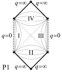 Figure 1
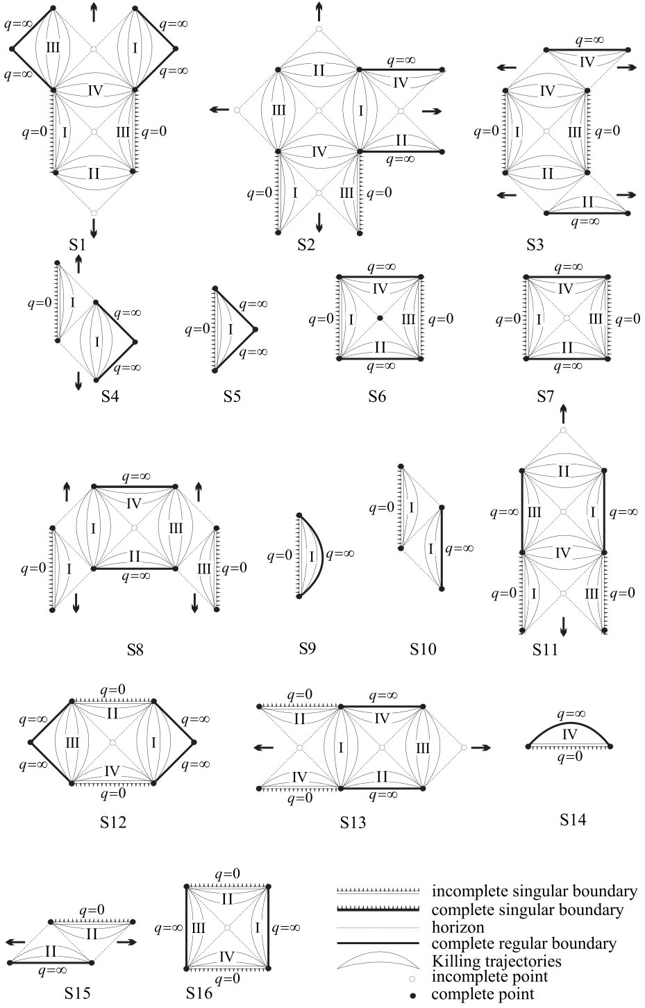 Figure 2
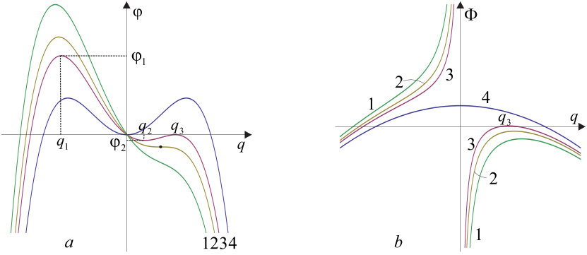 Figure 3
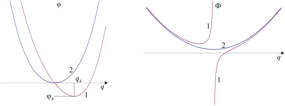 Figure 4
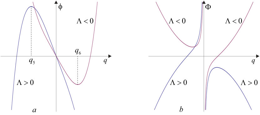 Figure 5
| S7 | ||||
| S11 | ||||
| S10 | ||||
| S9 | ||||
| S9 | ||||
| S14 | ||||
| S13 | ||||
| S15 | ||||
| S14 | ||||
| S16 |
Peer Reviews
No public reviews on file for this paper yet. If you reviewed it on a platform where reviews are public (OpenReview, ICLR, NeurIPS, ICML), you can paste yours below so the community can read it here.
Videos
No videos yet. Explain this paper in a talk, walkthrough, or lecture? Add one.
Global properties of warped solutions in General Relativity with
electromagnetic field and cosmological constant
D. E. Afanasev
High school N1561, ul. Paustovskogo, 6, kor. 2, 117464, Moscow
M. O. Katanaev
Steklov mathematical institute, ul. Gubkina, 8, Moscow, 119991, Russia E-mail: [email protected]: [email protected]
(20 March 2019)
Abstract
We consider general relativity with cosmological constant minimally coupled to electromagnetic field and assume that four-dimensional space-time manifold is the warped product of two surfaces with Lorentzian and Euclidean signature metrics. Einstein’s equations imply that at least one of the surfaces must be of constant curvature. It means that the symmetry of the metric arises as the consequence of equations of motion (‘‘spontaneous symmetry emergence’’). We give classification of global solutions in two cases: (i) both surfaces are of constant curvature and (ii) the Riemannian surface is of constant curvature. The latter case includes spherically symmetric solutions (sphere with -symmetry group), planar solutions (two-dimensional Euclidean space with -symmetry group), and hyperbolic solutions (two-sheeted hyperboloid with -symmetry). Totally, we get 37 topologically different solutions. There is a new one among them, which describes changing topology of space in time already at the classical level.
1 Introduction
There are many well known exact solutions in general relativity (see, i.e. [1]). To give physical interpretation of any solution to Einstein’s equation, we must know not only the metric satisfying equations of general relativity but the global structure of space-time. By this we mean a pair , where is the four-dimensional space-time manifold and is the metric on such, that manifold is maximally extended along geodesics: any geodesic line on either can be continued to infinite value of the canonical parameter in both directions, or it ends up at a singular point, where one of the geometric invariants becomes infinite. The famous example is the Kruskal–Szekeres extension [2, 3] of the Schwarzschild solutions. In this case, the space-time is globally the topological product of a sphere (spherical symmetry) with the two-dimensional Lorentzian surface depicted by the well known Carter–Penrose diagram. The knowledge of this global structure of space-time allows one to introduce the notion of black and white holes.
The famous Reissner–Nordström solution [4, 5], which is the spherically symmetric solution of Einstein’s equations with electromagnetic field, is also known globally. There are three types of Carter–Penrose diagrams: the Reissner-Nordström black hole, extremal black hole and naked singularity. The type of the Carter–Penrose diagram depends on the relation between mass and charge parameters. The spherically symmetric exact solution of Einstein’s equations with electromagnetic field and cosmological constant is known locally but not analyzed in full detail globally. In this paper, in particular, we give complete classification of global spherically symmetric solutions of Einstein’s equations with electromagnetic field and cosmological constant, which depends on relations between three parameters: mass, charge, and cosmological constant. We show that there are 16 different Carter–Penrose diagrams in the spherically symmetric case.
In fact, more general classification is given. We do not assume that solutions have any symmetry from the very beginning. Instead, we require the space-time to be the warped product of two surfaces: , where and are two two-dimensional surfaces with Lorentzian and Euclidean signature metrics, respectively. As the consequence of the equations of motion, at least one of the surfaces must be of constant curvature. In this paper, we consider the cases when (i) both surfaces and are of constant curvature and when (ii) only surface is of constant curvature. In the latter case, there are three possibilities: is the sphere (the spherical symmetry), the Euclidean plane (the Poincare symmetry), and the two-sheeted hyperboloid (the Lorentzian symmetry). We see that the symmetry of solutions is not assumed from the beginning but arise as the consequence of the equations of motions. This effect is called ‘‘spontaneous symmetry emergence’’. We classify all global solutions by drawing their Carter–Penrose diagrams for surface depending on relations between mass, charge, and cosmological constant. Totally, there are 4 different Carter–Penrose diagrams in case (i) and 33 globally different solutions in case (ii).
Moreover, we prove that there is the additional forth Killing vector field in each case. This is a generalization of Birkhoff’s theorem stating that any spherically symmetric solution of vacuum Einstein’s equations must be static. The existence of extra Killing vector field is proved for , , and symmetry groups.
This paper follows the classification of global warped product solutions of general relativity with cosmological constant (without electromagnetic field) given in [6]. The Carter–Penrose diagrams are constructed using the conformal block method described in [7].
As in [6], we assume that space-time is the warped product of two surfaces: , where and are surfaces with Lorentzian and Euclidean signature metrics, respectively. Local coordinates on are denoted by , , and coordinates on the surfaces by Greek letters from the beginning and middle of the alphabet:
[TABLE]
That is . Geometrical notions on four-dimensional space-time are marked by the hat to distinguish them from notions on surfaces and , which appear more often.
We do not assume any symmetry of solutions from the very beginning.
Four-dimensional metric of the warped product of two surfaces has block diagonal form by definition:
[TABLE]
where and are some metrics on surfaces and , respectively, and are scalar (dilaton) fields on and .
The Ricci tensor components for metric (1) are
[TABLE]
where, for brevity, we introduce notation
[TABLE]
Here and in what follows symbol denotes covariant derivative with the corresponding Christoffel’s symbols. The four-dimensional scalar curvature is
[TABLE]
where
[TABLE]
Scalar curvatures of surfaces and are denoted by and , respectively.
2 Solution for electromagnetic field
We assume that electromagnetic field is minimally coupled to gravity. Then the action takes the form
[TABLE]
where is the scalar curvature for metric , , is a cosmological constant, and is the square of electromagnetic field strength:
[TABLE]
Here, are components of electromagnetic field potential. For brevity, gravitational and electromagnetic coupling constants are set to unity.
Variation of action (6) with respect to metric yields four-dimensional Einstein’s equations:
[TABLE]
where
[TABLE]
is the electromagnetic field energy-momentum tensor. Variation of the action with respect to electromagnetic field yields Maxwell’s equations:
[TABLE]
where
[TABLE]
To simplify the problem, we assume that the four-dimensional electromagnetic potential consists of two parts:
[TABLE]
where and are two-dimensional electromagnetic potentials on surfaces and , respectively. Then the electromagnetic field strength becomes block diagonal:
[TABLE]
where
[TABLE]
are strength components for two-dimensional electromagnetic potentials.
In what follows, the raising of Greek indices from the beginning and middle of the Greek alphabet is performed by using the inverse metrics and . Therefore
[TABLE]
where and are dilaton fields entering four-dimensional metric (1). The square of four-dimensional electromagnetic field strength is
[TABLE]
In the case under consideration, Maxwell’s Eqs. (9) for lead to equality
[TABLE]
A general solution to these equations has the form
[TABLE]
where is the totally antisymmetric second rank tensor density. The factor 2 is introduced in the right hand side of general solution for simplification of subsequent formulae. This solution is rewritten as
[TABLE]
where is now the totally antisymmetric second rank tensor.
If , then Maxwell’s Eqs. (9) yield the equality
[TABLE]
Its general solution is
[TABLE]
Now the four-dimensional electromagnetic energy-momentum tensor (8) is easily calculated. It is block diagonal:
[TABLE]
where
[TABLE]
Note that we do not need the electromagnetic potentials and for the calculation of the energy-momentum tensor. It is sufficient to know strengthes (12) and (13).
Now we have to solve Einstein’s Eqs. (7) with right hand side (14). Since energy-momentum tensor depends only on the sum , we set to simplify formulae. In the final answer, this constant is easily reconstructed by substitution .
In what follows, we consider only the case , because the case was considered in [6] in full detail.
3 Einstein’s equations
The right hand side of Einstein’s Eqs. (7) is defined by general solution of Maxwell’s equations, which leads to electromagnetic energy-momentum tensor (14). The trace of Einstein’s equations can be easily solved with respect to the scalar curvature:
[TABLE]
which does not depend of the electromagnetic field, because the trace of the electromagnetic field energy-momentum tensor equals zero. After elimination of the scalar curvature, Einstein’s equations are simplified:
[TABLE]
For indices values , , and , these equations yield the following system of equations:
[TABLE]
where and are Ricci tensors for two-dimensional metrics and , respectively, and are two-dimensional covariant derivatives with Christoffel’s symbols on surfaces and , or , which is clear from the context. Sure, the equalities and hold. But we keep the symbol of covariant derivative for uniformity.
For subsequent analysis of Einstein’s equations, we extract the traces and traceless parts from Eqs. (16) and (17). Then the full system of Einstein’s equations takes the form
[TABLE]
where , , and are scalar curvatures of two-dimensional surfaces and for metrics and , respectively. In the above formulae, we used equalities and valid in two dimensions.
The last Eq. (23), which corresponds to mixed values of indices in Einstein’s equations results in strong restrictions on solutions. Namely, as in the case without electromagnetic field, there are only three cases:
[TABLE]
We shall see in what follows, that this leads to ‘‘spontaneous symmetry emergence’’.
Now we consider the first two cases in detail.
4 Product of constant curvature surfaces
The most symmetric solutions of Einstein’s equations with electromagnetic field in the form of the product of two constant curvature surfaces arise in case A (24), when both dilaton fields are constant. If and are constant, then Eqs. (19) and (20) are identically satisfied, and Eqs. (21) and (22) take the form
[TABLE]
where
[TABLE]
are Gaussian curvatures of surfaces and , respectively. It means that both surfaces are of constant curvature in case A. The metric on each surface is invariant under three-dimensional transformation group.
In stereographic coordinates on both surfaces, the metric of four-dimensional space-time takes the form
[TABLE]
where and .
We can put and by rescaling coordinates. One has also to redefine the constant of integration . We choose and for the metric signature to be . Then the Gaussian curvatures are
[TABLE]
There are four qualitatively different cases for topologically inequivalent global solutions depending on relations between cosmological constant and charge:
[TABLE]
where is the one sheet hyperboloid (more precisely, its universal covering) embedded in three-dimensional Minkowskian space , is the Lobachevsky plane (the upper sheet of two-sheeted hyperboloid embedded in ), and is the two-dimensional sphere. From topological point of view the third and fifth cases in Eq. (28) coincide. Therefor there are only four topologically inequivalent global solutions of Einstein’s equations in the form of direct product of two constant curvature surfaces. Note that for , there are only three topologically inequivalent solutions [6].
All solutions have exactly six Killing vector fields and belong to type in Petrov’s classification.
The cases of other signatures of four-dimensional metric for and are analysed similarly. Qualitative properties of global solutions are the same.
We see that symmetry properties in this case are not imposed from the very beginning but arise as the result of solution of equations of motion. This effect is called ‘‘spontaneous symmetry emergence’’.
5 Solutions with spatial symmetry
The dilaton field is constant in second case B (24). Without loss of generality, we put . Then Einstein’s equations (19)–(23) take the form
[TABLE]
Consider Eq. (30). The scalar curvature depends on coordinates on surface , whereas all other terms depend on coordinates on surface . For this equation to be fulfilled, it is necessary that equation holds. It means that surface must be of constant curvature as the consequence of Einstein equations. Therefor the four-dimensional metric of space-time has at least three independent Killing vector fields. So, there is spontaneous symmetry emergence.
Let us put . Then Eq. (30) is
[TABLE]
Excluding the case A considered in the previous section, we proceed further assuming on the whole .
Proposition 5.1**.**
Equation (32) is the first integral of Eqs. (29) and (31).
Proof.
Differentiate Eq. (32) and use the equality
[TABLE]
valid for any covector field , to change the order of derivatives in the first term:
[TABLE]
Now exclude derivatives and using Eqs. (29) and (30) in the first and fourth terms on the right hand side. After rearranging terms, the sum of the first and fourth terms takes the form
[TABLE]
Taking all terms together, we obtain
[TABLE]
Since , it implies the statement of the proposition. ∎
The proof of the proposition implies that it is sufficient to solve Eqs. (29) and (32), Eq. (31) being satisfied automatically.
To solve Eqs. (29) and (32) explicitly, we fix the conformal gauge for metric on Lorentzian surface :
[TABLE]
where is the conformal factor depending on light cone coordinates , on . The respective four dimensional metric is
[TABLE]
where is the metric on the Riemannian surface of constant curvature , , or . The sign of the conformal factor is not fixed for the present.
For and the signature of metric (35) is . If we change the sign of , the signature of the metric becomes . The same transformation of the signature can be achieved by changing the overall sign of the metric , and interchanging the first two coordinates, . Einstein’s equations with cosmological constant and electromagnetic field (15) are not invariant with respect to these transformations with simultaneous changing the sign of the cosmological constant, because the right hand side changes its sign. Therefor, for , we have to consider two cases:
[TABLE]
This is the difference for Einstein’s equations without electromagnetic field considered in [6].
5.0.1 Metric signature
For and , we introduce convenient parameterization
[TABLE]
Afterwards, we obtain the full system of equations:
[TABLE]
The first two equations which do not depend on the electromagnetic field imply the following assertion.
Proposition 5.2**.**
If , then the function depends only on timelike coordinate . If , then the function depends only on spacelike coordinate . And the following equality holds
[TABLE]
where prime denotes differentiation on the argument (either , or ).
This proposition provides a general solution to equations (37) and (38) up to conformal transformations. This statement is proved in [6, 8].
Thus, we can always choose coordinates in such a way that and depend simultaneously on timelike or spacelike coordinate
[TABLE]
It means that two-dimensional metric (34) and consequently four-dimensional metric (35) have the Killing vector or , as the consequence of equations (37) and (38). We call these solutions homogeneous and static, respectively, though it is related to the fixed coordinate system. The existence of additional Killing vector is the generalization of Birkhoff’s theorem [9] stating that arbitrary spherically symmetric solution of vacuum Einstein’s equations must be static. (This statement was previously published in [10].) The generalization includes the addition of electromagnetic field, and, in addition, the existence of extra Killing vector is proved not only for spherically symmetric solution , but also for solutions invariant with respect to and transformation groups.
We are left to solve equation (39). In static, , and homogeneous, , cases, equation (39) takes the form
[TABLE]
To integrate the derived equations, one has to express through using equation (40) and removing the modulus sign.
We consider the static case , and in detail. Then Eq. (42) together with Eq. (40) reduces to
[TABLE]
It can be easily integrated:
[TABLE]
where is an integration constant, which coincides with mass in the Schwarzschild solution. Differentiating the left hand side and dividing it by , we obtain equation
[TABLE]
Since in the case under consideration, it implies expression for the conformal factor through variable :
[TABLE]
If , and , then the similar integration yields
[TABLE]
where the same conformal factor (44) stands in the right hand side. This case can be united with the previous one by re-writing equation for in the form
[TABLE]
The modulus sign in the left hand side means that if is a solution, then the function is also the solution.
The static case for is integrated in the same way:
[TABLE]
If solution is homogeneous, and , , then integration of Eq. (43) yields the equality
[TABLE]
That is the conformal factor must be identified with the right hand side
[TABLE]
We denote the expression for the conformal factor through by hat because in homogeneous case it differs by the sign. Thus, homogeneous solutions of Einstein’s equations can be written in the form
[TABLE]
If the conformal factor is negative, then the signature of the metric is . In this case, we return to the previous signature after substitution . This transformation allows us to unite static and homogeneous solutions by taking the modulus of the conformal factor in the expression for metric (35). Then a general solution of vacuum Einstein’s equations with electromagnetic field (7) in the corresponding coordinate system takes the form
[TABLE]
where the conformal factor is given by Eq. (44). Here the variable depends on (static local solution) or (homogeneous local solution) through the differential equation
[TABLE]
where the sign rule holds:
[TABLE]
Thus the four-dimensional Einstein’s equations imply that there is the metric with one Killing vector field on surface which was considered in full detail in [7]. Now we can construct global solutions (maximally extended along geodesics) of vacuum Einstein’s equations using the conformal block method. The number of singularities and zeroes of conformal factor (44) depends on relations between constants , , , and . Therefor there are many qualitatively different global solutions, which are considered in next sections.
Conformal factor (44) has one singularity: the second order pole at . Therefor according to the rules formulated in [7, 8] every global solution correspond to one of the intervals or . The form of conformal factor (44) implies that these global solutions are obtained one from the other by the transformation . Hence, without loss of generality, we describe global solutions corresponding to both intervals but positive values of .
Because conformal factor is a smooth function for , all arising Lorentzian surfaces and metrics on them are smooth.
To conclude the section we compute geometrical invariants which show that obtained solution of Einstein’s equations are nontrivial. First, we compute the scalar curvature of the surface . Equations (30) and (31) imply
[TABLE]
Since
[TABLE]
both for static and homogeneous solutions, the final expression is
[TABLE]
It does not depend on Gaussian curvature of Riemannian surface and is singular for if and/or .
5.0.2 Metric signature
If , then the signature of the metric is opposite , and we introduce parameterization
[TABLE]
instead of Eq. (36). Performing the same calculation as in the previous section, we obtain the first order equation for :
[TABLE]
where is an integration constant and
[TABLE]
Here we must take into account that for getting the signature we have to make interchanging . We see that for drawing the Carter–Penrose diagram one has to simply make replacement and as compared to signature .
Now we describe all spatially symmetric global solution of Einstein’s equations with electromagnetic field which are defined by zeroes and their types of the conformal factor .
5.1 Spherically symmetric solutions
In the considered case, global spherically symmetric solutions, that is pairs , have the form , where is the maximally extended Lorentzian surface which is depicted by the Carter–Penrose diagram. Four-dimensional metric on has the form (50), where is the metric on sphere for signature . If the signature is opposite , then we have to replace and in the conformal factor and change the sign of in metric (50). Due to the existence of one Killing vector on Lorentzian surface , we are able to classify all global solutions. To construct Carter–Penrose diagrams, we use the conformal block method described in [7] (see also, [8]). First, we consider solutions of signature , and then with signature .
5.1.1 Metric signature
If the metric signature is , then the conformal factor is
[TABLE]
where we introduced the auxiliary function
[TABLE]
which is needed for further analysis. The case was analyzed in [6]. Therefor, we classify solutions for . Without loss of generality, we consider the case , because only enters the conformal factor.
Conformal factor (56) has the second order pole at zero and the following asymptotic at infinity
[TABLE]
If cosmological constant is equal to zero, then metric is asymptotically flat. For and , we have asymptotically de Sitter and anti-de Sitter spacetime, respectively.
A global solution corresponds to one of the intervals or and , because the curvature has singularity (53) at zero, and space-time is not extendable through this point. Roots of conformal factor (56) correspond to horizons of space-time, and Carter–Penrose diagrams are defined by the number and type of zeroes of the conformal factor [7]. Thus we have to analyse the number and type of zeroes of conformal factor (56) for all possible values of constants , , and .
Note that conformal factor (56) is invariant with respect to transformation
[TABLE]
Therefor, instead of constructing global solutions on the interval for all values of , we restrict ourselves only for nonnegative , but on two intervals and . This simplifies the analysis of the conformal factor.
We start with the simplest and well known case .
5.1.2 Metric signature . The case .
If cosmological constant vanishes, then zeroes of conformal factor (56) are defined by the quadratic equation
[TABLE]
which has two roots:
[TABLE]
The Reissner–Nordström solution. For , there are two positive simple roots. This solution is called the Reissner–Nordström solution [4, 5] and depicted by the Carter–Penrose diagram S1 shown in Fig.1. It was also found by H. Weyl [11]. The solution has two horizons at and and naked timelike singularity at . The conformal factor tends to unity at infinity, and, consequently, the Reissner–Nordström solution is asymptotically flat. Arrows on the diagram show directions in which the solution can be periodically extended in time. Instead of periodic extension, there is the possibility to identify the opposite horizons. The singularity at is timelike, and an observer can approach it as close as he likes in conformal blocks I or III, and then enter universe III or I by going through conformal block IV. Therefor, the Reissner–Nordström solution does not describe a black hole.
Extremal black hole. For , the conformal factor is
[TABLE]
It has one positive root of second order at . The corresponding Carter–Penrose diagram is shown in Fig.1, S4. It is called extremal black hole, though there is no any black hole since the singularity is timelike and horizon surrounding the singularity is absent. There is also space-reflected diagram.
Naked singularity. For , horizons are absent, and we have naked singularity shown in Fig.1, S5. There is also space-reflected diagram.
5.1.3 Metric signature . The case .
For positive cosmological constant, zeroes of the conformal factor are defined by the fourth order equation
[TABLE]
where function is given by the fourth order polynomial (57). To draw Carter–Penrose diagrams, we do not need to know exact position of zeroes. We have to know only their existence and type. Therefor, we analyze function qualitatively and then move its graphic up, which corresponds to increasing value of .
First, we differentiate function (60):
[TABLE]
The asymptotics of function () and its derivatives for and are easily found:
[TABLE]
Zeroes of function require more work. As we see later, their number does not exceed three. To find the types of zeroes, we have to know local extrema of function , which become zeroes of order two or three after shifting on .
Local extrema of function are defined by cubic equation (the solution is given, i.e. in [12])
[TABLE]
There are three qualitatively distinct cases depending on the value of constant
[TABLE]
Namely,
[TABLE]
We start with the simplest case . This equality implies restriction on ‘‘mass’’:
[TABLE]
Moreover, roots of Eq. (63) take the simple form:
[TABLE]
As we see, there are one simple negative root and one positive root of second order for positive ‘‘mass’’ (65).
If inequality holds, then real roots of cubic equation (63) are (see, i.e., [12])
[TABLE]
where
[TABLE]
Since we consider only nonnegative , then \alpha\in\big{[}\frac{\pi}{2},\frac{3\pi}{2}\big{]}. It implies existence of one negative root and two positive: and . We enumerate the zeroes in Eq. (67) in such a way, that, in the limit
[TABLE]
they take values (66).
If , then we have only one negative root . Its exact position can be written but it is not needed.
Figure 2, a, shows qualitative behavior of function for and different values of .
Now, to construct all global solutions which exist in the theory for signature , we have to analyse zeroes of conformal factor , qualitative behavior of which for is shown in Fig.2, b. Zeroes of the conformal factor and their type coincide with that of function . Therefor, we have to shift up curves 1–4 in Fig.2, a, on to analyse its qualitative behavior. The number and type of zeroes depend on curves 1–4 and on the value of the shift . All possible Carter–Penrose diagrams are drawn in Fig.1.
The conformal factor depicted by curve 4 in Fig.2, b, does not have zero at . It corresponds to de Sitter space, and is degenerate at this presentation of the problem (, ), which is not considered here because of the assumption .
For qualitative description of behavior of the conformal factor, we introduce notation:
[TABLE]
where is the maximum, is local minimum, and is local maximum of the auxiliary function . One can easily verify, that, for and , the maximum is positive: . On positive half line , the local minimum is always negative: , and local maximum can take negative as well as positive values:
[TABLE]
When Eq. (65) holds, local minimum and maximum coincide: . Now we list all possibilities in the considered case.
Three horizons. Under condition
[TABLE]
the conformal factor has three simple zeroes on positive half line. The corresponding Carter–Penrose diagram of surface is given by S2 in Fig.1. Here we have two timelike naked singularities. Arrows show that this diagram can be either periodically continued in space- and timelike directions, or opposite horizons can be identified. If we identify horizons in one direction, them topologically the surface is a cylinder. If identification is performed in both directions, then it is a torus.
One simple horizon and timelike singularity. The conformal factor has one simple zero on positive half line under the following conditions:
[TABLE]
This global solution is depicted by the Carter–Penrose diagram S7. It has timelike singularity.
Triple horizon. Under conditions:
[TABLE]
local maximum and minimum of auxiliary function coincide: , and the conformal factor has zero of third order at point (triple horizon). This case is depicted by diagram S6. It coincides with diagram S7, but there is one important difference: the saddle point in the center of the diagram is geodesically complete.
This diagram is interesting from physical standpoint. Consider a spacelike section of this diagram. If the section does not go through the saddle point, which is located in the center of the diagram, then it is an interval of finite length with singular ends where two-dimensional curvature becomes infinite. If the space section goes through the saddle point then it is the union of two half-infinite intervals, because the central point in the center of the diagram is the space infinity. If we introduce now global evolution parameter , for instance, vertical line on the diagram, then topology of space sections change during evolution: for some value of , there are two half-infinite intervals instead of one finite interval. This example shows that changing topology of space in time can occur already at the classical level. This type of diagram appeared first in two-dimensional gravity with torsion [13].
Two horizons with double local minima. Under conditions:
[TABLE]
the conformal factor has one zero of second order at point and one simple simple zero at some point lying to the right from . This solution is depicted by Carter–Penrose diagram S8 with two timelike singularities, which can be periodically extended in timelike direction.
Two horizons with double local maximum. Under conditions:
[TABLE]
the conformal factor has one double zero at and one simple zero at some point lying to the left from . This solution corresponds to Carter–Penrose diagram S3 with two timelike singularities, which can be periodically extended in spacelike direction.
5.1.4 Metric signature . The case .
For negative cosmological constant, the conformal factor have the same form and asymptotics remain the same (62). Equation (63) and constant (64), defining the roots, do not change. We see that values of constant are positive for all and . Consequently, Eq. (63) has only one nonnegative real root. Moreover, now branches of auxiliary function are directed upwards as shown in Fig.3, and three new Carter–Penrose diagrams appear in the spherically symmetric case.
The conformal factor depicted by curve 2 in Fig.3, b, has zero at point . It corresponds to anti-de Sitter space and is the degenerate case in the problem under consideration (, ).
Now we list all possibilities for negative cosmological constant.
Timelike singularity. Under conditions:
[TABLE]
the conformal factor does not have zeroes, and, consequently, horizons are absent. In this case, the Carter–Penrose diagram has the lens form S9 in Fig.1. There is also space-reflected diagram.
Naked singularity. Under conditions:
[TABLE]
the conformal factor has one positive root of second order at the minimum of the auxiliary function at . In this case, the Carter–Penrose diagram is S10 in Fig.1. In contrast to the naked singularity S4, the right complete infinity is timelike. It is due to asymptotic of the conformal factor at infinity, because space-time is asymptotically anti-de Sitter for . There is also space-reflected diagram.
Timelike singularity and two horizons. Under conditions:
[TABLE]
the conformal factor has two zeroes. In this case, the Carter–Penrose diagram is given by S11 in Fig.1. This solution can either be periodically extended in timelike direction or opposite horizons can be identified. In contrast to diagram S1, space infinities are timelike, which is due to asymptotic at infinity.
Thus we classified all spherically symmetric global solutions of Einstein’s equations with electromagnetic field for metric signature . We see, that all solutions of signature contain timelike singularity. Totally, we get 11 topologically inequivalent solutions S1–S11. It is possible to give more subtle classification taking into account existence of degenerate and oscillating geodesics. The latter appears, if the conformal factor has local extremum inside one of the conformal blocks. This classification was given for global solutions of two-dimensional gravity with torsion [13].
5.1.5 Metric signature
If the signature is opposite, the conformal factor has the form (56) but with the replacement . It means that auxiliary function in Figs. 2 and 3, a, remains the same, but we have to move it downwards instead of upwards. There are 5 new Carter–Penrose diagrams.
We start with the simplest case.
5.1.6 Metric signature . The case .
In the considered case, zeroes of the conformal factor are defined by quadratic equation
[TABLE]
which has two roots:
[TABLE]
It implies inequalities and for . Therefor, there is one simple horizon for any . Consequently, the Carter–Penrose diagram has exactly the same form as for Schwarzschild black hole S12 in Fig.1.
5.1.7 Metric signature . The case .
Auxiliary function is the same (57), but it has to be moved on downwards. For positive cosmological constant, the qualitative behavior of the auxiliary function is shown in Fig.2, a.
Spacelike singularity. Under conditions:
[TABLE]
the conformal factor does not have roots. In this case, there is spacelike singularity without horizons. Its Carter–Penrose diagram is S14 in Fig. 1. There is also time-reflected diagram.
Spacelike singularity with two horizons. Under conditions:
[TABLE]
the conformal factor has two simple zeroes, and, consequently, two horizons. Moreover the singularity at is spacelike. This solution is depicted by diagram S13 in Fig. 1. It can be either periodically extended in spacelike direction, or we can identify the opposite horizons. This solution describes white and black holes, which are periodically located in spacelike directions. Moreover, if an observer is located in the domain IV, he has the opportunity either to live forever, or to fall on one of two black holes.
Spacelike singularity with one double horizon. Under conditions:
[TABLE]
the conformal factor has one double zero, and the singularity is spacelike. This global solution is given by the Carter–Penrose diagram S15 in Fig. 1, which can be periodically extended in spacelike direction. This solution describes the collection of black and white (after time reflection) holes. As in the previous case, an observer in domain II has the choice either to live forever or to fall on one of two black holes. There is also time-reflected diagram.
5.1.8 Metric signature . The case .
For negative cosmological constant and signature , the auxiliary function has previous form and is shown in Fig.3. To find zeroes, its graphic must be moved downwards. Thus for all values of parameters:
[TABLE]
it has one simple zero. This global solution is given by diagram S16 in Fig. 1. In this case we have asymptotically anti-de Sitter black hole. Note, that, for positive mass, the space-time has degenerate and oscillating geodesics, because local minimum exists for . For these geodesics are absent.
Thus, for metric signature , there are only 5 topologically different global solutions S12–S16. All singularities in this case are spacelike and correspond either to black or white holes.
5.2 Planar solutions
If Gaussian curvature of surface equals to zero, then it is either the Euclidean plane , or a cylinder, or a torus (after factorization). Thus, there is spontaneous symmetry arising if the surface is Euclidean plane . That is, the space-time metric becomes invariant with respect to transformation group on the equations of motion. In Schwarzschild coordinates , it is written in the form (for , corresponding to signature ):
[TABLE]
where
[TABLE]
To draw Carter–Penrose diagrams for Lorentzian surface , we have to analyse zeroes and asymptotics of conformal factor . For , we have the second order pole at zero and asymptotic at infinity
[TABLE]
On intervals and , the conformal factor is smooth, and, consequently, every global solution corresponding to one of these intervals is smooth. As for spherically symmetric solutions, we consider positive on both intervals due to the symmetry transformation .
We start with the simplest case.
5.2.1 Metric signature . The case .
The conformal factor is
[TABLE]
It has obviously one simple zero
[TABLE]
Moreover, there are only two cases.
Timelike singularity and one horizon. Under conditions:
[TABLE]
the conformal factor has one simple positive zero. The corresponding Carter–Penrose diagram is P1 in Fig. 4. This diagram has the same form as the Schwarzschild black hole S12 but turned over on .
Naked singularity. Under conditions:
[TABLE]
positive roots of the conformal factor are absent, and we have naked singularity S5 in Fig. 1. ∎
To find zeroes for nonzero cosmological constant , we introduce auxiliary function representing the conformal factor for signature in the form
[TABLE]
where
[TABLE]
For the opposite signature, , it is needed to make replacement . We see that on intervals and the number and type of zeroes of the conformal factor coincide with zeroes of numerator . It means that auxiliary function must be shifted either downwards (signature ), or upwards (signature ).
Auxiliary function (87) has two real roots:
[TABLE]
and two complex conjugate roots which do not interest us. Qualitative behavior of the auxiliary function and corresponding conformal factor are shown in Fig. 5. Position of extrema of the auxiliary function is defined by the equality
[TABLE]
We denote them by and for and , respectively (see. Fig. 5, a).
The maximal and minimal values of the auxiliary function are denoted by
[TABLE]
It is clear, that for and for .
Detailed analysis show that Carter–Penrose diagrams for all planar solutions for were already met in the spherically symmetric case. Therefor, to save space, we give classification of all planar solutions in table 1.
Note, that diagrams S7, S9, S10 and S11 differ from diagrams S16, S14, S15 and S13 by the turn on degrees, respectively.
6 Hyperbolic global solutions
If Gaussian curvature of surface is negative, , then the surface is two-sheeted hyperboloid , more precisely, the upper sheet of two-sheeted hyperboloid (the Lobachevsky plane). It is the universal covering surface for closed Riemannian surfaces of genus two and higher. If , then the isometry group is the Lorentz group . In this case, the metric in Schwarzschild coordinates for signature has the form
[TABLE]
where
[TABLE]
The conformal factor for this metric differs from that in the spherically symmetric case (56) by the transformation
[TABLE]
In addition, transformation corresponds to signature change of the metric, . Since we have already described global spherically symmetric solutions for all values of and , all hyperbolic solutions are obtained from spherically symmetric ones by simple rotation of Carter–Penrose diagrams by , which corresponds to transformation . In this way we get 16 additional Carter–Penrose diagrams.
7 Conclusion
We assumed that four-dimensional space-time is the warped product of two surfaces, , and find a general solution of Einstein’s equations with cosmological constant and electromagnetic field. These solutions are well known locally and partly globally. We give classification of all global solutions in the case when surface is of constant curvature. Totally, there are 37 topologically different global solutions. These solutions in case B have four Killing vector fields, three of them corresponding to symmetry of the metric on constant curvature surface . They are generators of isometry groups , , and in cases when surface is a sphere , Euclidean plane , and two-sheeted hyperboloid , respectively. The fourth Killing vector generalizes Birkhoff’s theorem. In all cases, there is ‘‘spontaneous symmetry emergence’’ because the existence of Killing vector fields was not assumed at the beginning, and their appearance is the consequence of Einstein’s equations. Most probably, part of the constructed solutions are not satisfactory from physical point of view. For example, for given signs in the Lagrangian and signature of the metric , the Carter–Penrose diagram for charged black hole coincide with the Schwarzschild solution. However, the quadratic form of momenta in the canonical Hamiltonian for physical degrees of freedom is not positive definite (ghosts appearance), and this solution have to be discarded as unphysical. Nevertheless, the given classification of global solutions of Einstein’s equations in the form of warped product of two surfaces is important, because we must know what is to be discarded.
The reference list from the paper itself. Each links out to its DOI / PubMed record.
- 1[1] D. Kramer, H. Stephani, M. Mac Callum, and E. Herlt. Exact Solutions of the Einsteins Field Equations . Deutscher Verlag der Wissenschaften, Berlin, 1980.
- 2[2] M. D. Kruskal. Maximal extension of Schwarzschild metric. Phys. Rev. , 119(5):1743–1745, 1960.
- 3[3] G. Szekeres. On the singularities of a riemannian manifold. Publ. Mat. Debrecen , 7(1–4):285–301, 1960.
- 4[4] H. Reissner. Über die Eigengravitation des elektrischen Feldes nach der Einsteinschen Theorie. Ann. Physik (Leipzig) , 50:106–120, 1916.
- 5[5] G Nordström. On the energy of the gravitational field in einstein’s theory. Proc. Kon. Ned. Akad. Wet. , 20:1238–1245, 1918.
- 6[6] M. O. Katanaev, T. Klösch, and W. Kummer. Global properties of warped solutions in general relativity. Ann. Phys. , 276:191–222, 1999.
- 7[7] M. O. Katanaev. Global solutions in gravity. Lorentzian signature. Proc. Steklov Inst. Math. , 228:158–183, 2000.
- 8[8] M. O. Katanaev. Geometric methods in mathematical physics. Ver. 3, 2016. ar Xiv:1311.0733 [math-ph][in Russian].