Tipping point analysis of electrical resistance data with early warning signals of failure for predictive maintenance
Valerie Livina, Adam Lewis, Martin Wickham

TL;DR
This paper introduces a novel tipping point analysis method for electrical resistance data, providing early failure warnings in electronic components, which enhances predictive maintenance capabilities in automotive and aviation industries.
Contribution
The study applies a statistical physics framework to resistance time series, enabling earlier failure detection than traditional threshold-based methods.
Findings
Early warning signals detected significantly before conventional methods
Scaling properties of resistance data reveal critical transition points
Applicable to various electromagnetic measurements in power systems
Abstract
We apply tipping point analysis to measurements of electronic components commonly used in applications in the automotive or aviation industries and demonstrate early warning signals based on scaling properties of resistance time series. The analysis utilises the statistical physics framework with stochastic modelling by representing the measured time series as a composition of deterministic and stochastic components estimated from measurements. The early warning signals are observed much earlier than those estimated from conventional techniques, such as threshold-based failure detection, or bulk estimates used in Weibull failure analysis. The introduced techniques may be useful for predictive maintenance of power electronics, with industrial applications. We suggest that this approach can be applied to various electromagnetic measurements in power systems and energy applications.
Click any figure to enlarge with its caption.
 Figure 1
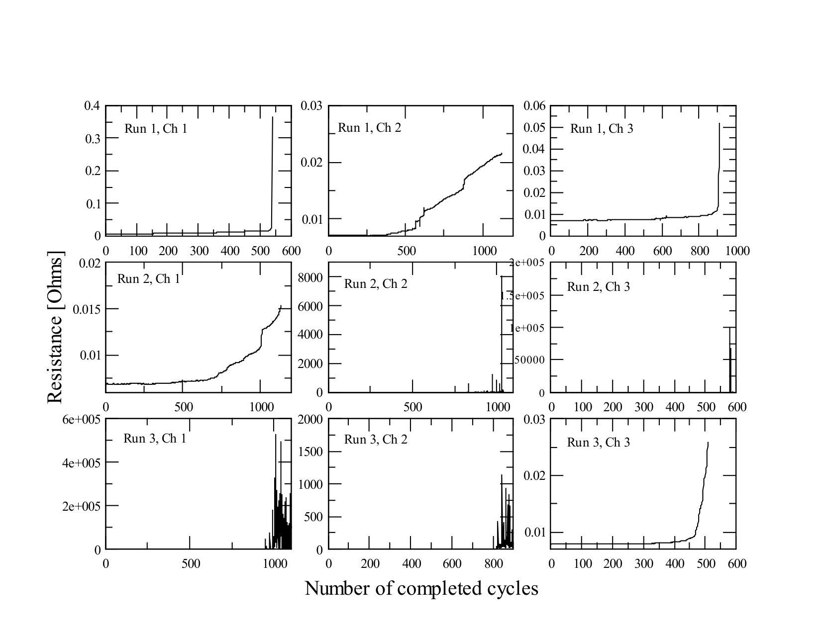 Figure 2
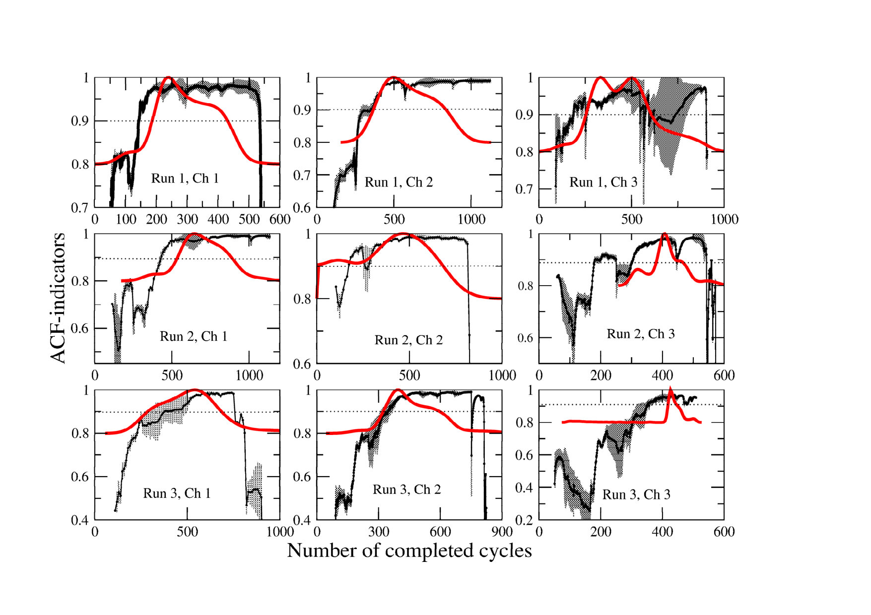 Figure 3
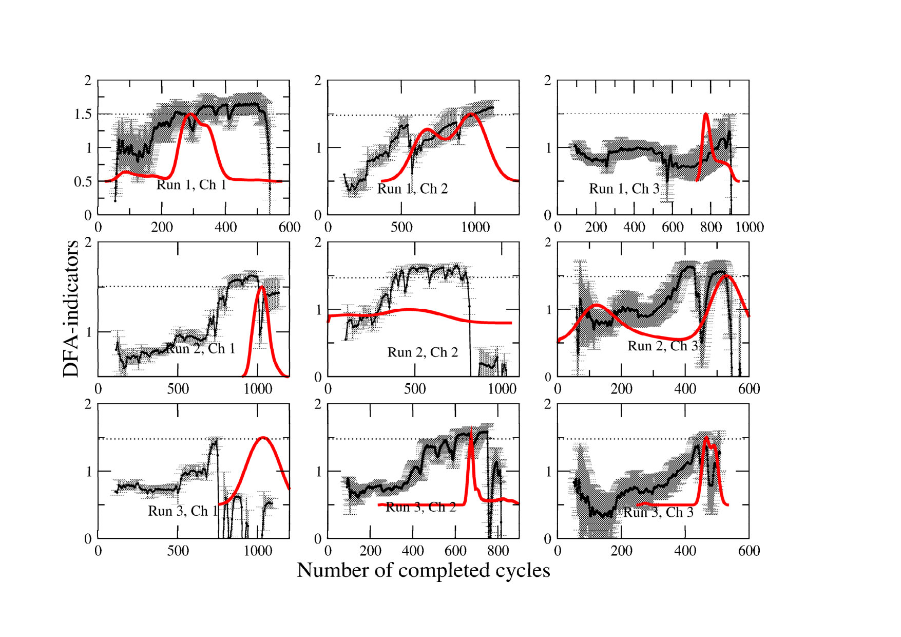 Figure 4
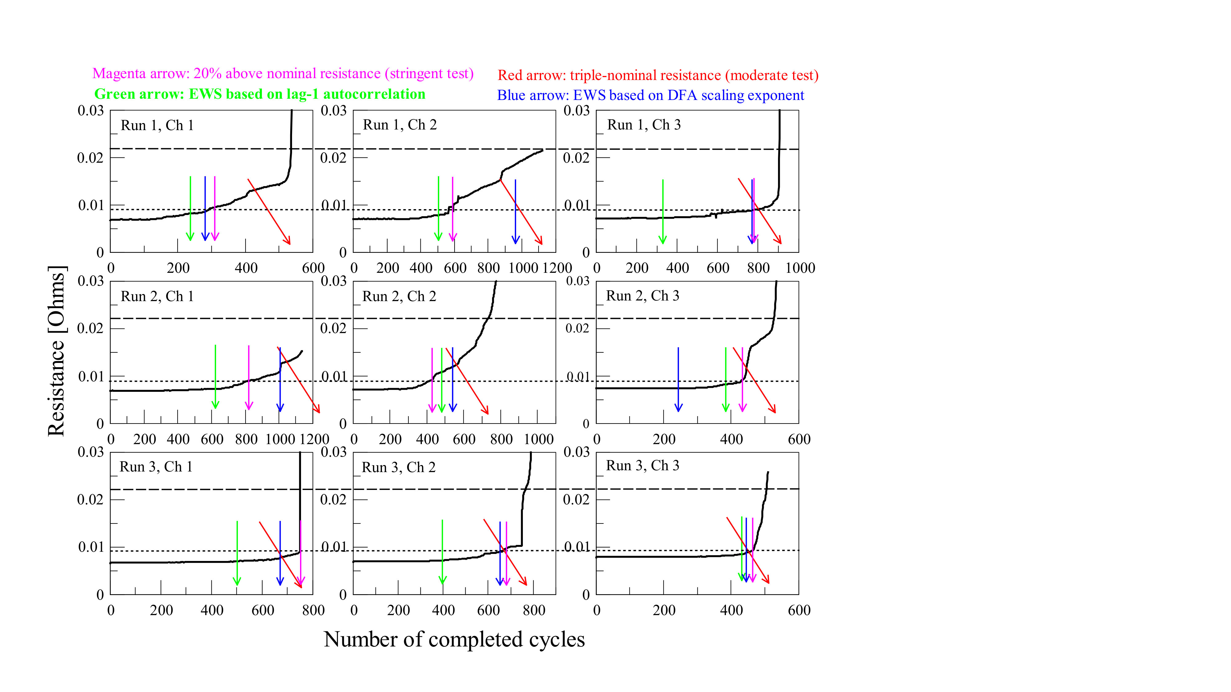 Figure 5
Peer Reviews
No public reviews on file for this paper yet. If you reviewed it on a platform where reviews are public (OpenReview, ICLR, NeurIPS, ICML), you can paste yours below so the community can read it here.
Videos
No videos yet. Explain this paper in a talk, walkthrough, or lecture? Add one.
Tipping point analysis of electrical resistance data
with early warning signals of failure for predictive maintenance
V. N. Livina1111Corresponding author, email:[email protected], A. P. Lewis1 and M. Wickham1
1National Physical Laboratory, Teddington, United Kingdom
Abstract
We apply tipping point analysis to measurements of electronic components commonly used in applications in the automotive or aviation industries and demonstrate early warning signals based on scaling properties of resistance time series. The analysis is based on a statistical physics framework with a stochastic model representing the system time series as a composition of deterministic and stochastic components estimated from measurements. The early warning signals are observed much earlier than those estimated from conventional techniques, such as threshold-based failure detection, or bulk estimates used in Weibull failure analysis. The introduced techniques may be useful for real-time predictive maintenance of power electronics, with industrial applications. We suggest that this approach can be applied to various electric measurements in power systems and energy applications.
1 Introduction
A significant challenge in the design and development of high-reliability electronic assemblies is in relating the results from testing to real-world performance. The key issue is that, due to the wide range of applications, standardised tests may not predict the range of harsh environments to which an electronic assembly will be exposed. As a consequence for high-reliability use, particularly in safety-critical applications, a common approach is to use a standardised test which utilises over stress conditions to accelerate failures.
Weibull reliability analysis [Scholz 1999] uses a parametric Weibull model to estimate a probability density and failure rate function based on the parameters of the distribution of parts failure, which provide information about the average behaviour of parts of expected quality. Factors such as time-to-first failure and analysis of Weibull distributions are used to give indications of when components/assemblies should be replaced.
However, since there are significant uncertainties in real stress conditions and quality of materials and manufacturing process, these indicators are based on the assumptions that are highly conservative: the Weibull plot gives the time to first failure (these are not conservative), however it is further used for stringent assumptions.
Therefore alternative methods are sought to give a more reliable indication of the remaining useful life. One method which has shown promise is the use of prognostic devices for monitoring solder joints [Chauhan et al 2014]. These can be components (e.g., zero-ohm resistors) which are incorporated into an electronic assembly and are designed to fail before any other component. As they are a part of the assembly, they will experience the same manufacturing, environmental and detrimental factors. As part of a feasibility study on a range methods for measuring the progression of failure for a solder joint (between a printed circuit board — PCB — and a zero-ohm resistor), an experiment was conducted which looked at the evolution of the DC resistance as the solder joint underwent thermal cycling.
The thermal cycling ageing process can cause cracks to form in the solder interconnect due to mismatches in the coefficients of thermal expansion between the substrate, contact pads, solder and components. These cracks cause discontinuities in the electrical circuit, although the resistance change during the crack initialisation tends to be minor until a failure event where the resistance increases significantly by several orders of magnitude, potentially to open circuit.
The hypothesis we test is whether small changes in electrical resistance and in the pattern of their fluctuations (such as short- and long-term memory) can be used as early warning indicators to predict impending failure events. Early warning signals (EWS) based on these changes proved to be of general applicability in generic dynamical systems, and bringing them into the area of predictive maintenance may serve as a cross-disciplinary advantage for the manufacturing industry. Conventionally, early warning signals are statistical indicators showing the approach of critical transitions in a dynamical system, which is often hidden by system fluctuations. The logic behind applying these indicators for failure diagnostics is that EWS indicators should be sensitive to changes in memory (i.e., long-term dependencies quantified by auto-correlations) in the measurements of devices, and this should happen earlier than any threshold-based transition is detected.
There are a number of industrial guides that suggest various thresholds and levels of tests (from stringent to moderate) of electronic components with different properties. Some of them operate values of up to 10,000 ohms and are specific to particular devices. Triple-nominal resistance is an empirical threshold that allows us to identify an abnormal increase of resistance before the hard open-circuit failure (which can be see as the vertical line in Figure 2). It is general enough to assess components with various characteristics. The hard failure with open circuit occurs later than the triple-nominal threshold, and our techniques detect the drift of the resistance variable even earlier.
This demonstrates that the proposed techniques are applicable to various systems, and can further be tuned for earlier detection if more stringent tests are necessary. The particular value of the methodology is that it analyses individual measurments of specific components and forewarns about individual failures rather than operates statistical averages.
Tipping points are critical transitions and bifurcations in time series data that may lead to another existing state of the dynamical system (such as change from regular dynamics to a failure), or to appearance and disappearance of system states, which may be crucial to condition monitoring. Time series analysis techniques that allow one to detect such tipping points may provide tools for predictive maintenance of dynamical systems, which is of particular importance in electronic devices that are related to control and safety.
Tipping points in dynamical systems have recently become a topic of high interest in the area of climate change; see, for example, [Lenton et al 2008]. Applications of the tipping point analysis have been found so far in geophysics [Livina and Lenton 2007, Livina et al 2010, Livina et al 2011, Livina et al 2012] [Prettyman et al 2018, Prettyman et al 2019], structure health monitoring [Livina et al 2014], as well as in ecology (see [Dakos et al 2012, Scheffer et al 2009] and references therein). There is a debate about various types of tipping [Ashwin et al 2012] and false alarms [Ditlevsen and Johnsen 2010], but for practical applications in industry, non-bifurcational transitions (without structural change of the dynamical system), may be as important as bifurcations and require adequate analytical tools and techniques of analysis. One of the advantages of the tipping point methodology is that it does not require extensive training datasets (unlike many other techniques of machine learning), and therefore can be useful in situations where there is limited operational data available, or where stress conditions are unknown.
A dynamical system with observed time series of measurements can be modelled by the following stochastic equation with state variable and time :
[TABLE]
where and are deterministic and stochastic components, respectively. The probability density of the system can then be approximated by a polynomial of even order (the so-called potential system, see [Livina et al 2010]). The stochastic component, in the simplest case, may be Gaussian white noise, although in real systems it is often more complex, for example, with power-law correlations, multifractal and other nonlinear properties.
Tipping points can be described in terms of the underlying system potential , whose state derivative, if it exists, defines the deterministic term in Equation (1), i.e. [Livina et al 2011]. If the potential structure (number of potential wells) changes, the tipping point is a genuine bifurcation. If the potential structure remains the same, while the trajectory of the system samples various states, such a tipping point is transitional. An example of such transition may be the record of global temperature, which has the same structure of fluctuations with a drift (under forcing or noise-induced). In practical terms, both transition and bifurcation may lead to catastrophic damage of devices, however, genuine bifurcations tend to have more gradual dynamics compared with abrupt transitions, and therefore are more likely to provide early warning signals. An example of a genuine bifurcation in time series is the appearing or disappearing state of the system potential. This happens with gradual shallowing of a potential well, as shown in [Livina et al 2011].
The methodology has general applicability for studying trajectories of dynamical systems of arbitrary origin and serves to anticipate, detect and forecast tipping points. In this paper we apply the first stage of the tipping point analysis, the early warning signals for anticipation of tipping points, which is based on degenerate fingerprinting [Held and Kleinen 2004] with further modifications of the technique using Detrended Fluctuation Analysis [Livina and Lenton 2007] and power spectrum [Prettyman et al 2018].
[Livina and Lenton 2007] and [Prettyman et al 2019] provided a number of simulation experiments to explain technical differences between these indicators. In practice, it is useful to apply several of them to evaluate their performance for a particular system, as it is done in this study.
The methodology of early warning signals is based on a generic stochastic model with a pseudo-potential[Held and Kleinen 2004, Livina et al 2010], which describes the states of the dynamical system and their evolution. The slowing down effect is a manifestation of the shallowing of the state potential well, or appearing new one, or drifting of the system potential (this is further illustrated in [Livina et al 2011]). This stochastic model is generic and applicable for approximation of dynamics of many systems, whose time series (trajectories) can be studied with this methodology.
2 Data
A PCB test vehicle was designed to enable the evaluation of test methods to measure the remaining useful life of solder joints. To accelerate the ageing process, the test boards were placed in a thermal cycling chamber cycling from -55oC to 125oC at a rate of 10oC min*-1* and with 5-minute dwells at the temperature extremes. We use 5-minute dwells during the data collection from thermal cycling to ensure the whole assembly reaches the set temperature. Five minutes is a standard value to use (see, for example, [JESD22-A104E], which uses values of the range 1-15 minutes).
The experimental setup monitored three measurement channels (each channel captured data from a 4-point probe measurement setup). Limitations on experimental equipment availability meant that we were required to run three separate experimental runs to collect the full dataset.
When measuring very low values of resistance (e.g. that of a solder joint), using the 4-point probe method is preferable (to remove any contribution to the measured resistance from the measurement leads). This means we can be confident that measured changes in the resistance are due to the degradation of the solder joint.
Thermal cycling induces failures at interfaces due to a mismatch in the coefficient of thermal expansion (CTE) at those interfaces. Therefore, whilst failure of the resistor would affect the outcomes significantly, it is highly unlikely to occur before solder joint failure. Further to this, if a resistor failed during the test, it would be picked up after the test when the resistors are checked to confirm they are still low resistance.
The test boards were 1.6 mm thick copper clad FR-4 with a NiAu finish. The test components were zero-ohm 2512 chip resistors connected with a Pb-free solder interconnect. An image of the test board is given in Figure 1.
We analysed measured resistance datasets from nine units, which experience failure (critical rise of resistance) after repeated testing cycles, see Figure 2. The reported cycles when the units went open circuit: r.1c.1 (run 1 channel 1) — 540, r.1c.2 — 1000, r.1c.3 — 750, r.2c.1 — 1000, r.2c.2 — 815, r.2c.3 — 810, r.3c.1 — 910, r.3c.2 — 543, r.3c.3 — 516.
3 Methodology
Anticipating tipping points (pre-tipping or early warning signal) is based on the effect of slowing down of the dynamics of the system. When a system state becomes unstable and starts a transition to some other state, the response to small perturbations becomes slower, which is often caused by the shallowing of the potential well [Livina et al 2011].
This signal of “critical slowing down” is detectable as increasing autocorrelations quantified by the autocorrelation function (ACF) in the time series [Held and Kleinen 2004]. Alternatively, the short-range Detrended Fluctuation Analysis (DFA) [Livina and Lenton 2007] or power spectrum (PS) scaling exponent [Prettyman et al 2018] can be monitored. These three techniques are essentially equivalent as they are monitoring the changes of “memory” (autocorrelations) in the data. The main difference between ACF-indicator [Held and Kleinen 2004] and DFA-indicator [Livina and Lenton 2007] is that DFA has built-in detrending procedure, which removes polynomial trends of various orders. We use DFA of order 2, which removes linear trend from the time series in sliding windows. This means that when comparing ACF- and DFA-indicators, we can attribute the differences between them to the presence of trends. In the context of this work, for early warning signals both trends and increasing auto-correlations indicate destabilisation of resistance time series and are important to detect for the purposes of predictive maintenance. We explain in full the ACF-indicator technique, which is simplest of the three, and provide further references on DFA and PS-indicators for those who are interested in applying all three techniques for comparison. PS-indicator may require longer datasets as power spectrum of short subsets may be affected by noise [Prettyman et al 2018, Prettyman et al 2019].
The early warning signal value is calculated in sliding windows of fixed length (or variable length for uncertainty estimation) along a time series. These dynamically derived values form a curve of an early warning indicator whose pattern describes the behaviour of a time series. If the curve of the indicator remains flat and stationary, the time series does not experience any critical change (whether bifurcational or transitional). If the indicator rises to the critical value of one (the monotonic rise is assessed using Kendall rank correlation), it provides a warning of critical behaviour.
Lag-1 autocorrelation is estimated by fitting an autoregressive model of order one (linear AR(1)-process) of the form[Held and Kleinen 2004]:
[TABLE]
where is a Gaussian white noise process of unit variance, and the “ACF-indicator” (AR(1) coefficient) is as follows:
[TABLE]
where is the decay rate of perturbations, is the time interval and as while a tipping point is being approached. This analysis can be performed using several early warning indicators, for ACF – with or without detrending data in sliding windows [Livina et al 2012].
.
4 Results
We have calculated two early warning indicators, ACF- and DFA-based, and compared the timing of the obtained early warning signals with the conventional threshold-based warning. As a threshold of failure, one can consider triple-nominal resistance. In the beginning of the experiment, the resistance values of the tested units were about 0.008 Ohm, and therefore the threshold would conventionally be established at about 0.025 Ohm.
We first calculate the ACF-based indicator with uncertainty quantification based on varying window sizes (between 1/4 and 3/4 of the data length) and estimate the time of the early warning signals for them when the ACF-indicator reaches a high value of 0.9, as shown in Figure 3. In addition, we consider the average curve of the ACF-indicator and along this curve calculate linear extrapolation of the indicator to estimate when in future it would reach critical value 1 (for DFA, the critical value is 1.5). By doing this, we obtain a set of possible times when the failure would happen, which forms a histogram — this histogram is then used to generate the kernel density of the future failure times. The peak of such a kernel density is the most likely time of failure, statistically. We illustrate this in Figs.3,4 and also use this information in Fig.5.
We assume the real-time situation while moving with sliding windows along the time series and forming the indicators curves (this is what happens when a time series is analysed real-time rather than in retrospect). To estimate the kernel distribution shown in the figure, we perform projections (linear extrapolations) of the indicators curves to obtain the statistics of the future state.
We also apply the DFA-indicator to assess early warning signals by an alternative technique4. In most cases, ACF shows earlier warnings than DFA. This is caused by the difference between single-point ACF estimation (lag-1) and the multiple-point DFA estimate (subset of the DFA curve in the time scale 10-100, as introduced in [Livina and Lenton 2007]).
We then map the time points that can be seen in the rising indicators to the plot with the data, in which we also highlight where the electrical interconnect fails and goes open circuit, and observe that early warning signal indicators provide much earlier forewarning than the conventional technique (Figure 5). Both early warning signal indicators provide earlier forewarning of the upcoming failure of units with critically rising resistance, as compared with both stringent (magenta arrow) and moderate (red arrow) threshold tests. The stringent test uses the criterion of 20% increase of resistance [IPC9701A], whereas the moderate test uses triple-nominal resistance, which is obtained as the mean value of the initial nine estimates of resistance over first 50 cycles. The locations of green and blue arrows are based on the peaks of kernel distributions in Figs.3,4.
The variability of locations of early warning points in Fig.5 is caused by different dynamics of the resistance time series: some of them fail more gradually, whereas others fail abruptly. Most likely, this is related to the material composition of the devices, which vary at mesoscopic level.
.
5 Discussion
We have applied early warning signal indicators to the power measurement data and, to our best knowledge, for the first time observed an early forewarning of a failure in the electric measurements. These techniques can be more accurate than bulk failure estimates because of their application to a specific individual device, whereas compared with threshold-based detection, early warning signals have the advantage of indicating proximity of failure in advance.
Machine learning techniques can infer the values of model parameters from the data. The proposed techniques estimate development of scaling properties of time series, which makes it similar to machine learning techniques — however, this is done using windowed subsets of the same time series. This makes it similar to bootstrapping and does not require large number of training datasets but rather utilises a single time series. In real-time monitoring, the time series size increases with time, and the EWS indicators increase accordingly, until their values become critical.
In the context of this study, the difference between transition (drift of a dynamical system) and bifurcation (change of the number of states) is not relevant. However, we note that in the observed resistance time series the critical behaviour is likely to be transitional.
The methodology is generic and can be applied to other types of components. As those vary and have a wide range of resistance levels, their conventional tests use specific thresholds. For example, they combine per cent levels plus several ohms, or several events exceeding 1000 ohms for certain period, or 20% resistance increase in five consequtive readings [IPC9701A]. Our methodology is independent of such conditions, which is an advantage. Moreover, it provides early warnings signals of failures earlier than the conventional conditions with both stringent (20% excess of nominal value) and moderate (triple-nominal) thresholds (Fig.5).
In terms of data processing, it is necessary to mention that any filtering affects autocorrelations, and therefore applying such data filter would distort the early warning signals in the data. For example, a low-pass filter would smooth the time series, thus increasing auto-correlations (dependencies of the close datapoints). This would mask the early warning signal and make the indicator oscillate at critical values without providing meaningful forewarning. High-pass filter would decrease autocorrelations, thus reducing the values of the EWS indicators; in this case, however, it would be still possible to obtain early-warning signals from the trend in the indicators, but not from their values (i.e. they may not reach the critical values, but the trend will be present in the indicators).
The applied analysis does not depend on the types of the considered resistors as it is based on a generic stochastic model and is scalable to various levels of time series osciallations. Early warning signals are based on the changes in autocorrelations rather than on absolute values of fluctuations, by construction of indicators.
The devices whose resistance data we have analysed are expected to be exploited in harsh conditions, such as in propulsion installations. Unforeseen failure of such devices may cause life-threatening conditions, and therefore early warning signals may help avoid dangerous situations by means of timely replacement of aged components.
Although the techniques applied here provide advance early warnings that could be suitable for early safe replacement of endangered units, we understand that in industrial practice, economic considerations may dictate later predictive maintenance than is indicated by the proposed techniques. Finding the balance of early forewarning and further use of the unit undergoing the critical change may depend on the dynamics of the device and criticality of the unit in terms of safety.
The reference list from the paper itself. Each links out to its DOI / PubMed record.
- 1[Ashwin et al 2012] Ashwin, P., S. Wieczorek, R. Vitolo, and P. Cox. Tipping points in open systems: bifurcation, noise-induced and rate-dependent examples in the climate system, Phil Trans Royal Soc A 370, no. 1962 (2012): 1166-1184.
- 2[Chauhan et al 2014] Chauhan, P., S. Mathew, M. Osterman, and M. Pecht. In Situ Interconnect Failure Prediction Using Canaries, IEEE Transactions on Device and Materials Reliability 14, no. 3 (2014): 826-832.
- 3[Dakos et al 2012] Dakos, V, et al. Methods for Detecting Early Warnings of Critical Transitions in Time Series Illustrated Using Simulated Ecological Data, P Lo S ONE 7, no. 7 (2012): e 41010.
- 4[Ditlevsen and Johnsen 2010] Ditlevsen, P, and S Johnsen. Tipping points: early warning and wishful thinking, Geophys. Res. Lett. 37 (2010): L 19703.
- 5[Held and Kleinen 2004] Held, H. and T Kleinen. Detection of climate system bifurcations by degenerate fingerprinting, GRL 31, no. 23 (2004): L 23207.
- 6[IPC 9701 A] IPC Specification “Performance Test Methods and Qualification Requirements for Surface Mount Solder Attachments”, Institute for Interconnecting and Packaging Electronic Circuits, 2002.
- 7[JESD 22-A 104E] JEDEC standard “Temperature cycling”, JESD 22-A 104E, Joint Electron Device Engineering Council, 2014.
- 8[Lenton et al 2008] Lenton, T, et al. Tipping elements in the Earth’s climate system, Proceedings of the National Academy of Sciences USA 105, no. 6 (2008): 1786-1793.