(Martingale) Optimal Transport And Anomaly Detection With Neural Networks: A Primal-dual Algorithm
Pierre Henry-Labordere

TL;DR
This paper presents a primal-dual algorithm for martingale optimal transport problems, with applications to anomaly detection and financial data generation, leveraging cost functions similar to those used in training GANs.
Contribution
It introduces a novel primal-dual algorithm for martingale optimal transport problems with practical applications in anomaly detection and financial data synthesis.
Findings
Effective algorithm for martingale optimal transport
Successful application to anomaly detection tasks
Generates realistic financial data samples
Abstract
In this paper, we introduce a primal-dual algorithm for solving (martingale) optimal transportation problems, with cost functions satisfying the twist condition, close to the one that has been used recently for training generative adversarial networks. As some additional applications, we consider anomaly detection and automatic generation of financial data.
Click any figure to enlarge with its caption.
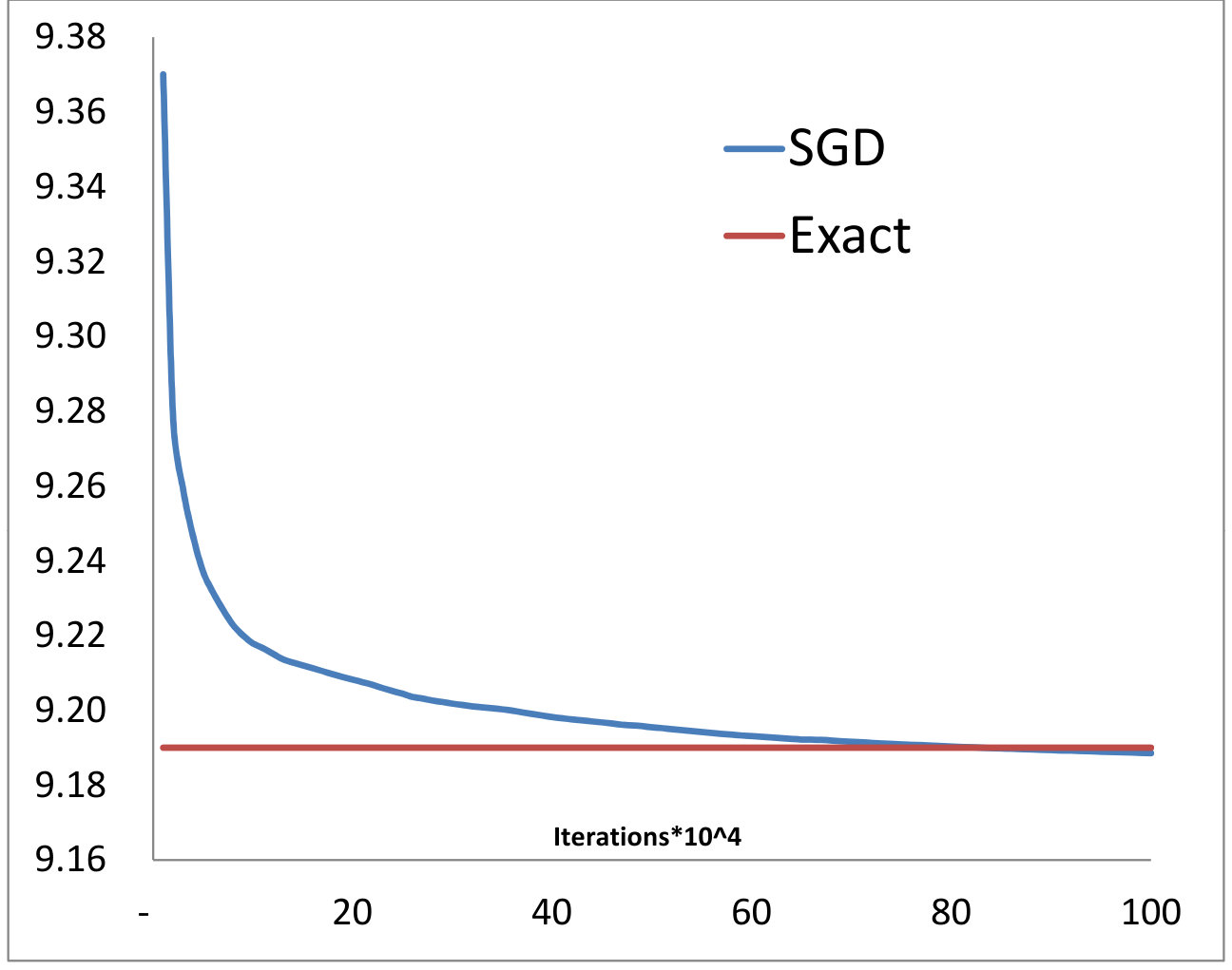 Figure 1
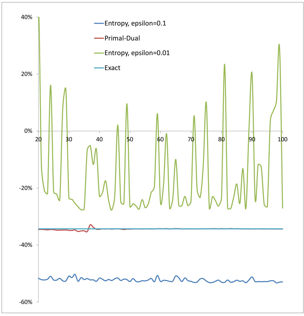 Figure 2
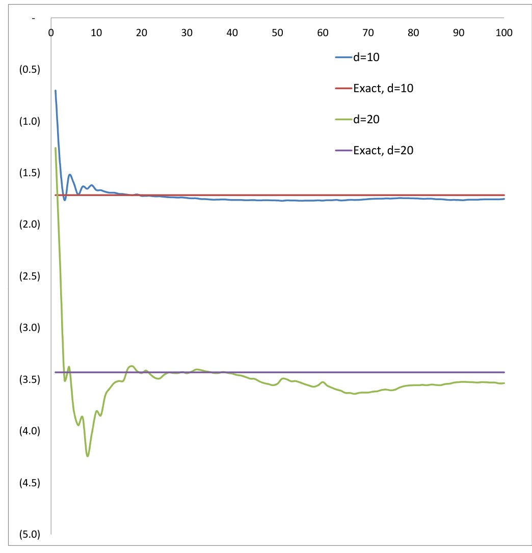 Figure 3
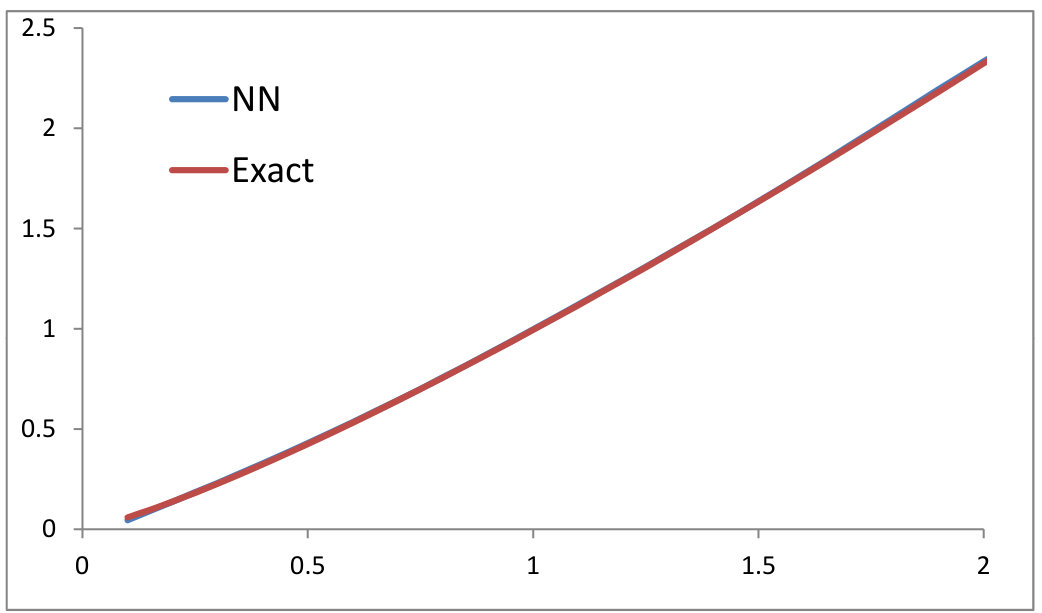 Figure 4
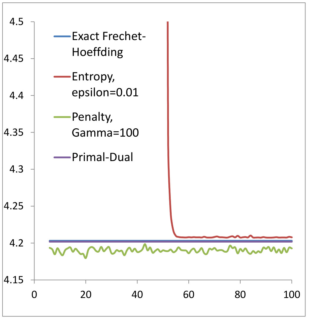 Figure 5
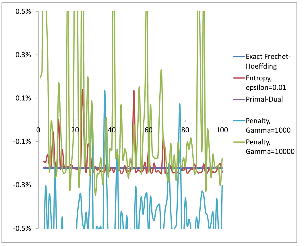 Figure 6
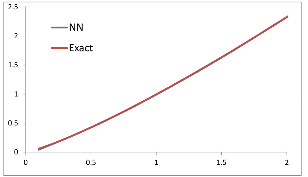 Figure 7
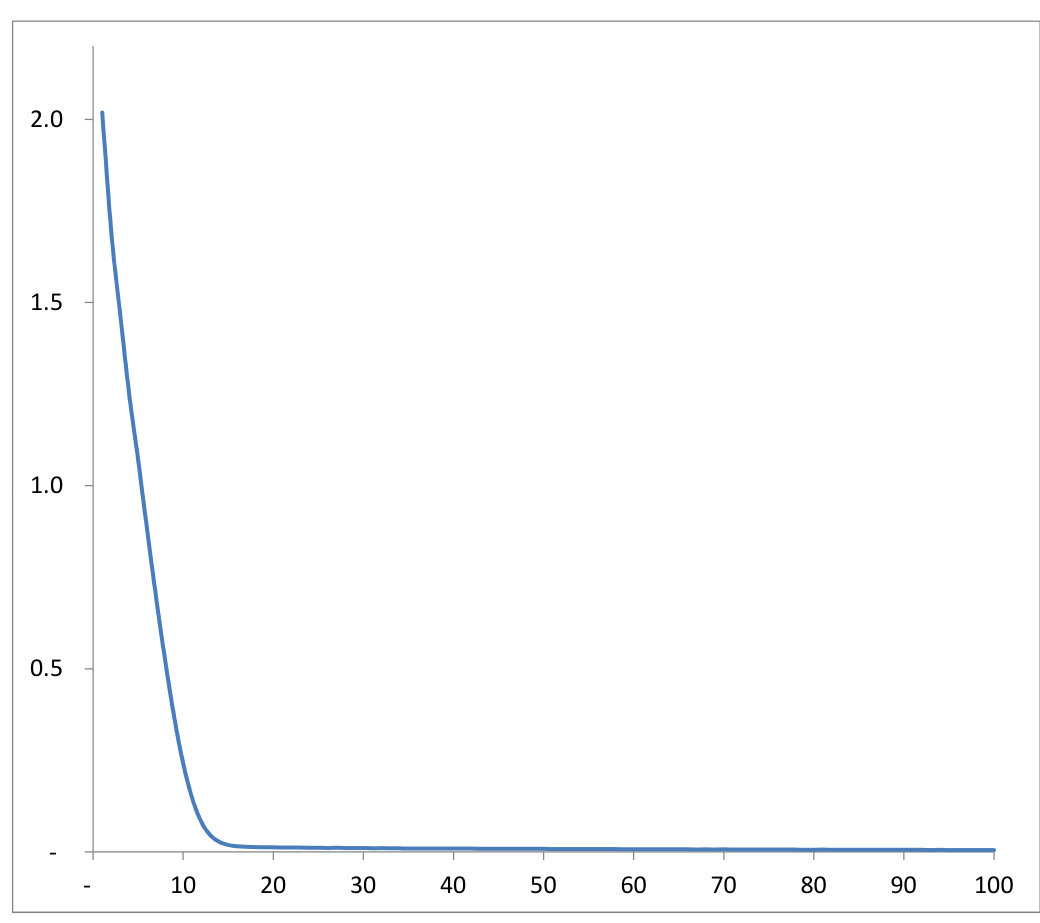 Figure 8
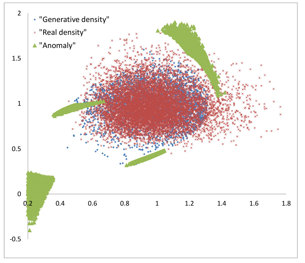 Figure 9
Peer Reviews
No public reviews on file for this paper yet. If you reviewed it on a platform where reviews are public (OpenReview, ICLR, NeurIPS, ICML), you can paste yours below so the community can read it here.
Videos
No videos yet. Explain this paper in a talk, walkthrough, or lecture? Add one.
(Martingale) Optimal Transport and anomaly detection with neural networks: a primal-dual algorithm
Pierre Henry-Labordère
Société Générale, Global markets Quantitative Research
CMAP, Ecole Polytechnique
Abstract.
In this paper, we introduce a primal-dual algorithm for solving (martingale) optimal transportation problems, with cost functions satisfying the twist condition, close to the one that has been used recently for training generative adversarial networks. As some additional applications, we consider anomaly detection and automatic generation of financial data.
Key words and phrases:
(Martingale) optimal transport, Arrow-Hurwicz’s algorithm, generative adversarial networks, anomaly detection
1. Introduction
We introduce a primal-dual algorithm for solving (martingale) optimal transportation problem (in short MOT), potentially large-scale, using neural networks. The martingale optimal transport, first introduced in [2] and in a continuous-time setting in [11], can be defined in a discrete-time setting as the following infinite-dimensional linear program:
[TABLE]
where is a weak compact convex set and is the set of probability measures on (or if the random variables and are interpreted as financial asset prices). A similar definition applies by replacing the supremum over by an infimum. is a number which depends on a cost function and two marginal distributions and defined on . In comparison with the classical OT, we have an additional martingale constraint and the linear problem is well-posed if and only if in the convex order. In mathematical finance, can then be interpreted as the model-independent arbitrage-free optimal upper bound for a payoff depending on an asset evaluated at two maturities , i.e., , , which is consistent with the prices (at ) of and (-dimensional) European basket options (see [15] for an extensive introduction to MOT and its relevance in arbitrage-free pricing). Our algorithm, described in Section 3, can also be applied to more general linear programs of the form:
[TABLE]
where is a weak-compact convex subset of , see for example the multi-marginals (M)OT. However, our algorithm will be applicable only to cost functions satisfying a (martingale) twist condition. Although the extension of our algorithm to this more general setting is straightforward, we prefer for the sake of simplicity to focus on (martingale) OT as defined by (1). Most of the numerical schemes of (M)OT, that we will describe, rely strongly on the dual Monge-Kantorovich formulation in which can be written as (see [2] for a proof in the context of MOT):
[TABLE]
such that for all
[TABLE]
By definition, .
2. Numerical algorithms: A short overview
In this section, we review three numerical algorithms for solving (martingale) optimal transport and highlight their main drawbacks111We acknowledge G. Peyré for useful discussions.. These algorithms will be compared to our primal-dual method in Section 4.
2.1. Simplex and cutting-plane
The problem (2) (resp. 1) defines a linear program that can be solved using a simplex algorithm. In the context of MOT, this has been explored in [16]. By discretizing the measures and on a large grid in , we obtain a finite-dimensional linear program. Due to the large number of linear constraints (3), one can use a cutting-plane algorithm, see [16] for extensive details. This consists in solving the LP program using first a small dimensional grid (). The optimal bound is attained by the dual variables . Then we check on the full grid if our optimal dual solution violates the linear constraints (3). The points of where the linear constraints are not satisfied, are then added to the grid , defining a new refined grid . By construction, we obtain as . The procedure is then iterated until the optimal dual solution at step satisfies all the constraints on for which we can conclude that we have converged towards the true solution. Despite its simplicity, this algorithm could not be extended in large dimension as the number of constraints explodes with the dimension. For example, the complexity of the Hungarian/auction algorithms is .
2.2. Entropic relaxation
Another approach is to introduce an entropy penalization (or more generally a -divergence):
[TABLE]
where is the relative entropy with respect to a prior probability measure and is a positive parameter taken to be small. In particular, . The problem can be dualized using the Fenchel-Rockafellar’s theorem into a strictly convex optimization problem [16]:
[TABLE]
2.2.1. Sinkhorn’s algorithm
By computing the gradients with respect to , and , we obtain the first-order optimality conditions:
[TABLE]
For the sake of simplicity, we have assumed here that , and are absolutely-continuous with respect to the Lebesgue measure. The Sinkhorn algorithm can be then described by the following steps:
- (1)
Set and set , , for convenience. We approximate the measures and by Dirac masses supported on points and . 2. (2)
Compute for all using
[TABLE] 3. (3)
Compute for all by finding the (unique) zero of
[TABLE] 4. (4)
Compute for all using
[TABLE] 5. (5)
Set and iterate steps (2-3-4) up to convergence.
The use of the Sinkhorn algorithm for solving OT problem was introduced in [6] and in [14], [7] in the context of MOT (see also [8] for an application to the construction of arbitrage-free implied volatility surfaces). Again this algorithm does not scale well with the dimension as at each Sinkhorn’s iteration, must be computed on a grid whose the cardinality explodes with the dimension . The overall complexity is .
2.3. and neural networks…
In [19], the optimization (4) is solved by approximating the potentials (and ) by some neural networks and then the training is achieved using a stochastic gradient descent algorithm. Similarly, by using Equation (5), the problem (4) can be converted into an equivalent form which involves only the potentials and :
[TABLE]
and solve similarly. In [12], instead of using neural networks, the authors make use of an expansion of the dual variables in a reproducing kernel Hilbert space. Despite this algorithm scales properly with the dimension in practise, we will illustrate in our numerical experiments that our computations are unstable when becomes small. This has been also reported in [12].
2.4. Penalization
In [10], the optimization is approximated by
[TABLE]
where is a large parameter. This ensures that by taking large, the optimal dual solution will satisfy the linear constraints (3) and therefore . As above, the potentials , and are approximated by some neural networks. This is a classical technique for solving linear programs by penalization and in practise the parameter is chosen to increase to a large value as the learning parameter , used in the stochastic gradient descent, decreases. In our numerical experiments, we will illustrate that this algorithm is unstable, when the parameter is chosen large in order to converge to the true solution. Finally, let us remark that the penalization method can be obtained by replacing the entropy penalization by the -divergence .
3. A primal-dual algorithm
3.1. A saddle-point formulation
For the sake of clarity, we explain our algorithm in the case of the classical OT problem which consists in solving
[TABLE]
where . By introducing the Lagrange multipliers and associated to the two marginal constraints, this problem can be written as a minimax (relaxed) optimization problem:
[TABLE]
where denotes the space of positive measures on .
3.2. Using Brenier’s theorem
Definition 3.1** (Twist condition).**
A function differentiable with respect to is said to be twisted if , the map is one-to-one.
We recall the Brenier theorem (see e.g. [20]):
Theorem 3.2** (Brenier’s theorem).**
By assuming that is absolutely continuous with respect to the Lebesgue measure and the cost function satisfies the twist condition, the optimal probability measure , solution of the above saddle-point problem (8), is supported on a unique map :
[TABLE]
Note that the constraints and imply the requirement where denotes the push-forward of the measure by the map . can be characterized as the unique solution of a Monge-Ampère-like equation. More precisely, in the case of the quadratic cost function, is the gradient of a convex function solution of the Monge-Ampère PDE (see e.g. [20]).
Remark 3.3** (Fréchet-Hoeffding ).**
Under the (twist) condition in , the optimal transport can be solved analytically and it is given by the Fréchet-Hoeffding solution:
[TABLE]
The map is then with the cumulative distribution of .
Under the twist condition, the above minimax optimization (8) can therefore be simplified as
[TABLE]
Note that as , the potential has disappeared and the minimax optimization involves now only the potential and the Brenier map .
3.3. and neural networks…
We then approximate the two unknowns and with two neural networks depending respectively on some weights and . can then be approximated by
[TABLE]
In particular, from the universal approximation property of neural networks, we have .
3.4. Link with Wasserstein generative adversarial networks
The -Wasserstein distance corresponds to an OT problem with a -cost in , :
[TABLE]
defines then a distance which metrizes the space (see e.g. [20]). If we consider a probability measure in corresponding to some real data, one would like to reconstruct this density using a mapping with and such that the push-forward of by a prior density supported on (e.g. an uniform or Gaussian density for the sake of simplicity) is as close as possible to with respect to the Wasserstein distance. The mapping is then chosen to be the solution of
[TABLE]
Note that and this is why it is not possible to use the relative entropy as in the case of maximum likelihood estimation. Using the saddle-point formulation of the Wassertein distance (the -cost satisfies the twist condition) explained in the previous section, this is equivalent to the following minimax optimization:
[TABLE]
This problem is similar to (10) and therefore as described in Section 3.6, our algorithm is close in spirit to the one used for training Wasserstein generative adversarial networks [1] (see also [13]).
Specializing to , we get
[TABLE]
This should be compared with the dual formulation of the -Wassertein distance used in [1]
[TABLE]
where the supremum is over all the -Lipschitz functions. The Lipschitz constraint is enforced in brute force by weight clipping.
Starting from the primal formula of OT and using the Brenier theorem, can also be written as
[TABLE]
This was done in [4] although the Brenier result is not mentioned. The constraint is then implemented by adding a penalty term with large:
[TABLE]
One obtains the Wasserstein-VAE formulation.
3.5. Anomaly detector and data generator
Let us consider some real data generated by a density and let us choose a prior density supported on a low-dimensional manifold. As outlined above, we find the density such that the -Wasserstein distance is minimized. Then, a data will be considered as an anomaly if is below a certain threshold :
[TABLE]
Similarly, a new data can be generated by drawing a random variable distributed according to and set .
3.6. Arrow-Hurwicz algorithm: recipe
We simulate and by Monte-Carlo with paths and for large , our optimization (11) consists in solving:
[TABLE]
where
[TABLE]
The average functional can be optimized by using a stochastic Arrow-Hurwicz algorithm which consists in doing sequentially the two iterations at each step : Draw a uniform r.v. and compute
[TABLE]
where is a learning parameter. In practise, the gradients are computed by back-propagation where
[TABLE]
We could used also a predictor-corrector scheme (that gives similar results in our numerical experiments):
[TABLE]
3.7. Convergence
By using one layer for the approximation of the two unknowns and with a linear activation function (a drift can also be included without loss of generality):
[TABLE]
the problem (11) can be written as
[TABLE]
and it is of the form
[TABLE]
where is a linear operator. As shown by [5], the stochastic Arrow-Hurwicz algorithm converges if is concave, is convex and . Our program (14) is clearly convex in as being linear and is concave in if and only if . This implies that our algorithm converges (in the case of one layer), if we impose that . Additionally, we should have that satisfies the twist condition as we have used the Brenier theorem.
Let us remark that if we consider the new cost function , then we have for all :
[TABLE]
Using this property, we can apply our algorithm to the cost function where is chosen such that222We are grateful to our master-degree students Y. Chen and F. Jiang at Ecole Polytechnique for pointing to us this remark.
[TABLE]
Example 3.4**.**
For , we can take . For , we can take .
Using the result in [5], we conclude:
Proposition 3.5** (Convergence).**
Let us assume that satisfies the twist condition and for some twice differentiable function in , then the Arrow-Hurwicz algorithm (with one layer) (12-13) converges for small enough.
Note that a similar conclusion appears if we expand and in terms of a reproducing kernel Hilbert space.
3.8. The case of MOT
For , under the (martingale) twist condition , the optimal probability measure is shown to be supported not on a single map but on two maps [3, 17]:
[TABLE]
This leads to the following minimax optimization:
[TABLE]
Note that the martingale condition leads explicitly to but we do not use this equation in order to preserve the concavity-convexity property with respect to the neural network weights (in the case of one layer). The algorithm is then similar to the one presented for OT except that now we have five (instead of two) neural networks for the potentials and the two maps and .
For , one can characterize the cost functions for which the optimal probability measure is supported on maps [9]. The above optimization becomes therefore:
[TABLE]
where . In practise, the number of maps can be seen as an hyperparameter that can be optimized.
4. Numerical examples
4.1. OT in
We first check our algorithm described in Section 3.6 for OT problem in . We consider the two cost functions and satisfying the conditions in Proposition 3.5 (see Figures 1 and 2). and are chosen to be two log-normal distributions in centered at and with variances and . They are simulated using Monte-Carlo paths. For each neural network, we have used hidden layers of dimension . We have also used a Adam stochastic gradient descent [18] with minibatches for the computation of the online gradients and our algorithm has been written from crash in C++. The exact solution has been computed using formula (9) and performing a 1d numerical integration. We have compared our algorithm with the entropy relaxation and the penalization methods outlined in Sections 2.2-2.4. We can observe that our primal-dual algorithm converges faster (to the exact solution). On one hand, the choice of the gamma factor in the penalization method is tricky. Taking a small value of results into convergence towards a false solution and a large gives noisy results. On the other hand, the entropy relaxation needs more iterations to converge. We have used in all our numerical experiments at most iterations. For each iterations where ranges from up to , we have computed the functional by averaging over our recorded Monte-Carlo paths. We have also plotted the map found by our algorithm (denoted “NN”) and compared with the Fréchet-Hoeffding solution . We found a perfect match (the blue and red curves coincide).
4.2. -Wassertein distance in ,
Next, we compute the -Wassertein distance in . In our notation, this corresponds to the payoff with a minus sign. We have first considered (see Figure 3–left). We have compared the entropy relaxation method against our primal-dual algorithm. As concluded in , our algorithm converges faster and the entropy relaxation method is unstable according to our choice of . For large epsilon, the Wasserstein distance is underestimated and for small epsilon, our SGD is noisy and therefore the result can not be trusted. As a consequence, the entropy relaxation method could not be used as presented for computing the Wasserstein distance. The convergence is very fast for our primal-dual method. Here and are chosen to be two uncorrelated normal distributions in with variances and for which the exact -Wassertein distance in is . Then, we consider only our primal-dual algorithm and take and (see Figure 3–right). For each neural network, we have used hidden layer of dimension .
4.3. MOT in
A similar test has been performed in the case of MOT in with a cost for which the martingale twist condition is satisfied. Our optimization converges towards the exact solution obtained using a simplex algorithm (see Figure 4).
4.4. Anomaly detection in
As a final simple numerical example, we consider our anomaly detection algorithm outlined in Section 3.5. We have used hidden layers of dimension with linear activation output. We take for a two-dimensional uncorrelated log-normal distribution with mean , variance and for a two-dimensional uncorrelated normal distribution. They are simulated using Monte-Carlo paths. Note that the stochastic Arrow-Hurwicz iterations over and are performed and each iterations, a stochastic gradient descent minimization over is done. We have plotted in Figure 5 the -Wasserstein distance each iterations and this converges, as expected, to zero. Once the mapping is constructed by optimization, we generate some “anomalies” by drawing some normal variables in and adding an anomaly factor . The “normal” variables are generated without introducing this anomaly factor. The two-dimensional “normal” and “abnormal” variables generated are then displayed in Figure 6. As expected, the “abnormal” data live on the edge of the two-dimensional uncorrelated log-normal distribution , which is close to with respect to the -Wasserstein distance (see Figure 5).
The reference list from the paper itself. Each links out to its DOI / PubMed record.
- 1[1] Arjovsky, M., Chintala, S., Bottou, L. : Wasserstein GAN , ar Xiv:1701.07875.
- 2[2] Beiglböck, M., Henry-Labordère, P., Penkner, F. : Model-independent Bounds for Option Prices: A Mass-Transport Approach , Finance and Stochastics, July 2013, Volume 17, Issue 3, pp 477–501.
- 3[3] Beiglböck, M., Juillet, N. : On a problem of optimal transport under marginal martingale constraints , Ann. Probab. Volume 44, Number 1 (2016), 42-106.
- 4[4] Bousquet, O., Gelly, S., Tolstikhin, I., Simon-Gabriel, C-J, Schölkopf, B. : From Optimal Transport to Generative Modeling: the VEGAN cookbook , ar Xiv:1705.07642.
- 5[5] Chambolle, A., Pock, T. : A first-order primal-dual algorithm for convex problems with applications to imaging , Journal of Mathematical Imaging and Vision, 2011.
- 6[6] Cuturi, M. : Sinkhorn Distances: Lightspeed Computation of Optimal Transportation Distances , Advances in Neural Information Processing Systems 26, pages 2292–2300, 201.
- 7[7] De March, A. : Entropic resolution for multi-dimensional optimal transport , arxiv:181211104.
- 8[8] De March, A., Henry-Labordère, P. : Building arbitrage-free implied volatility: Sinkhorn’s algorithm and variants , ar Xiv:1902.04456.