A multi-lane macroscopic traffic flow model for simple networks
Paola Goatin (Acumes), Elena Rossi (Acumes)

TL;DR
This paper develops a well-posed macroscopic traffic flow model for multi-lane networks, accommodating real-world complexities like lane changes and speed discontinuities, supported by mathematical proofs and numerical simulations.
Contribution
It introduces a novel multi-lane traffic model with space discontinuities and proves its well-posedness, extending previous models to more realistic scenarios.
Findings
Existence of solutions established via compactness of Godunov's approximations.
L^1-stability demonstrated using the doubling of variables technique.
Numerical simulations illustrate the model's behavior in sample cases.
Abstract
We prove the well-posedness of a system of balance laws inspired by [8], describing macro-scopically the traffic flow on a multi-lane road network. Motivated by real applications, we allow for the the presence of space discontinuities both in the speed law and in the number of lanes. This allows to describe a number of realistic situations. Existence of solutions follows from compactness results on a sequence of Godunov's approximations, while -stability is obtained by the doubling of variables technique. Some numerical simulations illustrate the behaviour of solutions in sample cases.
Click any figure to enlarge with its caption.
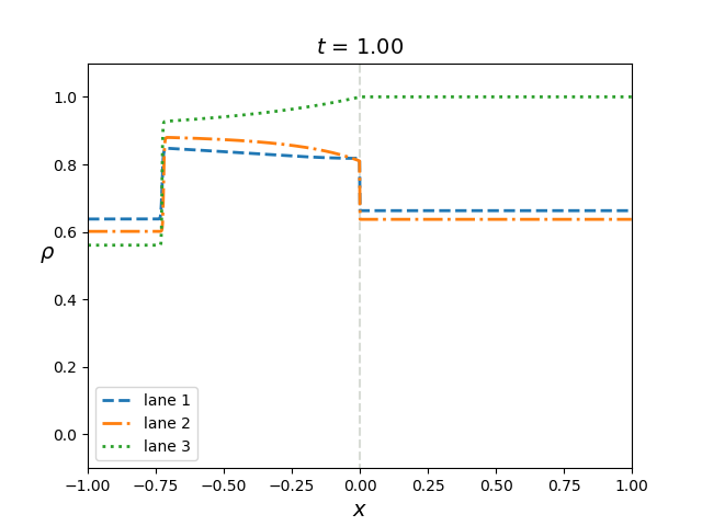 Figure 1
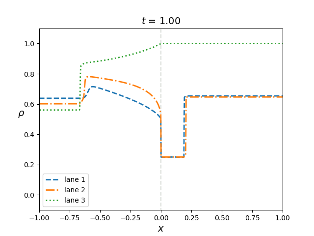 Figure 2
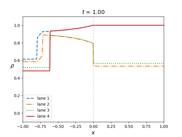 Figure 3
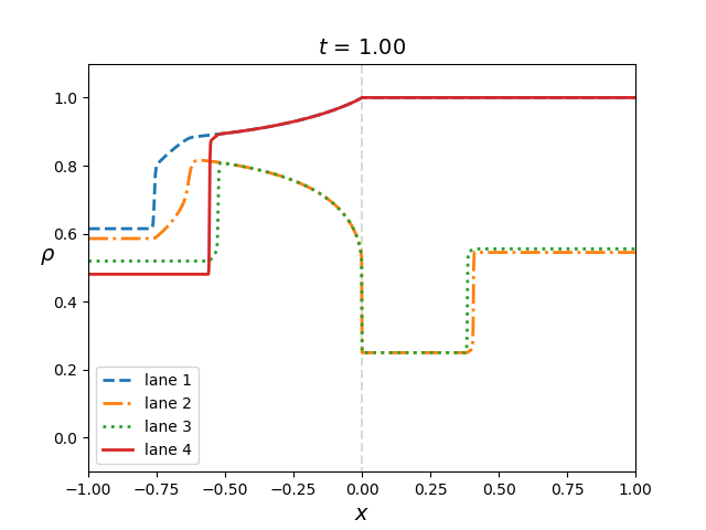 Figure 4
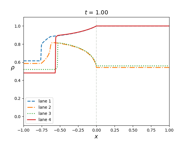 Figure 5
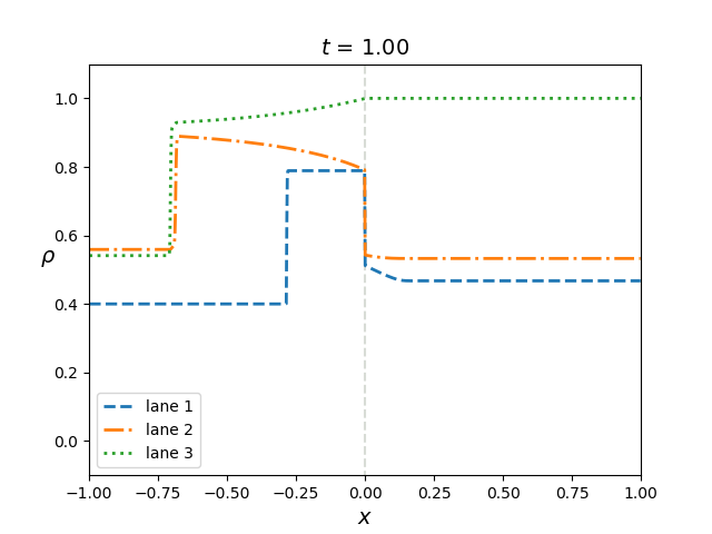 Figure 6
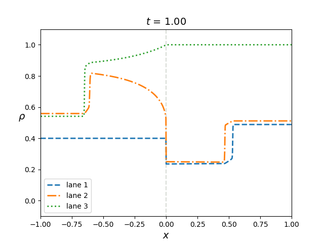 Figure 7
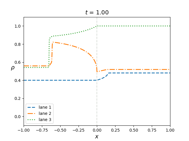 Figure 8
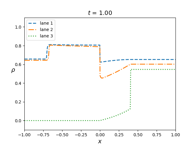 Figure 9
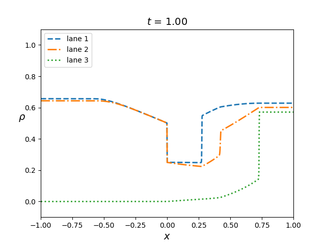 Figure 10
Peer Reviews
No public reviews on file for this paper yet. If you reviewed it on a platform where reviews are public (OpenReview, ICLR, NeurIPS, ICML), you can paste yours below so the community can read it here.
Videos
No videos yet. Explain this paper in a talk, walkthrough, or lecture? Add one.
A multi-lane macroscopic traffic flow model for simple networks
Paola Goatin111Inria Sophia Antipolis - Méditerranée, Université Côte d’Azur, Inria, CNRS, LJAD, 2004 route des Lucioles - BP 93, 06902 Sophia Antipolis Cedex, France. E-mail: {paola.goatin, elena.rossi}@inria.fr
Elena Rossi111Inria Sophia Antipolis - Méditerranée, Université Côte d’Azur, Inria, CNRS, LJAD, 2004 route des Lucioles - BP 93, 06902 Sophia Antipolis Cedex, France. E-mail: {paola.goatin, elena.rossi}@inria.fr
Abstract
We prove the well-posedness of a system of balance laws inspired by [8], describing macroscopically the traffic flow on a multi-lane road network. Motivated by real applications, we allow for the the presence of space discontinuities both in the speed law and in the number of lanes. This allows to describe a number of realistic situations. Existence of solutions follows from compactness results on a sequence of Godunov’s approximations, while -stability is obtained by the doubling of variables technique. Some numerical simulations illustrate the behaviour of solutions in sample cases.
2010 Mathematics Subject Classification: 35L65, 90B20, 82B21.
Keywords: macroscopic multi-lane traffic flow model on networks; Godunov scheme; well-posedness.
1 Introduction
Macroscopic traffic flow models consisting of hyperbolic balance laws have been developed in the scientific literature starting from the celebrated Lighthill-Whitham-Richards (LWR) model [13, 14]. Despite its simplicity, the LWR model is able to capture the basic features of road traffic dynamics, such as congestion formation and propagation. Nevertheless, it cannot describe many aspects of road traffic complexity. To this end, several improved models accounting for specific flow characteristics have subsequently been introduced: second-order models accounting for a momentum equation (see e.g. [2]), multi-population models distinguishing between different classes of vehicles (e.g. [3]), etc.
In this paper, we are interested in describing carefully the traffic dynamics on road networks with several lanes, allowing for lane change and overtaking. Multi-lane models for vehicular traffic have been proposed in [6, 8, 11, 12]. In the macroscopic setting, these models consist in a system of balance laws in which the transport is expressed by a LWR equation for each lane, and the source term accounts for the lane change rate. In particular, the equations of the system are coupled in the source term only.
Aiming to describe realistic situations in detail, we allow for the speed laws and the number of lane to change along the road. In the study, for sake of simplicity, we consider the model proposed in [8], but more general source terms could be taken into account.
We consider an infinite road described by the real line. Let be the set of indexes of the active lanes on , with its cardinality, and be the set of indexes of the active lanes on , with . Let us consider , its choice depending on the specific situation under study.
To cast the problem in a general setting, we extend the road considering the same number of lanes on the left and on the right of . More precisely, we assume that there are and additional empty lanes on , respectively . Moreover, we prevent vehicles from passing from the active to the fictive lanes added, see condition (1.9) below. In the same way, we can consider multiple separate roads, thus accounting for network nodes.
The problem under consideration is then the following: for and , the vehicle density on lane solves the Cauchy problem
[TABLE]
with
[TABLE]
for , where is the Heaviside function. The velocities , for and , are strictly decreasing positive functions such that . We assume that each map admits a unique global maximum in the interval , attained at . We set
[TABLE]
Moreover, we set for and
[TABLE]
Concerning the source terms, accounting for the flow rate across lanes, we define, as in [8],
[TABLE]
for and , where and . To account for separate lanes, such as different roads or fictive lanes, we set
[TABLE]
The functions appearing in the source term are then defined as follows
[TABLE]
For the sake of shortness, introduce the notation , so that the initial data associated to problem (1.1)–(1.6)–(1.7) read .
Remark 1.1**.**
For simplicity, and with slight abuse of notation, we consider for , . However, we will show that, by (1.6), (1.7) and (1.9), there holds for all , and , respectively for all , and .
Following [10, Definition 5.1], see also [9, Definition 2.1 and Formula (5.8)] and [7, § 8.3], we recall the definition of weak entropy solution for (1.1)–(1.6)–(1.7).
Definition 1.2**.**
A map is a weak entropy solution to the initial value problem (1.1) if
for any and for all ,
[TABLE] 2. 2.
for any , for any and for all
[TABLE]
The rest of the paper is organised as follows. In Section 2 we construct a sequence of approximate solutions based on Godunov finite volume scheme and we prove its convergence towards a solution of (1.1). We then provide a -stability estimate with respect to the initial data, which implies the uniqueness of solutions. Specific situations and the corresponding numerical simulations are discussed in Section 3.
2 Well-posedness
We define the map by setting and , for . Moreover we define
[TABLE]
We introduce the following quantity, which corresponds to the –norm of the vector computed on active lanes:
[TABLE]
Introduce a uniform space mesh of width and a time step , subject to a CFL condition, to be detailed later on. For set
[TABLE]
where denotes the centre of the cell, while its interfaces. Observe that corresponds to , so that non negative integers denote the cells on the positive part of the -axis. Set and let , for , be the time mesh. Set . Approximate the initial data in the following way: for , for
[TABLE]
Define a piece-wise constant solution to (1.1) as, for ,
[TABLE]
through a Godunov type scheme (see [1]) together with operator splitting, to account for the source terms:
Algorithm 2.1**.**
[TABLE]
Remark 2.2**.**
*Observe that, under hypotheses (1.6)–(1.7), for all and (corresponding to ), it holds for all . In particular, no wave can move backward into the segment for . Similarly, for all and (corresponding to ), it holds for all . In particular, no wave can move forward into the segment for . *
2.1 Positivity and upper bound
We prove that, under a suitable CFL condition, if the initial data take values in the interval , then also the approximate solution constructed via Algorithm 2.1 attains values in the same interval .
Lemma 2.3**.**
Let . Assume that
[TABLE]
with as in (2.1). Then, for all and , the piece-wise constant approximate solution constructed through Algorithm 2.1 is such that , for all .
Proof. By induction, assume that for all and . Consider (2.7): it is well known that, for a Godunov type scheme with discontinuous flux function, it holds , see [1, Lemma 4.3]. We now focus on the remaining step, involving the source term. In particular, fix , corresponding to , the other case being entirely similar. Exploiting (1.10), equation (2.8) reads
[TABLE]
To improve readability, in what follows we omit the index . Moreover, we take into account a complete case, in which the source term contains the contributions from both the previous and the subsequent lane. Without loss of generality, we take and we assume both and . By (2.8) and (1.8) we obtain
[TABLE]
There are four possibilities:
[TABLE]
We analyse them in details.
- A.
Equation (2.10) reads
[TABLE]
by the CFL condition (2.9), since . Moreover, since and ,
[TABLE]
with and we exploit the fact that , due to the CFL condition (2.9). 2. B.
By equation (2.10) and the hypotheses on the signs, it follows immediately that
[TABLE]
Moreover, since and , we get
[TABLE]
where . 3. C.
By equation (2.10) and the hypotheses on the sign, we get
[TABLE]
by the CFL condition (2.9), since . Moreover, since and , we get
[TABLE] 4. D.
By equation (2.10) and the CFL condition (2.9) we obtain
[TABLE]
Moreover, since and ,
[TABLE]
where .
Hence, we conclude that for all and .
2.2 –bound
The following Lemma shows that, if the initial datum satisfies , i.e. it is in on the active lanes, the same holds for the corresponding solution. Moreover, the –norm (2.2) is constant, thus the total number of vehicles is preserved over time.
Lemma 2.4**.**
Let . Let , with . Under the CFL condition (2.9), the piece-wise approximate solution constructed through Algorithm 2.1 is such that, for all ,
[TABLE]
Proof. By induction, assume that (2.11) holds for . The Godunov type scheme (2.7) is conservative, see [1], hence
[TABLE]
Pass now to (2.8): by the positivity of , see Lemma 2.3, and the assumptions on the source terms (1.11), it follows immediately that .
2.3 continuity in time
Following the idea introduced in [9, Lemma 3.3], we now prove the -continuity in time of the numerical approximation, constructed through Algorithm 2.1. The result is of key importance in the subsequent analysis.
Proposition 2.5**.**
Let with . Assume that the CFL condition (2.9) holds. Then, for
[TABLE]
with and as in (2.1).
Remark 2.6**.**
Observe that, by Remark 2.2, the sums appearing in (2.12) are actually sums over the active lanes only, the terms corresponding to fictive lanes being equal to 0. For example
[TABLE]
However, for the sake of shortness, we keep the first notation throughout the proof.
Proof. Fix and . By (2.8) we have:
[TABLE]
Observe that, by (1.11), terms of type are non zero for . For and , the function defined in (1.10), together with (1.8) and (1.9), is Lipschitz in both variables, with Lipschitz constant
[TABLE]
with as in (2.1). Hence, for , we get
[TABLE]
By (2.13), taking into account also (1.11), we conclude
[TABLE]
Exploit now (2.7): we have, for fixed and ,
[TABLE]
We closely follow the proof of [9, Lemma 3.3]. In (2.15) add and subtract and and, setting
[TABLE]
rearrange the resulting expression to obtain
[TABLE]
Since the numerical flux defined in (2.6) is non decreasing in the second variable and non increasing in the third, we get for all and . Moreover, is Lipschitz in both arguments, for , with Lipschitz constant bounded by as in (2.1). Therefore,
[TABLE]
by the CFL condition (2.9). A similar argument applies to . As a consequence, , thus all the coefficients appearing in (2.22) are positive and so
[TABLE]
Collecting together (2.14) and (2.23) leads to
[TABLE]
which applied recursively yields
[TABLE]
where we also multiplied both sides of the inequality by .
Using (2.7) and (2.8), compute
[TABLE]
Focus first on (2.26): by the definition of (1.8)–(1.10)–(1.11), for we have
[TABLE]
Therefore, recalling Remark 2.6, with slight abuse of notation
[TABLE]
where we use Lemma 2.4.
Pass now to (2.25). Since we are interested in the sum over , we distinguish among four cases: , , and .
The first case, , amounts to . Thus, by the definition of (2.6), together with (1.4), the numerical flux does not depend on the variable , namely
[TABLE]
and the function above is clearly Lipschitz in both and , with Lipschitz constant as in (2.1), leading to
[TABLE]
The case can be treated analogously, leading to
[TABLE]
Pass now to . Recall that . By the definition of (2.6), together with (1.4), we have
[TABLE]
We immediately get
[TABLE]
with as in (2.1). The case follows analogously.
Hence, collecting together (2.29), (2.30) and (2.31) and using the fact that , we obtain
[TABLE]
By (2.25)–(2.26), insert (2.28) and (2.32) into (2.24):
[TABLE]
concluding the proof.
2.4 Spatial bound
We follow the idea of [4, Lemma 4.2] of providing a local spatial bound, in the sense that the estimate in (2.33) below blows up if one of the endpoints of the interval approaches .
Lemma 2.7**.**
*Let with . Assume that the CFL condition (2.9) holds. For any interval such that , fix such that and . Then, for any the following estimate holds: *
[TABLE]
with , and as in (2.1) and independent of and .
Proof. Let
[TABLE]
By the assumptions on , observe that there are at least 2 elements in each of the sets above, i.e. . Moreover, and . Furthermore, notice that
- •
if : it holds for any ;
- •
if : it holds for any .
By Proposition 2.5, there exists a constant such that
[TABLE]
with . Hence, when restricting the sum over in the set , respectively , it clearly follows that
[TABLE]
Choose and with such that
[TABLE]
Thus, by (2.34),
[TABLE]
In view of the next steps, observe that
[TABLE]
Focus on the central sum on the right hand side of (2.36). By (2.8), for and , we have
[TABLE]
By the Lipschitz continuity of the map for and , we get
[TABLE]
Fix now . Recall that for all either or . Therefore, when applying (2.7), observe that the numerical flux (2.6) is never computed at , leading to
[TABLE]
for , with
[TABLE]
Clearly, it is whenever and whenever . Adding and subtracting into (2.38) and setting
[TABLE]
we can rearrange (2.38) to get
[TABLE]
The function is non decreasing in the first argument and non increasing in the second, so that we easily get . Furthermore, is Lipschitz continuous in both variables, with the same Lipschitz constant (2.1) as : by the CFL condition (2.9)
[TABLE]
and hence . Therefore, for
[TABLE]
We are left with the boundary terms in (2.36). Fix . For , applying first (2.8) then (2.7), in the form of (2.46), we have
[TABLE]
Add and subtract , then take the absolute value and sum over : exploiting (2.27) leads to
[TABLE]
Proceed similarly for :
[TABLE]
Now add and subtract , take the absolute value and sum over :
[TABLE]
By (2.36), collect together (2.37), (2.47), (2.48) and (2.49): since all the coefficients appearing there are positive, we obtain
[TABLE]
where we exploit also Lemma 2.3. Proceeding recursively we finally get, for ,
[TABLE]
where we used also (2.35). Noticing that completes the proof.
2.5 Discrete Entropy Inequality
We follow the idea of [9, Lemma 5.1].
Lemma 2.8**.**
Let with . Assume that the CFL condition (2.9) holds. Then the approximate solution defined by (2.3) through Algorithm 2.1 satisfies the following discrete entropy inequality: for all , for , for and for any
[TABLE]
with
[TABLE]
where , .
Proof. Fix and . Let
[TABLE]
Clearly . Set
[TABLE]
so that . By the properties of the numerical flux , the map is non decreasing in all its arguments. Therefore,
[TABLE]
Sum the two inequalities above: since , observe that
[TABLE]
and
[TABLE]
where we used also (2.8) and the inequality . The thesis immediately follows.
2.6 Convergence
Theorem 2.9**.**
Let with . Let with constant and satisfying the CFL condition (2.9). The sequence of approximate solutions constructed through Algorithm 2.1 converges in to a function such that for . This limit function is a weak entropy solution to problem (1.1)–(1.6)–(1.7) in the sense of Definition 1.2.
Proof. We follow [5, Theorem 5.1] and [9, Theorem 5.1].
Lemma 2.3 ensures that the sequence of approximate solutions is bounded in , in particular , for all , and . Proposition 2.5 proves the -continuity in time of the sequence , while Lemma 2.7 guarantees a bound on the spatial total variation in any interval not containing . Standard compactness results imply that, for any interval not containing , there exists a subsequence, still denoted by , converging in .
Take now a countable set of intervals such that : by a standard diagonal process, we can extract a subsequence, still denoted by , converging in , and almost everywhere in , to a function . Moreover, Proposition 2.5, and in particular formula (2.12), implies that this limit function is such that , with slight abuse of notation concerning the -norm.
It remains to show that the limit function satisfies the integral inequalities in Definition 1.2. Concerning point 1, i.e. the weak formulation, it suffices to apply a Lax-Wendroff-type calculation, similarly to what has been done in [9, Theorem 3.1]. Notice that the presence of the source terms does not add any difficulties in the proof.
As for point 2 in Definition 1.2, i.e. the entropy inequality, we follow [9, Theorem 5.1]. Fix . Let . Multiply the inequality (2.50) by , then sum over and :
[TABLE]
Take into account each term separately. Summing by parts and letting , the Dominated Convergence Theorem yields
[TABLE]
and
[TABLE]
Pass now to (2.53). Observe that, by the definition of the numerical flux (2.6), when it holds , with if and if . Therefore (2.53) gives a contribution only for and :
[TABLE]
A careful analysis of all the possible cases yields
[TABLE]
so that
[TABLE]
Focus now on the last term (2.54): by the Dominated Convergence Theorem
[TABLE]
Collecting together (2.55), (2.56), (2.57) and (2.58) completes the proof.
2.7 -Stability and uniqueness
The following Theorem ensures that the solution to (1.1)–(1.6)–(1.7) depends -Lipschitz continuously on the initial data, thus guaranteeing the uniqueness of solutions.
Theorem 2.10**.**
Let be two weak entropy solutions, in the sense of Definition 1.2, to problem (1.1)–(1.6)–(1.7) with initial data and such that . Then, for a.e. ,
[TABLE]
Remark 2.11**.**
Notice that the sums appearing in (2.59) are actually sums over the active lanes only, the terms corresponding to fictive lanes being equal to [math].
Proof. The idea is to combine together the results contained in [10, § 2 and § 5], in particular [10, Theorem 5.1], and in [5, Theorem 3.1], and then adapt [8, Theorem 3.3].
Indeed, fix . Following [10, Theorem A.1 and Formula (2.22)], it is possible to derive the following inequality for any
[TABLE]
where, for the sake of simplicity, we set
[TABLE]
Inspired by [8, Theorem 3.3], since , respectively , satisfies Point 1 in Definition 1.2, we subtract to the above inequality the equation for and add the equation for , arriving at
[TABLE]
for . Now, we extend the above inequality to . The procedure is similar to that in [10, Theorem 2.1] and it leads to
[TABLE]
for all , where
[TABLE]
Analogously to [10, Theorem 2.1] and [5, Theorem 3.1], it can be proven that . Following again [8, Theorem 3.3] and choosing , for , we get
[TABLE]
It is easy to verify that, for fixed , the map defined in (1.10), together with (1.8), is non decreasing in the second argument and non increasing in the third: setting for the sake of convenience we obtain
[TABLE]
Hence, if we have
[TABLE]
with in the interval between and respectively and as in (2.1). Thus,
[TABLE]
Define
[TABLE]
By (2.63) and (2.64) it follows that
[TABLE]
Gronwall’s inequality then implies that . Therefore, if , i.e. a.e. in and for all , then for , i.e. a.e. in and for all . An application of the Crandall–Tartar Lemma [7, Lemma 2.13] concludes the proof of the –contractivity.
3 Numerical experiments
We present some applications of our result in test cases describing realistic road junction examples. The study is not exhaustive: in particular, specific cases of diverging junctions could be handled adding some information on drivers’ routing preferences upstream the junction. Yet, these situations go beyond the scope of this paper.
In all the numerical experiments, we choose
[TABLE]
thus the maximal speed is the same for all the lanes before, respectively after, . In particular, in each situation we consider two cases, and .
3.1 1-to-1 junction: from 2 to 3 lanes
We consider problem (1.1)–(1.6)–(1.9), with , and .
lane 1lane 2lane 3
The initial data are chosen as follows:
[TABLE]
Moreover, we choose , and or respectively. Figure 1 displays the solutions in both cases at time : on the right the maximal speed decreases, on the left it is increasing. We notice the effect of the flow between neighbouring lanes: all along the -axis vehicles moves from lane 1 to lane 2, for vehicles pass also from lane 2 to lane 3, and this is particularly evident near .
3.2 1-to-1 junction: from 3 to 2 lanes
We consider problem (1.1)–(1.7)–(1.9), with , and .
lane 1lane 2lane 3
The initial data are chosen as follows:
[TABLE]
We choose , and or respectively. Figure 2 displays the solutions in both cases at time : on the right the maximal speed decreases, on the left it is increasing. We display the solution also for the positive part of the third lane: it is constantly equal to the maximal density . As in the case of an increasing number of lanes, we notice the effect of the flow between neighbouring lanes. Observe that no vehicle passes from lane 3 to lane 2 for : indeed, lane 3 for is a fictive lane and we impose (1.9) ().
Focus on the queue forming before and compare the two cases, and . When the maximal speed diminishes, the queue is longer and the number of vehicles in the queue is greater with respect to the case of increasing maximal speed: for , in the former case it is more difficult for vehicles in lane 3 to pass in lane 2, since here the decrease in the maximal speed diminishes the flow at .
3.3 2-to-1 junction : from 3 to 2 lanes
We consider the same setting of Section 3.2, thus problem (1.1)–(1.7)–(1.9), with , and initial data (3.2), with the additional assumption that there is no flow of vehicles between the first and the second lane on , i.e. (we keep ):
lane 1lane 2lane 3
We choose and . Figure 3 displays the solution in the three cases at time : on the right the maximal speed decreases, in the centre it stays constant, on the left it increases. As before, we display the solution also for the positive part of the third lane, where it is constantly equal to .
3.4 2-to-1 junction: from 4 to 2 lanes
We consider the problem (1.1)–(1.7)–(1.9), with , and initial data
[TABLE]
with the additional assumption that there is no flow of vehicles between the second and the third lane on , i.e. (we also impose ). The situation under consideration looks as follows:
lane 2lane 3lane 1lane 4
We choose and . Figure 4 displays the solution in the three cases at time : on the right the maximal speed decreases, in the centre it stays constant, on the left it increases. As before, we display the solution also for the positive part of the first and fourth lane, where it is constantly .
Acknowledgement: The authors are grateful to Rinaldo M. Colombo for stimulating discussions.
The reference list from the paper itself. Each links out to its DOI / PubMed record.
- 1[1] Adimurthi, J. Jaffré, and G. D. Veerappa Gowda. Godunov-type methods for conservation laws with a flux function discontinuous in space. SIAM J. Numer. Anal. , 42(1):179–208, 2004.
- 2[2] A. Aw and M. Rascle. Resurrection of “second order” models of traffic flow. SIAM J. Appl. Math. , 60(3):916–938, 2000.
- 3[3] S. Benzoni-Gavage and R. M. Colombo. An n 𝑛 n -populations model for traffic flow. European J. Appl. Math. , 14(5):587–612, 2003.
- 4[4] R. Bürger, A. García, K. H. Karlsen, and J. D. Towers. A family of numerical schemes for kinematic flows with discontinuous flux. J. Engrg. Math. , 60(3-4):387–425, 2008.
- 5[5] R. Bürger, K. H. Karlsen, and J. D. Towers. An Engquist-Osher-type scheme for conservation laws with discontinuous flux adapted to flux connections. SIAM J. Numer. Anal. , 47(3):1684–1712, 2009.
- 6[6] R. M. Colombo and A. Corli. Well posedness for multilane traffic models. Ann. Univ. Ferrara Sez. VII Sci. Mat. , 52(2):291–301, 2006.
- 7[7] H. Holden and N. H. Risebro. Front tracking for hyperbolic conservation laws , volume 152 of Applied Mathematical Sciences . Springer, Heidelberg, second edition, 2015.
- 8[8] H. Holden and N. H. Risebro. Models for dense multilane vehicular traffic. Preprint, 2018.