Phenomenology of SUGRA Extensions of the Starobisnky Model
Ping Kwan Man Ellgan

TL;DR
This paper compares the Born-Infeld (BI) and Starobinsky inflation models, showing they produce similar inflation dynamics under Planck 2018 constraints, and explores parameter scales and inflation signatures.
Contribution
It provides a complete analysis of the BI model, comparing its predictions with the Starobinsky model and examining parameter effects on inflation signatures.
Findings
BI and Starobinsky models have nearly identical inflation dynamics under Planck constraints.
Parameter scales and initial conditions for BI inflation are identified.
Variations in parameters affect the spectral index and tensor-to-scalar ratio.
Abstract
We analyze BI model in a complete form and compare the predictions with that of Starobinsky model. Under the parameter constraints in Planck 2018, we find that the dynamics of the whole inflation process described by BI and Starobinsky models are nearly the same, even though there are some differences in the regions out of inflation. We also find the scales of parameters in BI model and initial inflaton values required to implement inflation. The changes of fingerprints of BI model and that of evolutions of inflaton field due to the variations of relevant parameters are also investigated.
Click any figure to enlarge with its caption.
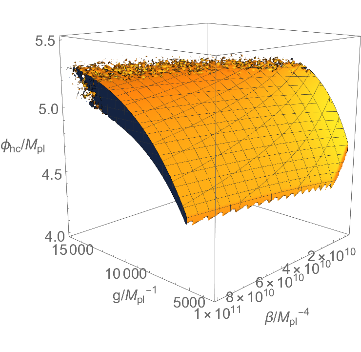 Figure 1
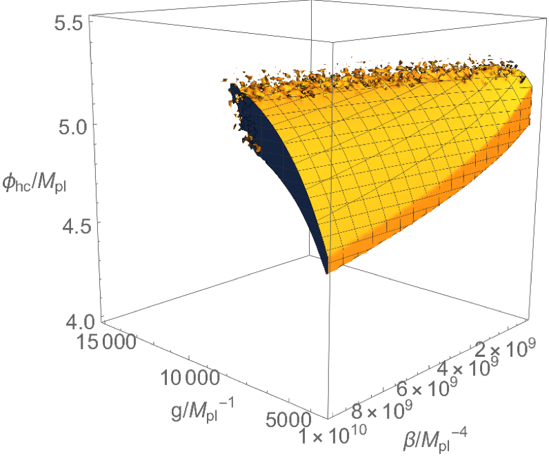 Figure 2
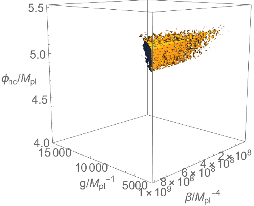 Figure 3
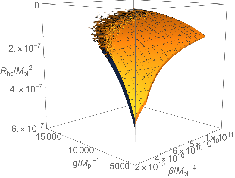 Figure 4
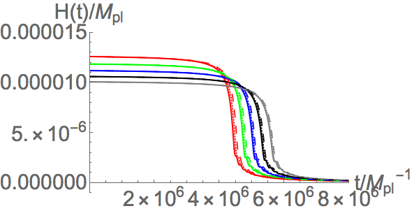 Figure 5
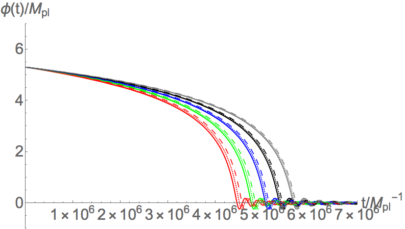 Figure 6
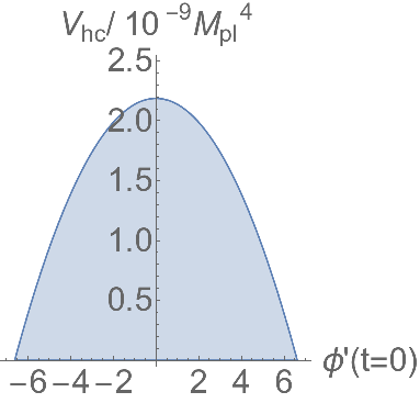 Figure 7
 Figure 8
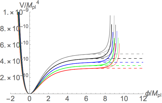 Figure 9
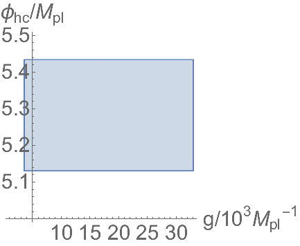 Figure 10
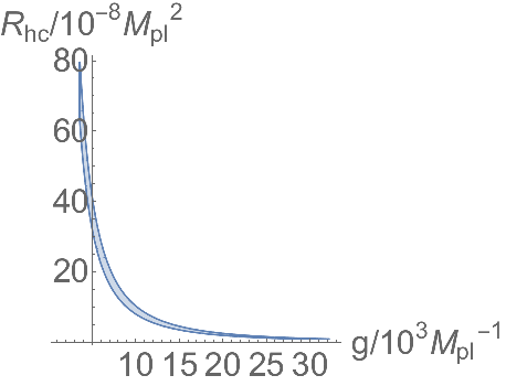 Figure 11
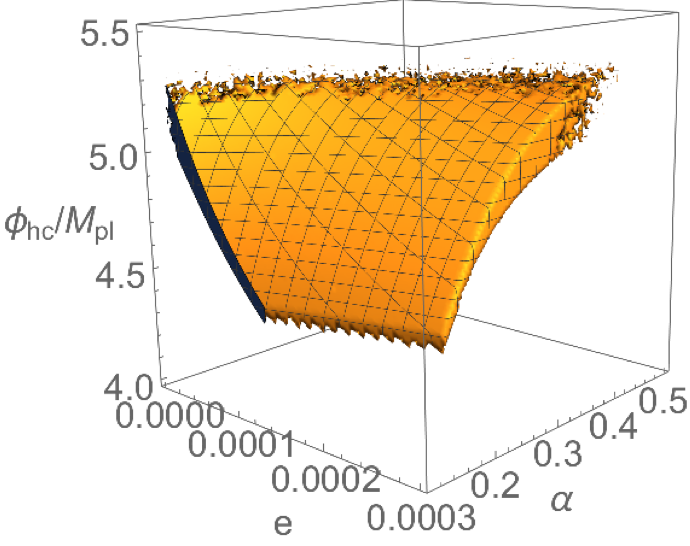 Figure 12
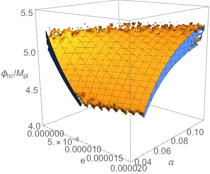 Figure 13
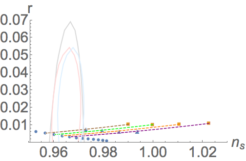 Figure 14
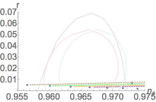 Figure 15
| Slow-roll parameters | Range(s) | Spectral indices | Range(s) |
|---|---|---|---|
| Color, style | Model | ||||
|---|---|---|---|---|---|
| Red, Thick | BI | ||||
| Green, Thick | BI | ||||
| Blue, Thick | BI | ||||
| Black, Thick | BI | ||||
| Gray, Thick | BI | ||||
| Red, Dashed(tiny) | BI | ||||
| Green, Dashed(tiny) | BI | ||||
| Blue, Dashed(tiny) | BI | ||||
| Black, Dashed(tiny) | BI | ||||
| Gray, Dashed(tiny) | BI | ||||
| Red, Dashed(long) | Staro | N/A | |||
| Green, Dashed(long) | Staro | N/A | |||
| Blue, Dashed(long) | Staro | N/A | |||
| Black, Dashed(long) | Staro | N/A | |||
| Gray, Dashed(long) | Staro | N/A |
| Nothing (Gray) | BK14 (Red) | BK14+BAO (Blue) |
| NaN | NaN | |
| NaN | NaN | |
| NaN | NaN | |
| NaN | NaN | |
Peer Reviews
No public reviews on file for this paper yet. If you reviewed it on a platform where reviews are public (OpenReview, ICLR, NeurIPS, ICML), you can paste yours below so the community can read it here.
Videos
No videos yet. Explain this paper in a talk, walkthrough, or lecture? Add one.
Phenomenology of SUGRA Extensions of the Starobisnky Model
00footnotetext: MAN Ping Kwan, Ellgan, E-mail: [email protected]
MAN Ping Kwan, Ellgana)†
1 Abstract
We analyze BI-extended model in a complete form and compare the predictions with that of Starobinsky model. Under the parameter constraints in Planck 2018, we find that the dynamics of the whole inflation process described by BI-extended and Starobinsky models are nearly the same, even though there are some differences in the regions out of inflation. We also find the scales of parameters in BI-extended model and inflaton values at the first horizon crossing required to implement inflation. The changes of fingerprints of BI-extended model and that of evolutions of inflaton field due to the variations of relevant parameters are also investigated.
2 Introduction
Cosmological inflation is a powerful solution to the flatness and horizon problems at the beginning of the standard Big Bang scenario [3, 4, 5]. The constraints of observation data of Planck 2018 are listed in Table 1111Note that in Table 1 is the scalar power spectrum at the first horizon crossing given by
(1)
where is the scalar power spectrum evaluated at the first horizon crossing. . All inflation models naturally provide the primordial density fluctuation and curvature perturbation, which can be observed by cosmic microwave (CMB) background [6, 7]. So far many models listed in [7, 8] can satisfy the observation. In particular, Starobinsky model (also called inflation model), motivated by modified gravity [9, 10], provides the most promising prediction. This triggers many discussions about properties of Starobinsky models during and after inflation like [11] and the counterparts of Starobinsky like models such as [12] and [13], and the dynamics of the extensions of Starobinsky model such as [14] and [15].
On the other hand, it is vital to integrate those inflation models to high energy theories like supergravity (SUGRA). So far, SUGRA, which is a locally supersymmetric theory, has been an appropriate model to unify gravity with particle physics beyond the Standard Model of elementary particles and beyond the Standard Model of cosmology [35]. In particular, the -term potential in SUGRA provides many insights in attractor property, which is describing the connection between Starobinsky model and various power-law model in the graph of tensor-to-scalar ratio against spectral index [16, 17, 18, 19, 20, 21]. Although there is an obstacle called problem resulting from the factor in the -term potential where denotes Kähler potential [22], it was solved by making a proper choice in super-potential and Kähler potential as shown in [23] and [24]. Another solution is discussed in [25] and [26], which considers the scalar component of a massive vector multiplet as an inflaton field. This can avoid the occurrence of problem and realize inflation in a simple way.
It is natural to consider the UV completion of SUGRA inflation models. One possibility is to adopt Dirac-Born-Infeld (DBI) action, which carries zero-mode vector fields attached to the -branes [27, 28]. The supersymmetric (SUSY) version of DBI action was studied in [29] and [30]. The matter coupled DBI type action including a matter charged under symmetry is discussed in [33]. The action of the massive vector multiplet is extended to the DBI type action, which can be constructed by the DBI action of a massless vector multiplet coupled to a Stueckelberg multiplet with symmetry [34], leading to the DBI extension of Starobinsky model and the corresponding dual action222The duality described here is originated from [30]. , with the inflaton field being stored in the lowest scalar component of a massive vector multiplet. This model was also studied in [35], and the effective scales are evaluated under the approximation of the square root term and compared with that of Starobinsky model, with the assumption that the inflaton field is induced from the scalar curvature by the Legendre transformation instead of the scalar field of the massive vector multiplet.
Thus, in this paper, we study the version of [35] in a complete form333We assume the inflaton field is from the scalar curvature instead of the scalar field of the massive vector multiplet. to see how all the higher order terms contribute to the predictions. For the rest of this paper, we call the model we are going to study as "BI-extended model", although there are many meanings for "BI" like "Brane Inflation"[38] and DBI inflation [39]. In section 3, we introduce the basic formalism of obtaining the potential from a general term in a Lagrangian density. After a short review in Starobinsky model in section 4, we analyze the BI-extended model in section 5. In section 6, we show the possible parameters and inflaton values at the first horizon crossing in Starobinsky model and BI-extended model based on the observation constraints listed in Table 1 and how BI-extended model changes as and vary. In section 7, we demonstrate the evolutions of inflaton field as cosmic time runs in different choices of and . Finally, we discuss our results in section 8 and summarize them in section 9.
3 Basic Formalism for studying inflation with model
In this section, we are going to review the basic derivation of 444Note that the mass scale of is , where is the reduced Planck mass. theory555For general review, please refer to [31]. . Note that the Lagrangian is given by
[TABLE]
where is the metric in the Jordan frame666In this paper, notations with a tilde mean the corresponding quantities evaluated in the Jordan frame. . To get the equation of motion (E.O.M.), we vary the action with respect to the metric to produce
[TABLE]
where and is the energy-momentum tensor in the Jordan frame. Also, by taking Legendre Transformation and introducing the new scalar field , we have
[TABLE]
In order to change it from Jordan frame to Einstein frame, we adopt the following conformal transformation
[TABLE]
where is a function of the space-time coordinates. Note that the Christoffel symbols, Riemann tensor, Ricci tensor and Ricci scalar in the Jordan frame can be written in terms of the counterparts in the Einstein frame as follows
[TABLE]
where is the dimension of the space-time. Hence, in four dimension (), we can change all the variables from the Jordan frame to the Einstein frame
[TABLE]
where
[TABLE]
and the potential
[TABLE]
The first derivative of the potential with respect to is
[TABLE]
Since and
[TABLE]
we have
[TABLE]
and and in terms of the potential
[TABLE]
We adopt the Friedmann-Robertson-Walker (FRW) universe with the metric
[TABLE]
where is the scale factor and is the cosmic time. Since the Einstein equation in the Einstein frame is given by
[TABLE]
where is the energy-momentum tensor in the Einstein frame given by
[TABLE]
if we take homogeneous scalar field , the equation of motion of the scalar field (inflaton field) in the Einstein frame is
[TABLE]
and the and components of the Einstein equation in the Einstein frame are given by
[TABLE]
where is the Hubble parameter.
4 A Short Review: Starobinsky Model
of the Starobinsky model is given by
[TABLE]
where . After some algebra, we can obtain the potential in terms of inflaton field
[TABLE]
Originally, Starobinsky model was obtained by taking the lowest order of scalar curvature correction as in [10]. But in the recent years, there have been many motivations to obtain this model, one of which is SUGRA [34, 32]. In the following two subsections, we can see how the conformal SUGRA action can form the Starobinsky model, where the inflaton field comes from the lowest scalar component of a massive vector multiplet, and the dual of this action, where the bosonic part contains Starobinsky term.
4.1 From the conformal SUGRA, …
The conformal SUGRA action is given by [32, 34]
[TABLE]
where is the chiral compensator, is a Stueckelberg chiral multiplet, is a vector multiplet, is the gauge coupling, is an arbitrary real function of , is the field strength super-multiplet and are the super-conformal and term density formulae respectively [37]. After taking super-conformal gauge standard and integrating out all the auxiliary fields, we obtain the boson part of the Lagrangian in the Einstein frame as
[TABLE]
where , and is a Stueckelberg chiral and the prime on is the derivatives with respect to , is the vector component of , is the field strength of and denotes the Ricci scalar. Taking the gauge as , and and , the Lagrangian becomes
[TABLE]
which gives the Starobinsky model by taking .
4.2 From the new minimal SUGRA, …
The Starobinsky action in the new minimal SUGRA is given by [32, 34]
[TABLE]
where
[TABLE]
is the dual transformation. is a chiral multiplet, is a real multiplet, is a real linear compensator and is a real constant. After taking this dual transformation, one can obtain the dual action
[TABLE]
After the field redefinition , , , we obtain
[TABLE]
By taking and , we obtain Eq.(21). After the super-conformal gauge fixings, the bosonic part of the Lagrangian of Eq.(24) is
[TABLE]
where is the vector component of , and is an auxiliary vector component of . By taking , we obtain the Starobinsky term with an aid of and .
5 The BI-extended model
Now we are going to consider BI-extended model
[TABLE]
where777Based on the fact that , we can know that the mass scales of , and are , and .
[TABLE]
by defining . This model can be derived from DBI action of model in new minimal SUGRA, which is dual to DBI action of a massive vector multiplet. In the following two subsections, we are going to show this.
5.1 From DBI action of a massive vector multiplet, …
The conformal SUGRA action is [33, 34]
[TABLE]
where
[TABLE]
where is a chiral multiplet, is the chiral projection operator in conformal SUGRA, is a real constant and is a real function of and . After the super-conformal gauge fixings, integrating out all the auxiliary fields and choosing the gauge condition and taking and , where is a positive constant, we have the bosonic part of Lagrangian of Eq.(31)
[TABLE]
where
[TABLE]
5.2 From DBI action of model in new minimal SUGRA, …
The DBI action of new minimal , SUGRA consists of a real linear compensator , a real multiplet888The dual transformation is the same as that of Starobinsky case. and a chiral multiplet . The action is given by [33, 34]
[TABLE]
where is a real constant, and is a solution of the equation
[TABLE]
where is a positive constant. To solve , we adopt the Lagrange multiplier multiplet as
[TABLE]
After the gauge fixing of and the super-conformal symmetry, the bosonic part of the Lagrangian of Eq.(37) is given by
[TABLE]
where is the - term of , , is the vector component of , is an auxiliary vector component of , and . After finding the equations of motion (E.O.M.)s of , and and integrating out all of them, we obtain the on-shell action as follows
[TABLE]
The Lagrangian Eq.(39) has the DBI structure to the vector . But surprisingly, it also includes the curvature scalar inside the square root, which contributes to the high order correction. By taking , we obtain
[TABLE]
which gives BI-extended term . [34] assumes the lowest scalar component of a vector multiplet is the inflaton field, while [35] assumes the inflaton field comes from scalar curvature via tensor scalar transformation. This paper assumes the inflaton field coming from scalar curvature instead of the lowest scalar component of a vector multiplet.
5.3 BI-extended Potential
To find the relationship between and , by , we have
[TABLE]
and on simplification we obtain
[TABLE]
Since is real, , which implies999Note that . So, the inequality sign remains unchanged.
[TABLE]
Also, from the physical point of view, since inflation occurred in dS spacetime, which has , and positive inflaton field value , and is a smooth function of , it is physical to take
[TABLE]
where the denominator satisfies the criterion stated in Eq.(43). Since in the Legendre transformation and the potential is given by
[TABLE]
substituting Eq.(44) into Eq.(45), we obtain the BI-extended potential in terms of the inflaton field as
[TABLE]
6 Numerical Calculation
6.1 Starobinsky model
Based on Planck 2018 data constraints [7] listed in Table 1, we plot the region of possible values of , scalar curvature at the first horizon crossing and initial inflaton field value101010 In this paper, the beginning of inflation is assumed to be the first horizon crossing. as shown in Figure 1. We can see the scalar curvature at the horizon crossing is roughly inversely proportional to , even though its scale is about . The inflaton values at the first horizon crossing range from about to for all values of greater than . This range of implies that the mass scale given by has a range111111Mathematically, it can be written as . Given that is positive, we remove the negative side. of .
6.2 BI-extended model
Based on Planck 2018 data constraints [7] listed in Table 1, we plot the region of possible values of , , scalar curvature and inflaton field value at the horizon crossing as shown in Figure 2, 3 and 4.121212In previous work as shown in [2], inflaton values at the first horizon crossing are evaluated by obtaining the inflaton values at the end of inflation based on the condition of the end of inflation ( or ), and the slow-roll approximation of e-folding formula . But, in this paper, we find the inflaton values at the first horizon crossing based on the observation data as shown in Table 1, and then verify the consistency of e-folding number (should be between 50 and 60 e-folds) based on those obtained inflaton values at the first horizon crossing and the exact e-folding formula as shown in Table 2. In fact, we can see the scalar curvature at the first horizon crossing is also roughly inversely proportional to , even though its scale is about . The inflaton values at the first horizon crossing range from about to depending on some particular values of greater than , while is greater than . Apart from this, we plot the possible values of and in Fig. 5 by the constraints in Table 1 and Eq.(30). The upper possible limits of and are
[TABLE]
6.3 Potential graph under variations of and
In this subsection, we are going to discuss the shapes of the BI-extended potential and the fingerprints in the graph when and vary. First, we can see that even though BI-extended potential Eq. (46) has a similar shape with that of Starobinsky potential Eq. (20) during the inflation as shown in Fig.(6). BI-extended potential has a higher value to start the inflation as decreases. It also has the "tail" at a larger inflaton field value as decreases. The tip of each tail ceases according to the real curvature criterion Eq. (43).
6.4 graph under variations of and
Variations of and give various fingerprints in the graph of the tensor-to-scalar ratio against the scalar spectral index as shown in Fig.(7). With the reference points of Starobinsky model shown as blue points, BI-extended model gives the fingerprints tending to those blue points as increases. BI-extended fingerprints start from and at triangle and square points respectively. This implies that BI-extended fingerprints are away from the observation data as increases.
7 Evolutions of inflaton field
In this part, we are going to investigate how the inflaton field evolves as vary. First of all, we are going to find the initial rate of change of inflaton field . By adopting the Friedman equation in Eq.(18) and the constraints in Table 1 as demonstrated in [36], we obtain the region plot in Fig.(8). We can see that the region is enclosed by a parabolic curve with the x-axis since the speed of inflaton field (-axis) is parabolic in the Friedman equation while the potential (-axis) is linear. We can also understand that ranges from to while ranges from [math] to .
Apart from this, we plot time evolutions of and with initial conditions and under variations of and in Fig.(8) and Fig.(9) respectively. In Fig.(8), one can see that all colors of decay continuously from to and then oscillate around [math]. The evolutions carry out oscillations earlier for larger and . On the other hand, in Fig.(9), one can see that even though different colors start from various initial Hubble values, all colors of remain constant from to , and then start to decay to approach [math] between and . This verifies that the initial stage of inflation can be approximated as "quasi-static"131313The words ”quasi static” means the Hubble parameter is constant. . The evolutions decay earlier for larger and as well.
8 Discussions
Basically, from the potential graph shown in Fig.(6), we can understand that the inflation processes described by BI-extended and Starobinsky models are similar, even though their shapes are different in the regions out of inflation dynamics. We can also know that the feasible scales of BI-extended model are and . Since the scale of the scalar curvature at the first horizon crossing is given by , by Eq. (29), we know that the total scale of becomes about , which is much less than . The square root function in Eq. (29) can be well approximated as , which reduces BI-extended model to the Starobinsky counterpart. Since the inflaton value decreases from about to about during inflation process, by Eq.(42), the (positive) value of scalar curvature decreases, which keeps the approximation of the square root function valid.
Apart from this, in Fig.(6), there are sharply increasing "tails" in BI-extended potentials as increases, and then stop at some certain values. In fact, as increases, in Eq.(46) also increases significantly, resulting in a decline of from a positive value to [math], at which the curvature criterion Eq.(43) takes effect. On the other side, as decreases to negative values through [math], the exponential factor declines and approaches to [math], leading to a constant value for . However, the factor rises dramatically to approach infinity, causing surges of BI-extended potentials.
In addition, even though the variations of of BI-extended models on are along their corresponding dashed lines, from Fig.(7) we can understand that observations favor large and small . BI-extended models also agree with the inflaton values at the first horizon crossing ranging from to , which have the same value tolerance as that of Starobinsky potential at the first horizon crossing. Since BI-extended model gives nearly the same effective inflation dynamics as Starobinsky model, further investigation is required to verify which one, BI-extended or Starobinsky model, is the correct model for describing the beginning of inflation. It is also meaningful to find the theoretical reasons why observation data favor large and and small in BI-extended model. Nevertheless, BI-extended model can be one of the extensions of Starobinsky model for describing the inflation dynamics at the first horizon crossing, and the high order terms can refine the prediction of original Starobinsky model.
9 Conclusions
To conclude, we analyze BI-extended model in a complete form and compare the predictions with that of Starobinsky model. Under the observation constraints of Planck 2018, we find that the inflation processes described by BI-extended and Starobinsky models are nearly the same. The required scales of and are approximately at least and respectively, which give the upper limit of the coupling and the ratio of to as and respectively. Furthermore, we investigate the changes of predictions of and the evolutions of inflaton field under the variations of . BI-extended model can be one of the extensions of Starobinsky model for high energy scale.
10 Acknowledgements
The author thanks Prof. Hiroyuki ABE very much for suggestion and useful discussions. The author is supported by Waseda University Scholarship.
Appendix A Appendix: Potential and its derivatives
In this section, we are going to discuss the full derivation of the potential and its derivatives for slow-roll parameters. Given that the derivative of with respect to is given by
[TABLE]
its first derivative with respect to is given by
[TABLE]
Its second derivative with respect to is given by
[TABLE]
Its third derivative with respect to is given by
[TABLE]
where , , and are the first, second, third and fourth derivatives of with respect to respectively. The potential is given by
[TABLE]
and its first, second and third derivatives with respect to are given by
[TABLE]
[TABLE]
[TABLE]
[TABLE]
The first, second, third and fourth derivatives of the potential with respect to are given by
[TABLE]
[TABLE]
[TABLE]
[TABLE]
and the normalized derivatives are given by
[TABLE]
[TABLE]
[TABLE]
[TABLE]
Based on the above derivatives, the slow roll parameters defined as
[TABLE]
are given by
[TABLE]
[TABLE]
[TABLE]
[TABLE]
Then, we can obtain the scalar spectral index and its running141414In this paper, we adopt to represent slow-roll approximation.
[TABLE]
[TABLE]
[TABLE]
Also, the tensor spectral index and its running are given by
[TABLE]
and the tensor-to-scalar ratio is given by
[TABLE]
where the scalar and tensor power spectra at a pivot scale , and are given by
[TABLE]
Appendix B Specific derivatives of BI-extended model
B.1 The BI-extended model and its derivatives
Given that our model is
[TABLE]
the first, second, third, fourth and fifth derivatives of are
[TABLE]
[TABLE]
[TABLE]
[TABLE]
[TABLE]
B.2 and its derivatives
and its derivatives are given by
[TABLE]
[TABLE]
[TABLE]
[TABLE]
B.3 Potential and its derivatives with respect to
Based on the specific model, the potential is given by
[TABLE]
[TABLE]
[TABLE]
and , can also be evaluated similarly.
B.4 Derivatives of the potential with respect to
The derivatives of the potential with respect to in terms of are given by
[TABLE]
[TABLE]
and , can also be evaluated similarly.
Appendix C Specific derivatives of Starobinsky model
C.1 Derivatives
Given that the Starobinsky model is given by
[TABLE]
the first and second derivatives of are
[TABLE]
[TABLE]
while the derivatives of higher than the second order with respect to vanish. The relationship between and the inflaton field is given by
[TABLE]
C.2 and its derivatives
and its derivatives are given by
[TABLE]
while the derivatives of higher than the first order with respect to vanish.
C.3 Potential and its derivatives with respect to
Based on the Starobinsky model, the potential and its derivatives are given by
[TABLE]
[TABLE]
[TABLE]
[TABLE]
[TABLE]
C.4 Derivatives of the potential with respect to
The derivatives of the potential with respect to in terms of are given by
[TABLE]
[TABLE]
[TABLE]
[TABLE]
C.5 Slow roll parameters in terms of
The slow roll parameters in terms of are given by
[TABLE]
The scalar spectral index and its runnings in terms of are given by
[TABLE]
[TABLE]
[TABLE]
The scalar power spectrum evaluated at the first horizon crossing is given by
[TABLE]
Also, the tensor spectral index and its runnings in terms of are given by
[TABLE]
[TABLE]
and the tensor-to-scalar ratio in terms of is given by
[TABLE]
C.6 Slow roll parameters in terms of
The slow roll parameters in terms of are given by
[TABLE]
The scalar spectral index and its runnings in terms of are given by
[TABLE]
[TABLE]
[TABLE]
The scalar power spectrum evaluated at the first horizon crossing is given by
[TABLE]
Also, the tensor spectral index and its runnings in terms of are given by
[TABLE]
[TABLE]
and the tensor-to-scalar ratio in terms of is given by
[TABLE]
Appendix D Data points for the graph
In this part, all the data points (TT,TE,EE+lowE+lensing) with marginalized joint 68% CL in the graph Fig.(7) are listed in Table 3.
The reference list from the paper itself. Each links out to its DOI / PubMed record.
- 1[1] D. Baumann, L. Mc Allister, Inflation and String Theory , Cambridge Monograph on Mathematical Physics, Cambridge University Press, 2015, doi:10.1017/CBO 9781316105733
- 2[2] Dmitry S. Gorbunov, Valery A Rubakov, Introduction to the Theory of the Early Universe: Cosmological Perturbations and Inflationary Theory , World Scientific Publishing Co Pte Ltd, 2011, doi:10.1142/7873
- 3[3] Alan H. Guth, Inflationary universe: A possible solution to the horizon and flatness problems , Phys. Rev. D 23 (1981), 347-356
- 4[4] A. A. Starobinsky, A new type of isotropic cosmological models without singularity , Phys. Lett. B 91 (1980), 99-102
- 5[5] K. Sato, First-order phase transition of a vacuum and the expansion of the Universe , Mon. Not. Roy. Astron. Soc. 195 (1981), 467-479
- 6[6] Planck Collaboration: P.A.R. Ade, etal, Planck 2013 results. XXII. Constraints on inflation , Astron. Astrophys. 571 (2014) A 22, ar Xiv: 1303.5082
- 7[7] Planck Collaboration: Y. Akrami, etal, Planck 2018 results. X. Constraints on inflation , 2018, ar Xiv: 1807.06211
- 8[8] Jerome Martin, Christophe Ringeval, Vincent Vennin, Encyclopaedia Inflationaris , Phys.Dark Univ. 5-6 (2014), 75-235, ar Xiv: 1303.3787