Two-flavor chiral perturbation theory at nonzero isospin: Pion condensation at zero temperature
Prabal Adhikari, Jens O. Andersen, and Patrick Kneschke

TL;DR
This paper computes the equation of state for two-flavor chiral perturbation theory at finite isospin, including quantum corrections, and compares the results with lattice QCD simulations, confirming the second-order phase transition to pion condensation.
Contribution
It provides the first next-to-leading order quantum corrections to the equation of state in the pion-condensed phase at zero temperature.
Findings
Quantum corrections increase with isospin chemical potential.
Good agreement with lattice QCD results, improving at higher order.
Transition from vacuum to Bose-condensed phase is second order.
Abstract
In this paper, we calculate the equation of state of two-flavor finite isospin chiral perturbation theory at next-to-leading order in the pion-condensed phase at zero temperature. We show that the transition from the vacuum phase to a Bose-condensed phase is of second order. While the tree-level result has been known for some time, surprisingly quantum effects have not yet been incorporated into the equation of state. We find that the corrections to the quantities we compute, namely the isospin density, pressure, and equation of state, increase with increasing isospin chemical potential. We compare our results to recent lattice simulations of 2+1 flavor QCD with physical quark masses. The agreement with the lattice results is generally good and improves somewhat as we go from leading order to next-to-leading order in PT.
Click any figure to enlarge with its caption.
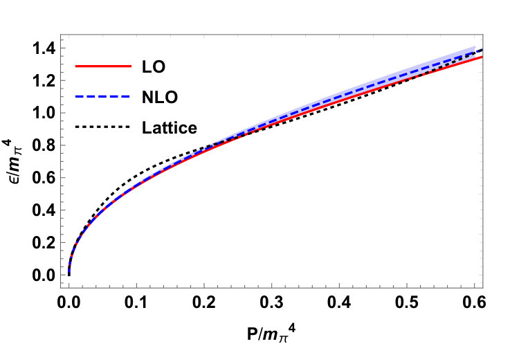 Figure 1
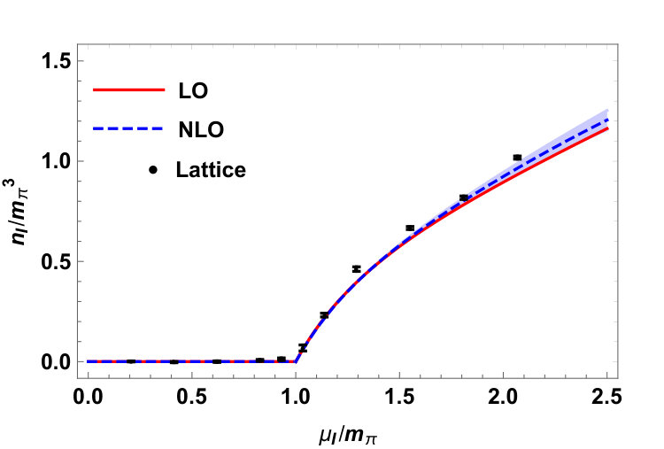 Figure 2
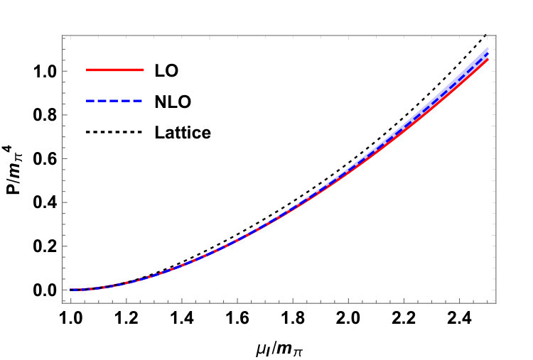 Figure 3
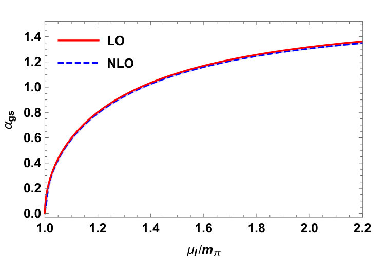 Figure 4
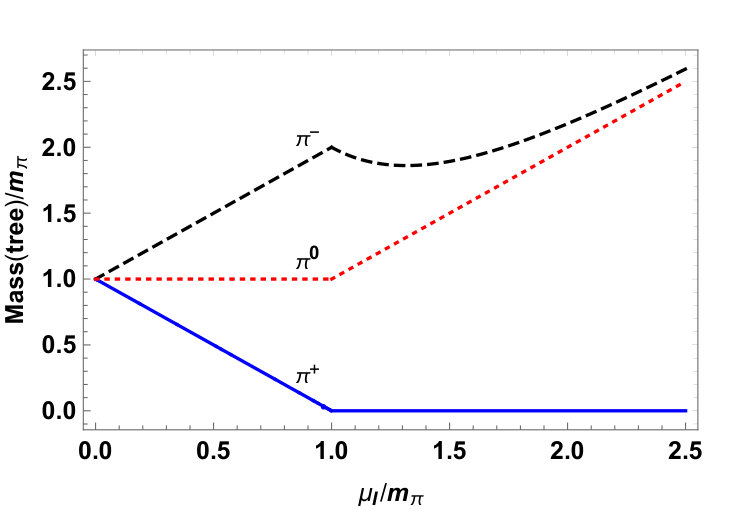 Figure 5
Peer Reviews
No public reviews on file for this paper yet. If you reviewed it on a platform where reviews are public (OpenReview, ICLR, NeurIPS, ICML), you can paste yours below so the community can read it here.
Videos
No videos yet. Explain this paper in a talk, walkthrough, or lecture? Add one.
\thankstext
e1e-mail: [email protected]
\thankstext
e2e-mail: [email protected] \thankstexte3e-mail: [email protected] 11institutetext: St. Olaf College, Physics Department, 1520 St. Olaf Avenue, Northfield, MN 55057, United States
22institutetext: Wellesley College, Department of Physics, 106 Central Street, Wellesley, MA 02481, United States
33institutetext: Department of Physics, Norwegian University of Science and Technology, Høgskoleringen 5, N-7491 Trondheim, Norway
44institutetext: Faculty of Science and Technology, University of Stavanger, N-4036 Stavanger, Norway
Two-flavor chiral perturbation theory at nonzero isospin:
Pion condensation at zero temperature
Prabal Adhikari\thanksrefe1,addr0,addr1,addr2
Jens O. Andersen \thanksrefe2,addr2
Patrick Kneschke\thanksrefe3,addr3
(Received: date / Accepted: date)
Abstract
In this paper, we calculate the equation of state of two-flavor finite isospin chiral perturbation theory at next-to-leading order in the pion-condensed phase at zero temperature. We show that the transition from the vacuum phase to a Bose-condensed phase is of second order. While the tree-level result has been known for some time, surprisingly quantum effects have not yet been incorporated into the equation of state. We find that the corrections to the quantities we compute, namely the isospin density, pressure, and equation of state, increase with increasing isospin chemical potential. We compare our results to recent lattice simulations of 2+1 flavor QCD with physical quark masses. The agreement with the lattice results is generally good and improves somewhat as we go from leading order to next-to-leading order in PT.
††journal: Eur. Phys. J.
1 Introduction
Quantum chromodynamics (QCD), the fundamental theory of strong interactions, has a rich phase structure, particularly at finite baryon densities relevant for a number of physical systems including neutron stars, neutron matter and heavy-ion collisions among others raja ; alford ; fukurev . However, finite baryon densities are not accessible directly through QCD since the physics is non-perturbative and lattice calculations are hindered by the fermion sign problem. Though it is worth noting that some progress has been made in circumventing the sign problem through the fermion bag and Lefschetz thimble approaches bed1 . There is also the additional possibility of solving QCD at finite baryon density with quantum computers since the sign problem is absent in quantum algorithms q1 .
While finite baryon density is inaccessible through lattice QCD, finite isospin systems in real QCD can be studied using lattice-based methods, see Ref. kogut1 ; kogut2 for some early results. The most thorough of these studies were performed only recently gergy1 ; gergy2 ; gergy3 even though finite isospin QCD was first studied over a decade ago using chiral perturbation theory (PT) in a seminal paper by Son and Stephanov son . PT wein ; gasser1 ; gasser2 ; bein is a low-energy effective field theory of QCD that describes the dynamics of the pseudo-Goldstone bosons that are the result of the spontaneous symmetry breaking of global symmetries in the QCD vacuum. Being based only on symmetries and degrees of freedom, the predictions of are model independent.
It is agreed through both lattice QCD and chiral perturbation theory studies that at an isospin chemical potential equal to the physical pion mass there is a second-order phase transition at zero temperature from the vacuum phase to a pion-condensed phase. With increasing chemical potentials there is a crossover transition to a BCS phase with a parity breaking order parameter, or , that has the same quantum numbers as a charged pion condensate. Furthermore, for large temperatures of approximately MeV, the pion condensate is destroyed due to thermal fluctuations. Various aspects of PT at finite isospin density can be found in Refs. son ; kim ; loewe ; fragaiso ; cohen2 ; janssen ; carig0 ; carigchpt ; luca . Finite isospin systems have also been studied in the context of QCD models including the non-renormalizable Nambu-Jona-Lasinio model 2fbuballa ; toublannjl ; bar2f ; he2f ; heman2 ; heman ; ebert1 ; ebert2 ; sun ; lars ; 2fabuki ; heman3 ; he3f ; ricardo ; ruggi , and the renormalizable quark-meson model lorenz ; ueda ; qmstiele ; allofus , with the results found there being largely in agreement with lattice QCD. A very recent review of meson condensation can be found in Ref. mannarev .
In addition to the study of pions at finite isospin chemical potential there has also been recent interest in the study of pions in the presence of external magnetic fields, which are relevant in the context of neutron stars with large fields (magnetars) and possibly in RHIC collisions, which generate magnetic fields due to accelerated charged beams of lead and gold nuclei. In neutron star cores, an isospin asymmetry is present since protons are converted into neutrons and neutrinos through electron capture. However, in the presence of a magnetic field, finite isospin systems are difficult to study due to the fermion sign problem on the lattice QCD that arises as a consequence of flavor asymmetry between up and anti-down quarks for electromagnetic interactions. The complex action problem is tackled by studying finite isospin densities for small magnetic fields, where the sign problem is mild. The lattice observes a diamagnetic phase endromag , while studies in chiral perturbation theory valid for magnetic fields suggests that pions behave as a type-II superconductor prabal .
More recently, due to the accessibility of the equation of state (EoS) of pion degrees of freedom through lattice QCD, there has been a lot of interest in the possibility of pion stars carigchpt ; endro , a type of boson star that does not require the hypothesized axion, which was initially proposed as a solution to the strong CP problem in QCD. Pion stars, on the other hand, only require input from QCD and it is conjectured that pion condensation takes place in a gas of dense neutrinos tomas . Recent work shows that pion stars are typically much larger in size than neutron stars due to a softer equation of state and that the isospin chemical potentials at the center of such stars can be as high as MeV for purely pionic stars and smaller for pion stars electromagnetically neutralized by leptons endro .
The goal of this paper is to revisit the equation of state for finite isospin QCD in the regime of validity of PT, where we expect . The equation of state (at tree level) was originally calculated in Ref. son of QCD. In this paper, we calculate the equation of state within PT and incorporate leading order quantum corrections.
We begin in Sec. 2 with a brief overview of chiral perturbation theory and discuss how to parametrize the fluctuations around the ground state. We derive the Lagrangian that is needed for all next-to-leading order (NLO) calculations within PT at finite isospin chemical potential allowing for a charged pion condensate. In Sec. 3, we use this NLO Lagrangian to calculate the renormalized one-loop free energy at finite . In Sec. 4, we calculate the isospin density, the pressure, and the equation of state in the pion-condensed phase. Our results are compared to those of recent lattice simulations. We summarize our findings in Sec. 5 and present some calculations’ details in Appendices A-E.
2 PT Lagrangian at
In this section, we discuss the symmetries of two-flavor QCD QCD and chiral perturbation theory as a low-energy approximation to it. The two-flavor Lagrangian is
[TABLE]
where is the mass matrix, is the covariant derivative, are the Gell-Mann matrices, and is the field-strength tensor.
For massless quarks, the global symmetries of QCD are , which is reduced to for nonzero quark masses in the isospin limit, i.e. for . If , this is further reduced to . Adding a quark chemical potential for each quark, the symmetry is irrespective of the quark mass. In the pion-condensed phase, the symmetry is broken. In the remainder of the paper, we work in the isospin limit.
We begin with the chiral perturbation theory Lagrangian in the isospin limit at
[TABLE]
where is the (bare) pion decay constant and is the (bare) pion mass. The relation between the physical pion mass and , and between the physical pion decay constant and are briefly discussed in B. The covariant derivatives at finite isospin are defined as follows
[TABLE]
where with denoting the isospin chemical potential and the third Pauli matrix.
It is well known that chiral perturbation theory encodes the interactions among the Goldstone bosons (pions) that arise due to the spontaneous breaking of chiral symmetry by the QCD vacuum, i.e.
[TABLE]
Under chiral rotations, i.e. , the left-handed and right-handed fields transform as
[TABLE]
As such transforms as
[TABLE]
2.1 Ground State
We briefly review the ground state of PT at finite isospin using the Lagrangian. The static Hamiltonian is
[TABLE]
The ansatz for a -dependent rotated ground state can be parametrized by the angle as son
[TABLE]
where . This requirement guarantees that . The static Hamiltonian at then becomes
[TABLE]
The first term in Eq. (LABEL:stath) favors the vacuum direction since the trace of the Pauli matrices is zero, while the second term favors directions in isospin space which anticommute with , i.e. along and . Thus there is competition between these two terms. We also note that the ground-state energy is minimized for . Thus and neutral pions do not condense. By minimizing the above expression with respect to , we get the well-known result that charged pion condensation occurs for with . For , and , i.e. the vacuum solution.
2.2 Parametrizing Fluctuations
Since the goal of this paper is to study the equation of state of the pion condensed phase including quantum corrections, it is natural to expand the PT Lagrangian around the pion condensed ground state. The Goldstone manifold as a consequence of chiral symmetry breaking is . As such, we proceed by first parametrizing the condensed vacuum as follows
[TABLE]
where we, for the purposes of this paper, choose and without any loss of generality. Note that reproduces the normal vacuum with as required. Then the fluctuations (which are axial) around this condensed vacuum are parametrized as
[TABLE]
with
[TABLE]
We emphasize that the fluctuations parameterized by and around the ground state depend on since the broken generators (of QCD) need to be rotated appropriately as the condensed vacuum rotates with the angle kim . 111Consider e.g. a theory with an symmetric Lagrangian with the ground state picking up a vev say in the -direction. If the vev is rotated to the -direction, then the (un)broken generators must be rotated accordingly. We discuss this briefly in C. is an matrix that parameterizes the fluctuations around the ground state:
[TABLE]
With the parameterizations stated above, we get
[TABLE]
As we show later in this paper, this parameterization not only produces the correct linear terms that vanish at , the divergences of one-loop diagrams also cancel using counterterms from the Lagrangian. Furthermore, the parametrization produces a Lagrangian that is canonical in the fluctuations and has the correct limit when , whereby
[TABLE]
as expected.
We would like to emphasize the importance of using and instead of and . If the latter set is used, Eq. (13) is replaced by
[TABLE]
and one finds that the kinetic term of the Lagrangian is not properly normalized. This is in itself not problematic since the canonical normalization can be achieved by a field redefinition. This field redefinition changes the mass and interaction terms of the Lagrangian but only at the minimum of the LO effective potential do the masses coincide with the correct expressions, Eqs. (26)–(29) below. Moreover, if one computes the one-loop effective potential, it turns out that the counterterms cancel the divergences only at the classical minimum. Thus one cannot renormalize the NLO effective potential away from the LO minimum and therefore not find the NLO minimum, which shows that the in Eq. (19) cannot be correct.
2.3 Leading-order Lagrangian
Using the parameterization of Eq. (17) discussed above, we can write down the Lagrangian in terms of the fields , which parametrizes the Goldstone manifold
[TABLE]
where
[TABLE]
The inverse propagator in the basis is
[TABLE]
where is the four-momentum, , and the masses are
[TABLE]
and with representing the inverse propagator for the charged pions. The dispersion relation can be found using the zeros of the inverse propagator . We find that the energies associated with the three pion modes are as follows
[TABLE]
The full propagator can then be written in terms of the dispersion relations as follows
[TABLE]
Expanding the Lagrangian beyond the quadratic terms, we get for terms with three and four fields
[TABLE]
The Lagrangian in the normal phase can be recovered simply by setting . Note in particular that the cubic terms vanish, .
2.4 Next-to-leading order Lagrangian
In order to perform calculations at NLO, we must consider the terms in the Lagrangian that contribute at . In the notation of Ref. gerber , the relevant terms are 222There are additional operators with couplings – and – which are not relevant for the present calculation.
[TABLE]
where – and are bare coupling constants. The bare and renormalized couplings , are related by
[TABLE]
where and are coefficients, and is the renormalization scale in the modified minimal subtraction () scheme (see below). The renormalized s and s are running couplings that satisfy renormalization group equations. Since the bare couplings are independent of the renormalization scale , differentiation of Eqs. (37) – (38) immediately yields
[TABLE]
The low-energy constants and are defined via the solutions to the renormalization group equations (39) as
[TABLE]
and are up to a constant equal to the renormalized couplings and evaluated at the scale gasser1 . The coefficients and are
[TABLE]
Since , Eqs. (38), (39), and (41) obviously do not apply. The coupling is therefore not running, but simply gives a -independent contribution to the effective potential which is the same in both phases. It drops out when we look at the difference in pressure and we ignore it in the remainder of the paper.
In writing the NLO Lagrangian above, we have ignored contributions at finite isospin through the Wess-Zumino-Witten (WZW) Lagrangian, which is of the form
[TABLE]
with the leading contribution at . There is also a separate contribution at zero external field at the same order scherer but neither of these terms through the WZW action contributes to the thermodynamic quantities that we compute at one loop.
Expanding the Lagrangian (36) in the fields, we obtain up to quadratic order
[TABLE]
[TABLE]
[TABLE]
Eqs. (21)–(23) and (34)–(35) from and Eq. (45) from provide us with all the terms we need for the NLO calculation within PT.
3 Next-to-leading order effective potential
The order- contribution to the effective potential is given by minus the static part of the Lagrangian . The one-loop contribution which is of order is given by a Gaussian path integral and is ultraviolet divergent. The ultraviolet divergences must be regularized and we choose dimensional regularization. Dimensional regularization sets power divergences to zero and logarithmic divergences show up as poles in , where is the number of spatial dimensions (see below). The divergences are cancelled by renormalizing the coupling constants appearing in the static part of the Lagrangian , which is also of order-.
3.1 Vacuum phase
The order- contribution to the effective potential is equal to minus the static Lagrangian given in Eq. (21), evaluated at ,
[TABLE]
The dispersion relations for the neutral pion reduces to and for the charged pions . The one-loop contribution to the effective potential is therefore
[TABLE]
The integral is defined as
[TABLE]
where is the renormalization scale in the modified minimal subtraction () scheme and is the number of spatial dimensions. Using Eq. (77), we find
[TABLE]
The static term is given by minus evaluated at ,
[TABLE]
Using Eq. (37) with , the renormalized one-loop effective potential is then given by
[TABLE]
We note that Eq. (53) and therefore the thermodynamic quantities are independent of the isospin chemical potential all the way up to (see Sec. 4), which is the Silver-Blaze property cohen . We therefore refer to this as the vacuum phase. The scale dependence has cancelled in the final result Eq. (53).
3.2 Pion-condensed phase
The order- contribution to the effective potential is equal to minus the static Lagrangian given in Eq. (21),
[TABLE]
Using the dispersion relations for the pions, we can write down the one-loop contribution to the effective potential as follows
[TABLE]
Using Eq. (77), we find
[TABLE]
The calculation of requires isolating the ultraviolet divergences, which can be done by expanding in powers of , which gives
[TABLE]
The ultraviolet behavior of is the same as that of , where E_{i}=\sqrt{p^{2}+m_{i}^{2}+\mbox{1\over 4}m^{4}_{12}} (). Defining \tilde{m}_{1}^{2}=m_{1}^{2}+\mbox{1\over 4}m^{4}_{12}=m^{2}\cos\alpha+\mu_{I}^{2}\sin^{2}\alpha=m_{3}^{2} and \tilde{m}_{2}^{2}=m_{2}^{2}+\mbox{1\over 4}m^{4}_{12}=m^{2}\cos\alpha, the divergent part of the first two terms in Eq. (LABEL:f11) reads
[TABLE]
where we have used Eq. (77). The finite part is defined as
[TABLE]
such that the sum of Eqs. (58) and Eqs. (59) is equal to the first two terms in Eq. (LABEL:f11). The expression for the divergent pieces can be written in terms of using the explicit expressions for , Eqs. (26)–(29). We find
[TABLE]
The static comes from the static part of the Lagrangian, given by minus Eq. (45),
[TABLE]
After renormalization, using Eq. (37) the effective potential has the form
[TABLE]
We note that the all the -dependence cancels in the final result (62). This implies that the thermodynamic functions are independent of the renormalization scale.
4 Thermodynamics
In this section, we investigate the thermodynamics of the pion-condensed phase using the effective potential (62). We will calculate the pressure and the isospin density as a function of the isospin chemical potential , as well as the equation of state, i.e. the energy density as a function of the pressure . In order to evaluate these quantities we need to know the low-energy constants . Evaluated at the scale , they have the following values and uncertainties cola
[TABLE]
The coupling constants and can be measured experimentally via the -wave scattering lengths, while the coupling constant has been estimated using three-flavor QCD gasser1 . Finally, the coupling is related to the scalar radius of the pion and has also been estimated to the value quoted above.
At LO, and and so their uncertainties are the same. Given the values of and , the parameters and at NLO are determined using Eqs. (87) and (88) and the values for the pion mass and the pion decay constant. Since we want to compare our results to lattice data, we choose the same pion mass and pion decay constant gergy11 ,
[TABLE]
The uncertainties in the low-energy constants, , and translate into uncertainties in and . The central values and are obtained by using the central values of , and . The minimum and maximum values of and denoted by and respectively are obtained by combining the maximum and minimum values of the s, , and . The values for the bare pion mass and decay constant are
[TABLE]
We have also considered separately the uncertainties in the LECs and the parameters and . It turns out that the uncertainties are completely dominated by the latter.
The thermodynamic functions are derived from the effective potential (62) at its minimum as a function of so we must first solve
[TABLE]
This can also be used to show that the linear term vanishes on-shell i.e. for the value of that minimizes . We show this explicitly in D.
In Fig. 1, we show the solution to Eq. (69) as function of the isospin chemical potential divided by . The red curve is the order- result, while the blue curve is the order- result. The curves are barely distinguishable.
We first discuss the quasi-particle masses. Restricting ourselves to tree level, the masses are obtained by setting in Eqs. (30)–(31). The normalized masses are shown in Fig. 2 as a function of the normalized isospin chemical potential (both normalized by the pion mass in the vacuum). The mass of the neutral pion is given by the red dotted line, the black curve is the mass of , and the blue line is the mass of .
We see that the pionic excitation is massless for , In the pion-condensed phase, at the minimum of the effective potential. Expanding Eq. (30) around yields
[TABLE]
where we have set which is correct at LO. This shows explicitly that is a massless excitation, which arises due to spontaneous breaking of the symmetry in the pion-condensed phase.
In order to show that there is a second-order transition at a critical chemical potential , we expand the effective potential in powers of up to to obtain an effective Landau-Ginzburg energy functional,
[TABLE]
In E, we carry out the expansion of the effective potential to order using the techniques Ref. split2 . The coefficient can be read off from Eq. (112),
[TABLE]
The critical isospin chemical potential is defined by the vanishing of the coefficient of the term, i.e. . This shows that . In order to obtain this result, we had to take into account the one-loop corrections to the pole mass of the pion and to the pion decay constant expressed in terms of , and the low-energy constants, cf. Eqs. (87)–(88). This result holds to all orders in perturbation theory and is also in agreement with the lattice simulations of gergy1 ; gergy2 ; gergy3 . Moreover, if , the transition is second order. The coefficient can be read off from Eq. (112). Evaluated at , we find
[TABLE]
which is larger than zero. This means that the onset of pion condensation is via a second-order transition exactly at the physical pion mass.
We next turn to the thermodynamic functions. The pressure is given by . Since we are interested in the pressure relative to the vacuum phase we subtract the pressure for , and define
[TABLE]
where the effective potential is evaluated at the minimum. In Fig. 3, we show the pressure normalized to as a function of the isospin chemical potential normalized to . The red curve is the leading-order result, while the blue curve is the next-to-leading order result using the central values of and . The NLO band is obtained by varying the parameters of and as given in Eqs. (66)–(68). We also show the lattice results for the pressure from Ref. endro . The pressure increases steadily with the chemical potential. The NLO pressure increases faster than the LO pressure and is in good agreement with the lattice results.
The isospin density is defined as
[TABLE]
In Fig. 4, we show the isospin density normalized by as a function of the chemical potential normalized by .
The red curves shows the tree-level result and the blue curve shows the one-loop result using the central values of the parameters and . The band is obtained by varying the parameters and as given by Eqs. (66)–(68). We also show the lattice points from Ref. endro . There is no pion condensate in the vacuum up to the critical isospin chemical potential . Hence is independent of , which is an example of the Silver-Blaze property, namely that thermodynamic functions do not depend on all the way up to its critical value cohen . For larger than the critical isospin chemical potential , the density increases steadily. The isospin density as a function of increases as one goes from LO to NLO, and the latter is in better agreement with the lattice results of Ref. endro .
The energy density is defined by
[TABLE]
and can be used to find the EoS. In Fig. 5, we show the normalized equation of state. The LO result is the red curve while the NLO result is the blue curve using the central values of the parameters and . The blue band is obtained by varying the parameters of and as given by Eqs. (66)–(68).
The black dashed line shows the lattice results from Ref. endro . We notice that the NLO equation of state is stiffer than the LO one and that the difference increases steadily with the pressure . Moreover, the NLO EoS is in better agreement with the lattice results for small values of than the LO EoS, while for larger values it is the other way around.
5 Summary
In conclusion, we have derived the PT Lagrangian which is necessary for all NLO calculations at finite isospin. We have applied this Lagrangian calculating the pressure, isospin density, as well as the equation of state. Our predictions are in good agreement with the lattice results of Ref. endro and improves as one goes from LO to NLO. This is the first test of PT in the pion-condensed phase beyond leading order. The Lagrangian we have derived can be used to calculate e.g. the one-loop corrections to the quasiparticle masses in the pion-condensed phase. Here a nontrivial check would be to show that one of the branches is a massless Goldstone boson. The Lagrangian for three-flavor QCD can be derived in the same way and opens up the possibility to study quantum effects in phases that involve pion or kaon condensation. In the case of pion condensation, one can again compare with the lattice results of Ref. endro , as well as between those of the two and three-flavor calculations. This will give us an idea of the effects of the strange quark. Work in this direction is in progress us .
Acknowledgements
The authors would like to thank B. Brandt, G. Endrődi and S. Schmalzbauer for useful discussions as well as for providing the data points of Ref. endro . The authors would also like to thank the Niels Bohr International Academy for hospitality during the later stages of this work. P. A. would like to acknowledge the Faculty Life Committee at St. Olaf College and the Nygaard Study in Norway Endowment for partial travel support.
Appendix A Dimensionally regularized integrals
We need a single integral in dimensions,
[TABLE]
We need several integrals in dimensions. The integrals are defined as in Eq. (50), execpt that the integral is over in Euclidean dimensions.
[TABLE]
The integrals (78) and (79) are standard, while details of the evaluation of (80) can be found in Ref. split2 .
Appendix B Mass renormalization
In order to show the second-order nature of the phase transition to a Bose-condensed phase at , where is the physical mass in the vacuum, we need to express it in terms of the parameters and of the chiral Lagrangian. The relevant terms are found by setting in the and , both evaluated at ,
[TABLE]
The inverse propagator for the pion is
[TABLE]
where the self-energy in the vacuum is
[TABLE]
Here the integral is in Minkowski space. The physical pion mass is defined as the pole of the propagator, or
[TABLE]
Solving this equation self-consistently to NLO and going to Euclidean space yield
[TABLE]
where we have used Eq. (37) with , and Eq. (79). The pion decay constant can be determined in a similar manner, either through the coupling of the axial current to the pion, or by calculating the correlator between two axial currents. The result is gasser1
[TABLE]
Appendix C Rotated generators
Let us consider the rotated parametrization given by
[TABLE]
An infinitesimal fluctuation can be written as
[TABLE]
We can define new rotated generators as
[TABLE]
It is easy to show that the generators satisfy the standard commutation relations of the Pauli matrices. The form of the rotated generators can be understood as follows. The vacuum is rotated in the plane spanned by and , which implies that only the generators in the other directions, i.e. and are rotated. To all orders in , we can write
[TABLE]
Appendix D Equation of motion
The equation of motion for the effective potential in the absence of sources is
[TABLE]
At tree level, the potential is given by minus Eq. (21). Minimizing yields . Comparing Eq. (21) and Eq. (22), we can write
[TABLE]
where is the one-point function at order . We will next show that this relation is satisfied at next-to-leading order, i.e. to order .
The one-loop diagrams contributing to the one-point function arise from the cubic terms in Eq. (34) and shown in Fig. 6. All three pions run in the loop.
In order to work consistently to next-to-leading order, the vertex factors must be evaluated at the classical minimum, or . After Wick rotation, we find
[TABLE]
where () and the one-loop effective potential is given by
[TABLE]
Finally, comparing Eqs. (45) and (46) it is easy to see that
[TABLE]
Adding Eqs. (96), (97), and (99), we find
[TABLE]
at the minimum of . This is the unrenormalized version of the equation of motion. We have checked that the divergences of the one-loop diagram are cancelled by the counterterms up renormalization of the couplings .
Appendix E Expansion in
In this section, we consider the expansion of in powers of . We begin with the tree-level term, which is
[TABLE]
The static term reads
[TABLE]
Now consider the NLO contribution from the charged pions
[TABLE]
which can be rewritten as
[TABLE]
Since , we proceed by expanding in powers of the mass difference, which as we will see is effectively the same as expanding in powers . At , this yields
[TABLE]
The first integral in Eq. (LABEL:splittt) which we denote by can be performed by rewriting the argument of the log in the integrand as
. Then by shifting the integration variable in the first and second pieces respectively, the integral can be written as
[TABLE]
where
[TABLE]
Expanding to yields
[TABLE]
The second integral (labelled as ) reads
[TABLE]
Since the prefactor is and higher, the masses in the integral can be evaluated at since we only care to expand the effective potential up to . Using Eq. (80), we find
[TABLE]
The last contribution is given by Eq. (LABEL:lastcon).
[TABLE]
Adding Eqs. (101), (102), (108), and (111), we can write the one-loop effective potential up to :
[TABLE]
In order to find the critical isospin chemical potential, we set the coefficient of the term to zero and find that at NLO, which can be found using Eqs. (87).–(88). Then evaluating the term at this critical chemical potential gives of Eq. (73), which is positive and therefore at NLO the phase transition remains second order as at tree level.
The reference list from the paper itself. Each links out to its DOI / PubMed record.
- 1(1) K. Rajagopal and F. Wilczek, At the frontier of particle physics, Vol. 3 (World Scientific, Singapore, p 2061) (2001).
- 2(2) M. G. Alford, A. Schmitt, K. Rajagopal, and T. Schäfer, Rev. Mod. Phys. 80 , 1455 (2008).
- 3(3) K. Fukushima and T. Hatsuda, Rept. Prog. Phys. 74 , 014001 (2011).
- 4(4) P. F. Bedaque EPJ Web Conf. 175 , 01020 (2018).
- 5(5) S. P. Jordan, K. S. M. Lee, and J. Preskill, Science 336 , 1130 (2012).
- 6(6) J. B. Kogut and D. K. Sinclair, Phys. Rev. D 66 , 014508 (2002).
- 7(7) J. B. Kogut and D. K. Sinclair, Phys. Rev D 66 034505 (2002).
- 8(8) QCD phase diagram with isospin chemical potential B. B. Brandt and G. Endrődi, Po S LATTICE 2016, 039 (2016).