Efficient estimation of divergence-based sensitivity indices with Gaussian process surrogates
A.W. Eggels, D.T. Crommelin

TL;DR
This paper introduces a novel approach for estimating divergence-based sensitivity indices using Gaussian process surrogates to improve accuracy and efficiency, especially for complex models with limited evaluations.
Contribution
It proposes a new method combining GP surrogates with KDE and introduces direct sensitivity indices for dependent inputs, enhancing sensitivity analysis accuracy.
Findings
GP surrogates improve density estimation accuracy
New divergence-based sensitivity indices for dependent inputs
Enhanced estimation accuracy with fewer model evaluations
Abstract
We consider the estimation of sensitivity indices based on divergence measures such as Hellinger distance. For sensitivity analysis of complex models, these divergence-based indices can be estimated by Monte-Carlo sampling (MCS) in combination with kernel density estimation (KDE). In a direct approach, the complex model must be evaluated at every input point generated by MCS, resulting in samples in the input-output space that can be used for density estimation. However, if the computational cost of the complex model strongly limits the number of model evaluations, this direct method gives large errors. We propose to use Gaussian process (GP) surrogates to increase the number of samples in the combined input-output space. By enlarging this sample set, the KDE becomes more accurate, leading to improved estimates. To compare the GP surrogates, we use a surrogate constructed by samples…
Click any figure to enlarge with its caption.
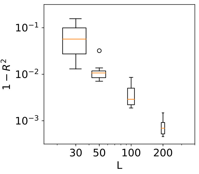 Figure 1
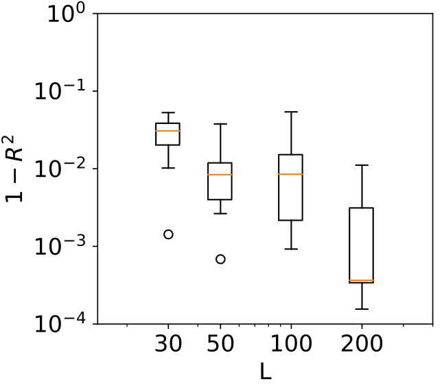 Figure 2
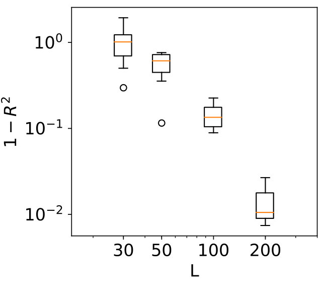 Figure 3
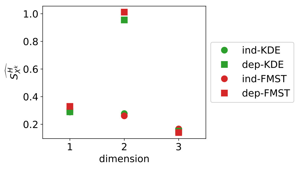 Figure 4
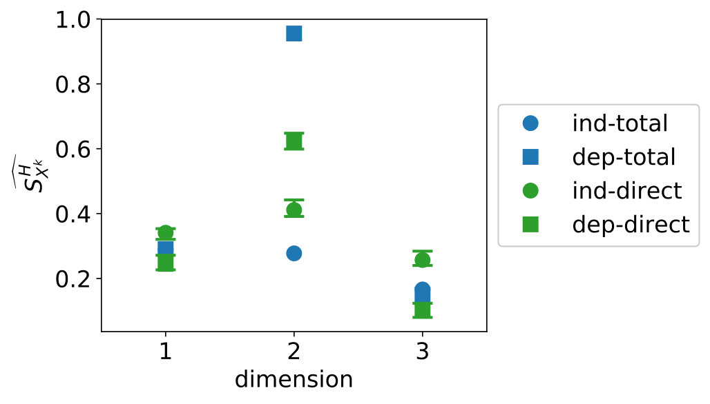 Figure 5
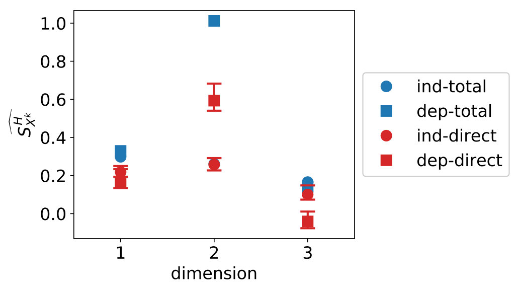 Figure 6
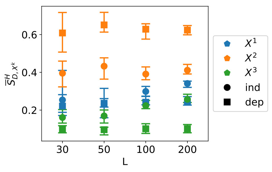 Figure 7
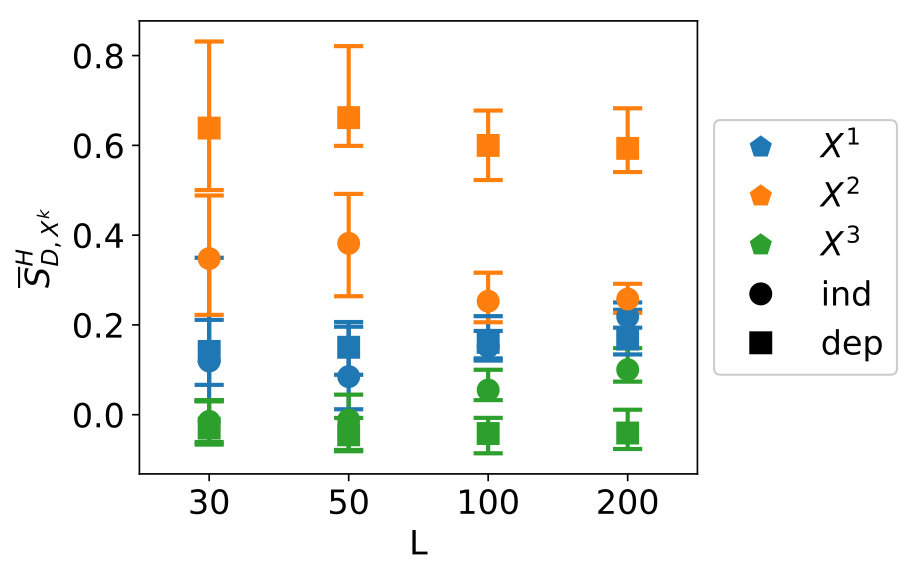 Figure 8
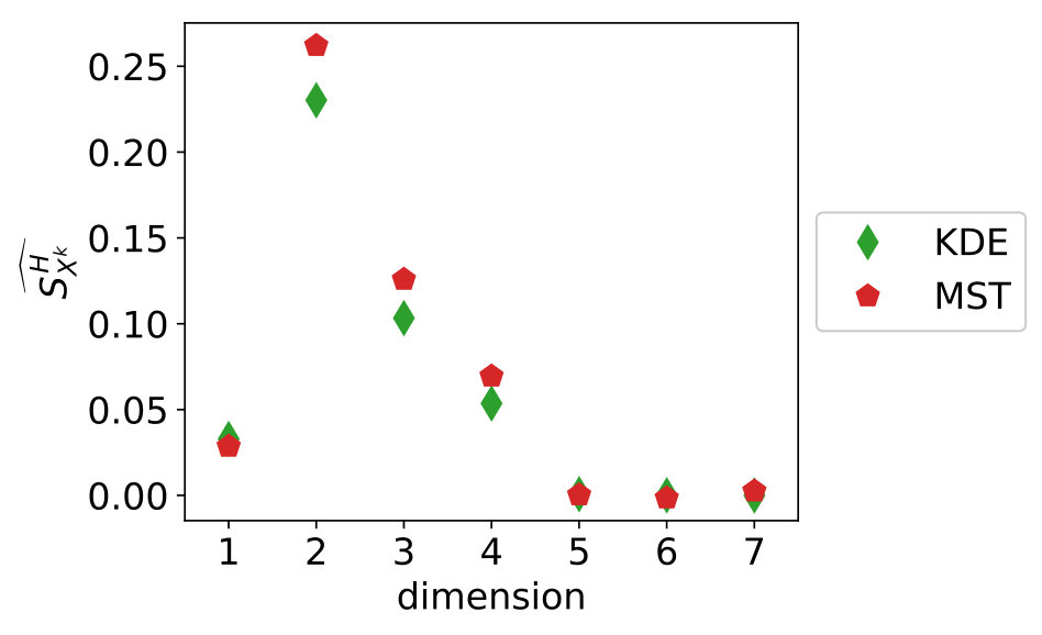 Figure 9
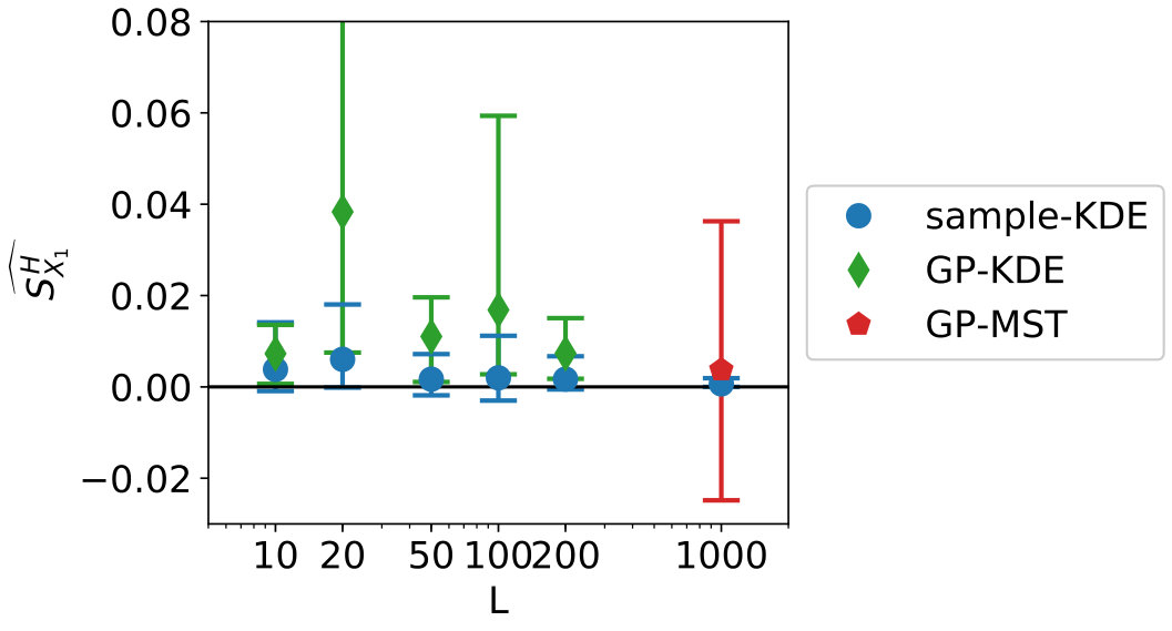 Figure 10
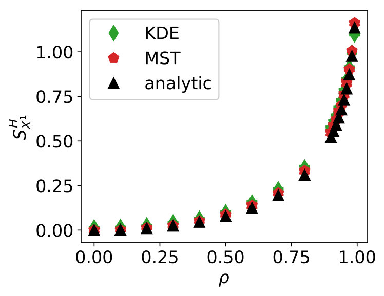 Figure 11
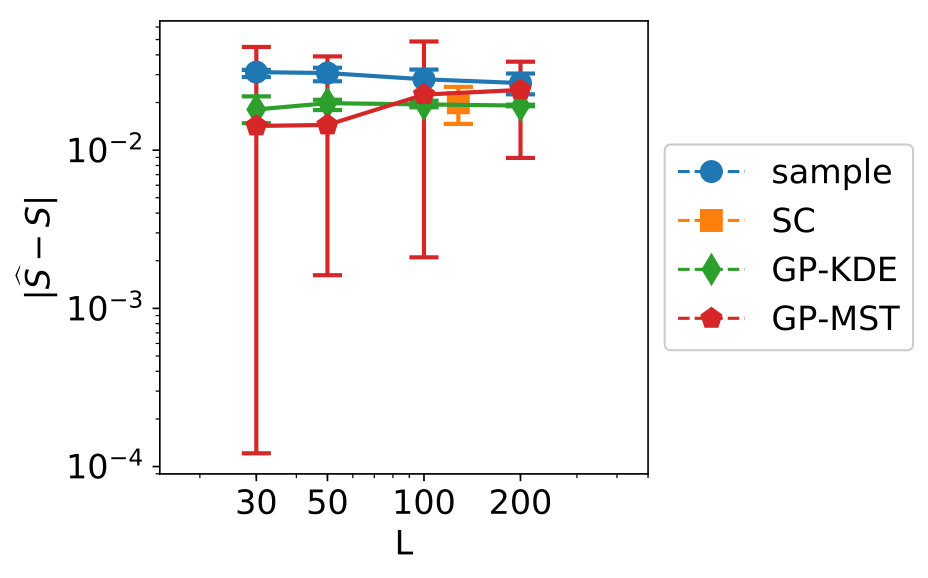 Figure 12
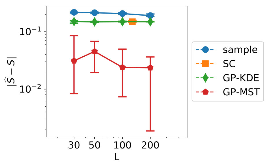 Figure 13
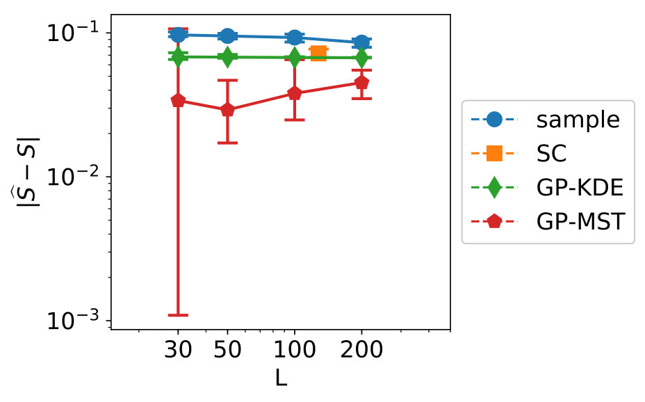 Figure 14
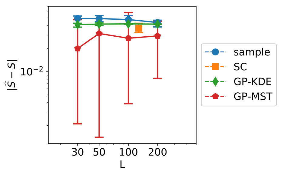 Figure 15
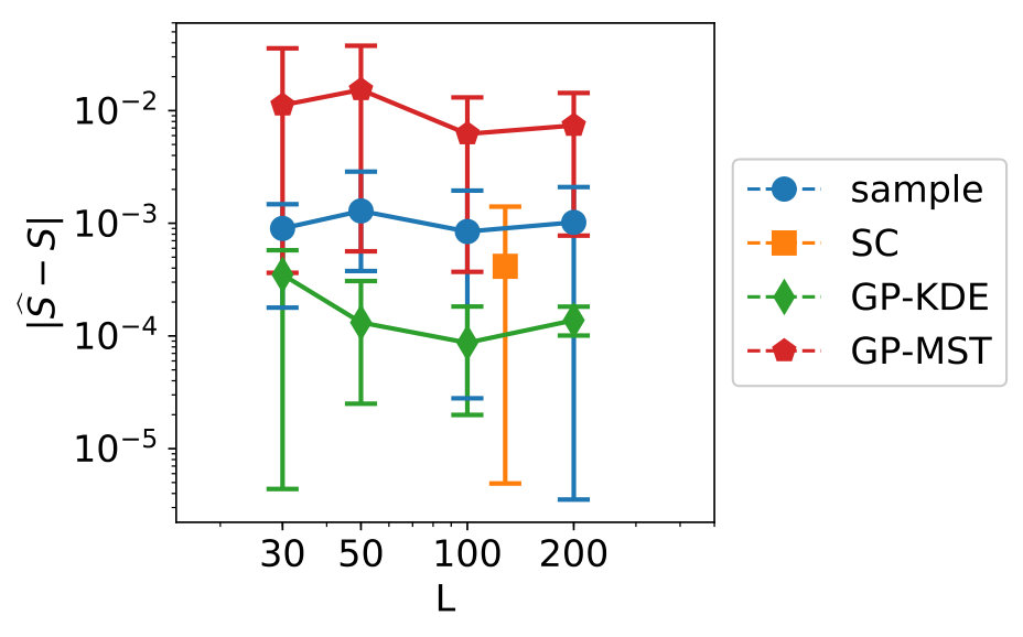 Figure 16
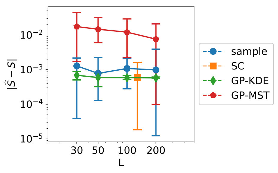 Figure 17
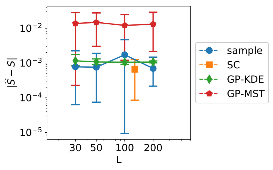 Figure 18
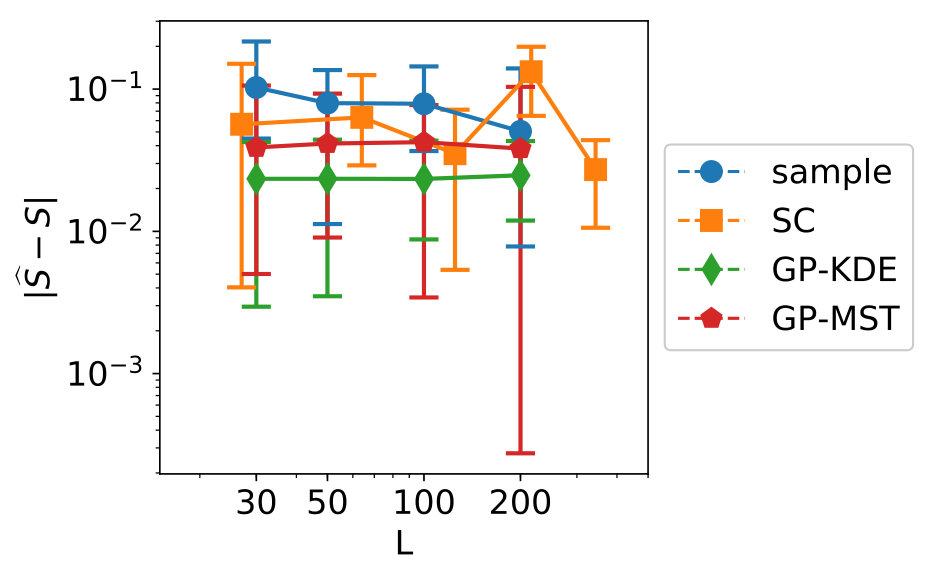 Figure 19
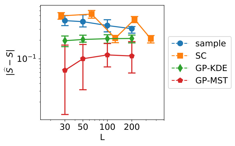 Figure 20
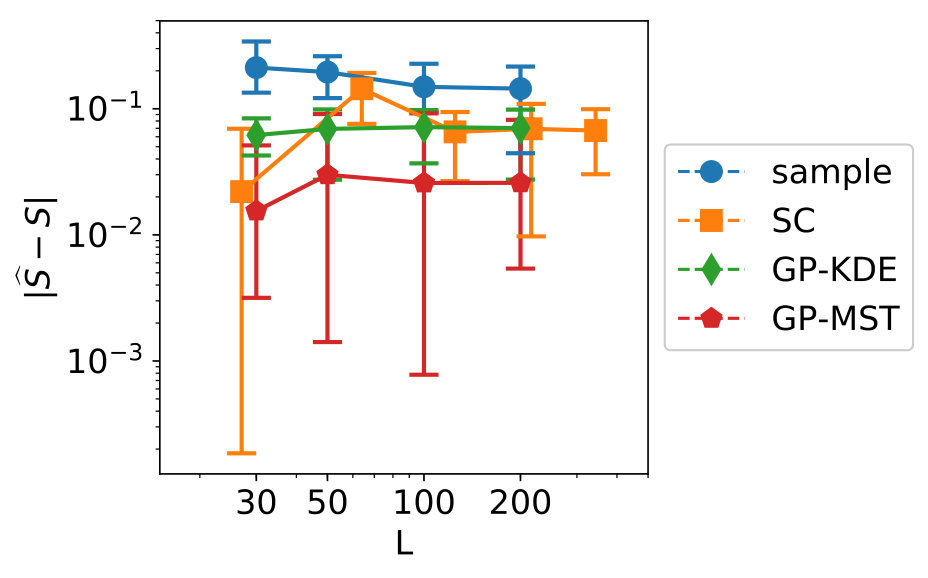 Figure 21
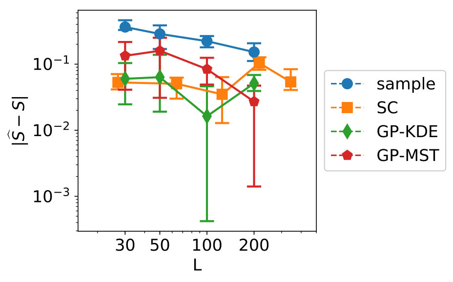 Figure 22
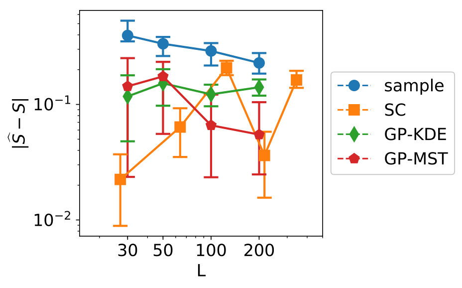 Figure 23
 Figure 24
| Symbol and range | Explanation |
|---|---|
| piston weight (kg) | |
| piston surface area (m2) | |
| initial gas volume (m3) | |
| spring coefficient (N/m) | |
| atmospheric pressure (N/m2) | |
| ambient temperature (K) | |
| filling gas temperature (K) |
Peer Reviews
No public reviews on file for this paper yet. If you reviewed it on a platform where reviews are public (OpenReview, ICLR, NeurIPS, ICML), you can paste yours below so the community can read it here.
Videos
No videos yet. Explain this paper in a talk, walkthrough, or lecture? Add one.
Taxonomy
TopicsProbabilistic and Robust Engineering Design · Advanced Multi-Objective Optimization Algorithms · Optimal Experimental Design Methods
Efficient estimation of divergence-based sensitivity indices with Gaussian process surrogates
A.W. Eggels, D.T. Crommelin
Abstract
We consider the estimation of sensitivity indices based on divergence measures such as Hellinger distance. For sensitivity analysis of complex models, these divergence-based indices can be estimated by Monte-Carlo sampling (MCS) in combination with kernel density estimation (KDE). In a direct approach, the complex model must be evaluated at every input point generated by MCS, resulting in samples in the input-output space that can be used for density estimation. However, if the computational cost of the complex model strongly limits the number of model evaluations, this direct method gives large errors. We propose to use Gaussian process (GP) surrogates to increase the number of samples in the combined input-output space. By enlarging this sample set, the KDE becomes more accurate, leading to improved estimates. To compare the GP surrogates, we use a surrogate constructed by samples obtained with stochastic collocation, combined with Lagrange interpolation. Furthermore, we propose a new estimation method for these sensitivity indices based on minimum spanning trees. Finally, we also propose a new type of sensitivity indices based on divergence measures, namely direct sensitivity indices. These are useful when the input data is dependent.
1 Introduction
Sensitivity analysis is an essential part of uncertainty quantification and a very active research field [1, 2, 3]. Several types of sensitivity indices have been formulated, such as variance-based (including Sobol’s indices [4]), density-based [5], derivative-based [6] or divergence-based. Broadly speaking, divergence-based sensitivity indices quantify the difference between the joint probability distribution (or density) of model input and output on the one hand, and the product of their marginal distributions on the other hand. A variety of divergence-based indices can be brought in a common framework built on the notion of -divergence [7], as was shown by Da Veiga [8]. The -divergence is a generalization of several well-known divergences such as the Kullback-Leibler divergence [9] and the Hellinger distance [10].
In most cases, these sensitivity indices cannot be computed analytically because the distribution of the model output given the input is not known exactly. As an alternative, one can resort to Monte Carlo (MC) sampling combined with kernel density estimation: the input distribution is sampled using MC, the model is evaluated on all sampled input points, and from resulting input-output points the joint and marginal probability densities of input and output are estimated. However, when the number of available output points is low, for example because of high computational cost of the model, the estimated densities will generally be inaccurate, resulting in large errors in the estimated sensitivity indices.
In this study we first propose to increase the number of output samples by using a Gaussian process (GP) surrogate. The GP is constructed on the input-output points that are obtained with the (expensive) model. The main idea is that the additional output samples improve the kernel density estimates even though they introduce a bias due to the difference between the true model and its GP approximation. Our approach is based on both the development of divergence-based indices and the use of Gaussian processes in sensitivity analysis. Therefore, we briefly summarize some of the advancements in these areas. Auder & Iooss [11] presented two sensitivity analysis methods based on Shannon and Kullback-Leiber entropy, respectively, building on work in [12] and [13]. Da Veiga [8] introduced sensitivity indices based on the -divergence. Recently, KDE also appears in estimators of mutual information measures in [14], where -divergences are computed between the joint distribution of two random variables and the product of their marginal distributions. In [15], -divergence measures are computed by a -nearest neighbor graph.
The use of GPs is discussed in Marrel et al. [16], together with the analytical expressions for Sobol indices that arise from them. To compute the indices, two approaches are considered: one in which the predictor of the GP is used and one in which the full GP is used. The latter approach is found to be superior in convergence and robustness. Furthermore, the modeling error of the GP is integrated through confidence intervals; it is reported that the bias due to the use of the GP is negligible [16]. In a related study, Svenson et al. [17] estimate Sobol indices with GPs, using specific compactly supported kernel functions. Furthermore, combining GPs with derivative-based indices has been investigated by [6] and [18]. In [19], predictions from a GP are used to rank the input variables based on their predictive relevance. Two methods for this are presented in [19], one based on Kullback-Leibler divergence and one based on the variance of the posterior mean.
Despite the developments sketched above, approaches that combine GP surrogate modeling and divergence-based sensitivity analysis have not been explored much yet, although [20] already applied this approach. The methodology proposed in this paper combines these two elements.
We note that for the approach proposed here it is not needed to assume that the inputs are mutually independent, nor does dependency of inputs make it more complicated. We present test cases with independent inputs as well as cases with dependent inputs. For the former, we compare with results obtained with stochastic collocation [21, 22]. In this method, an appropriate set of points, called collocation points, is obtained. These are usually chosen as the zeros of the orthogonal polynomials with respect to the marginal input probability distributions. Then, Lagrange interpolation is used to approximate the output function. For dependent inputs, this method might not be ideal, as [23] already showed.
Second, we propose a new estimation method for the divergence-based sensitivity indices as introduced before. Because the KDE method depends on the choice of both kernel and kernel bandwidth, we propose to use an estimator without parameters which is numerically fast as well. This estimator is based on the approximation of one of the integrals appearing in the sensitivity index by computing a minimum spanning tree [24].
As a third contribution, we propose a new set of sensitivity indices to complement the ones introduced before. This new set computes the direct sensitivity indices, which measure the sensitivity of the output with respect to one input variable only. This is beneficial for cases when the input variables are dependent, because these indices remove indirect effects caused by dependent input variables. To illustrate this, consider an example where follows a bivariate normal distribution with means [math], variances and covariance , while . Then the direct effect of on the output is zero, while the original sensitivity index would be positive due to the dependence between and .
Section 2 describes the sensitivity indices central to this paper, their estimation method and the complications therein. It also contains our proposed method to enlarge the set of input and output data and the new estimation method. Section 3 applies these estimators to several test cases. Section 5 concludes.
2 Divergence-based sensitivity indices and their estimation
We start by introducing the sensitivity indices derived from the -divergences in Section 2.1. Section 2.2 discusses the complications in estimating them. Gaussian processes and the two estimators are given in Section 2.3.
2.1 Sensitivity indices from the -divergence
We consider the situation where a model takes a vector of inputs and returns a (scalar) output . The input vector is random, and as a result the output is a random variable as well. Da Veiga [8] proposed to perform global sensitivity analysis with dependence measures, especially -divergences (see also [25]). In this way, the impact of the th input variable on the output is given by
[TABLE]
where denotes a dissimilarity measure. The unnormalized first-order Sobol indices can also be written in this framework, namely with
[TABLE]
We will use the Csiszár -divergence [7], which is given by
[TABLE]
with a convex function with , and denotes a probability distribution function. Some well-known choices for are (Kullback-Leibler divergence) and (Hellinger distance). Combining (1) and (2) with basic probability theory gives us
[TABLE]
These sensitivity indices are equal to zero for and independent and positive otherwise. Furthermore, they are invariant with respect to smooth and uniquely invertible transformation of and [26], in contrast to Sobol indices which are only invariant with respect to linear transformations. Moreover, it is easy to generalize (3) to multidimensional .
2.2 Difficulties for estimation
The main problem for computing is that the probability densities in (3) are not known. In order to estimate it is necessary to estimate and , and, depending on the type of input, as well. In [8] it is indicated that if samples are available, only the ratio needs to be estimated.
The estimates of the densities can be obtained with kernel-density estimation (also in [8, 25]). To do so, one chooses a suitable kernel and a suitable value for the kernel bandwidth . When the density of the input is known, this information can be used to determine , otherwise, guidelines are available [27].
Clearly, the estimate of the density will not be perfect, leading to an error in the estimation of . This is strongly related to the number of samples available for density estimation. If high computational cost of the model limits this number, the estimation of can be improved by using a surrogate of the model to generate more samples. One possible way to do so is to use stochastic collocation (SC) [21, 22]. Herein, one chooses the samples as the collocation points, which are obtained as the zeros of the orthogonal polynomials with respect to the marginal input distributions. Then, at these collocation points, the corresponding output samples are obtained. Finally, an emulator is constructed by Lagrange interpolation on these samples.
As an alternative, we propose to use Gaussian processes [28] as a surrogate model to obtain the larger sample , in which indicates the surrogate model output for the extra input samples . For each data point in , this is a normal distribution in itself, and for each point in it is a degenerated normal distribution (i.e., it has zero variance). An additional advantage may be the availability of confidence intervals for at almost no extra computational cost. Unfortunately, these confidence intervals do not include the bias from approximating the output by a Gaussian process.
2.3 Estimation using Gaussian processes
We assume the input samples are already available, otherwise one can use Monte Carlo sampling (or Latin hypercube sampling in the case of independent uniform data) to select samples from the data . Although it may be tempting to use other sample selection methods, it is not guaranteed that they represent the distribution just as naive sampling would. Then, the corresponding output can be obtained as with the process to generate output, which is either a function or a computational model. Then, one needs to fit a Gaussian process to , thereby choosing an appropriate kernel. This Gaussian process is now used to obtain output for other input samples . This leads to the augmented dataset of size with (partial) surrogate output . Note that does not consist of single values, but rather of multivariate normal distributions.
2.3.1 Kernel density estimation
We now explain how to compute the KDE on and how it is used to approximate (3). Because is computed per input variable , it is here enough to consider one-dimensional kernel densities.
For each input variable and output variable , the estimators for the kernel density are given by [25]:
[TABLE]
with the th sample of the input data and the size of the data. Note the input data has to represent the distribution of . An extension to a higher-dimensional is easy to obtain. For our purpose, we either have and , or we have and . We choose the Gaussian kernel and according to Scott’s rule [29, p. 152], which is optimized with respect to the normal distribution. Then, the estimator for as given by [25] is obtained:
[TABLE]
We note this choice of may not be optimal. We have adapted the bandwidth previously to the ranges of and , but the results of this are worse than with a single bandwidth. Also, kernel density estimation may not be the best choice when the domain of a variable or is bounded and this variable has nonzero density at the boundaries.
Until so far, we ignored the fact is a multivariate normal random variable instead of a single value when . Therefore, there are two options to obtain values for . The first option is to use the prediction mean and get the resulting output samples
[TABLE]
to be used in (4). The other is to sample from this normal distribution times. In that case, one gets the output sets
[TABLE]
in which denotes “sampled from the distribution”, and thereby estimates of . Note that this also implies the kernel density estimates have to be computed times. Because the computation of the kernel density estimate is expensive, we choose not to include this option. We will indicate the estimator by in the results, where the value of is clear from the context.
2.3.2 Minimum spanning trees
Before we can explain how to use the minimum spanning trees, we first need to introduce the concept of Rényi entropy. This is a generalization of the continuous Shannon entropy (see e.g. [30]) and is given by
[TABLE]
for . In the limit of , the Rényi entropy converges to the continuous Shannon entropy. Hero & Michel [31, 24, 32] proposed a direct way to estimate the Rényi entropy for given a dataset consisting of samples of the probability distribution of dimension . Their estimator is
[TABLE]
in which can be derived from the relation . The functional is given by
[TABLE]
in which denotes the set of spanning trees on and denotes an edge therein. The parameter can be computed from the desired value of and will be within the interval . The constant is defined by
[TABLE]
for a sample of size of the uniform distribution in dimensions. However, we will estimate it for samples only by computing it for several repetitions of the sample .
The estimator (7) is asymptotically unbiased and strongly consistent for [33]. We focus on the case and wherein denotes the Euclidean distance, hence . To see why we choose , we give the following derivation. First, we need to introduce the Rényi divergence by
[TABLE]
for the probability distribution functions and . We choose and , where is the joint probability distribution function of and and and denote the marginal probability distribution functions. Then, their Rényi divergence is given by
[TABLE]
We also have
[TABLE]
with the (well-defined) probability distribution function given by
[TABLE]
We also see that , with denoting the sensitivity index derived from the Hellinger distance, is given through (3) by
[TABLE]
which can be simplified to
[TABLE]
We now see the agreement between (10) and (12). In case the domain of and is extended to by zero density outside of the domain, it is possible to write
[TABLE]
with
[TABLE]
hence
[TABLE]
We can compute via (Equation 11). Therefore, we need to estimate (8) and (9). Because can be estimated as
[TABLE]
we estimate the sensitivity indices by
[TABLE]
3 Results
We test the estimators in several ways. The first test case is with regard to random input/output data and is described in Section 3.1. In this case, the estimates should be near zero. The second test case, in Section 3.2, is based on comparing analytic to numerical values of the sensitivity indices. In the third test case, the Ishigami function is used and tests are performed for both independent and dependent input data, of which the results can be found in Section 3.3. The last test case is higher-dimensional and considers the Piston function (Section 3.4). In these tests, we only use the Hellinger distance. All experiments have been performed times. The error bars in the upcoming figures indicate the minimum and maximum value found. The results are summarized in Section 3.5.
3.1 Random data
First, we check the behavior for random output, in which case the sensitivity indices should be zero. Both the input and output data are one-dimensional, uniformly distributed on and have size , while is varied from to based on [34]. The results are in Figure 1.
On the right, we show the sensitivity index as computed on the complete, i.e., , data by KDE and MST (blue circle and red pentagon). Herein, no Gaussian process is used. As expected, their mean is around zero. The spread for the KDE method is smaller than for the MST method. The estimates for based on samples (blue circles) are also around zero, although their spread is larger than for . Note that due to the numerical implementation, the sensitivity indices can become negative.
We continue with the estimates based on Gaussian processes. Herein, the situation is a little different because the Gaussian process fits a function through the data while there is no functional relation between input and output. Hence, the sensitivity indices will most likely not be equal to zero. When fitting the Gaussian process, two cases appear, which have the same effect. The length scale and the process variance are either both small or both large. As a result, the predictions of the Gaussian process will be inaccurate. This can be seen in the figure for the KDE results (green diamonds) by their mean being away from zero and the large spread of their estimates (the outlier has a value of approximately ). However, due to the nature of this method, high values of are measured because the predicted output values are the values of the prediction mean function, which is a continuous function. Hence, these predictions are located on a curve. Therefore, the values of for the MST-based estimator are too large to be visible in this plot for the chosen values of , except for , where no emulated output is used. The reference result where we computed the FMST-based sensitivity index on the full data without emulator gave a reasonable result (red pentagon).
Similar results appear for estimates based on emulation by stochastic collocation (SC), where we used collocation samples based on the uniform distribution. A function is fit through the data while no functional relation between input and output exists. Therefore, high values of are measured, which are not shown in the plot.
We summarize these results as follows: when an emulator (either Gaussian process or SC) is used to augment the data for sensitivity analysis, positive values of are found because the emulator is designed to fit a functional relation between input and output. The “sample” method does not suffer from this problem. However, this is a very specific test case in which sample-based estimators are preferred over ones which use an augmented dataset.
3.2 Analytic test case
We consider a small test case in which we can compute the sensitivity index analytically. The idea behind this is to compare the KDE and the MST method in case no emulator is used. We have
[TABLE]
We took and repeated the experiment times. The results are in Figure 2.
Except for , the MST method outperforms the KDE method. Furthermore, the MST method is i) not dependent on parameter choices such as kernel and kernel bandwidth and ii) faster to compute. One also needs to take into account that the rule of thumb to choose the kernel bandwidth we used here is based on the assumption that the data comes from a normal distribution and, therefore, this kernel bandwidth is optimal in this test case. When the underlying distribution is not normal, this heuristic may not be optimal.
3.3 Ishigami function
We now continue to a non-trivial synthetic test case, of which the test function is from Ishigami & Homma [35]. This output function is defined by
[TABLE]
on the domain (dimension ). We will use the well-known choice , in accordance with [36].
Two types of input data are constructed for this test case. One is uniformly distributed and consists of samples on the domain of the output function. The other is the empirical copula of a multivariate normal distribution on the same domain, which is given by
[TABLE]
such that
[TABLE]
with the cumulative distribution function of the marginal distributions (which is distributed as ).
For reference, we compute both the KDE-based and MST-based estimate on a larger dataset (with ) for comparison. Scott’s rule [27] is used for the kernel bandwidth.
In the numerical experiments, we first compute, depending on the dataset, a Latin hypercube sample (LHS) or Monte Carlo sample (MCS) of size and combine it with KDE. For this data, we computed (4). Then, we fit a Gaussian process with Gaussian kernel to these samples, where the length scales have been estimated by maximum likelihood estimation. Now, we can proceed with KDE on , in which we include the choice (Equation 5). We obtain one estimate for for each repetition of the experiment and thereby one value of which is used as measure of convergence. In a similar way, we can proceed with the MST method on with . Finally, the SC method, based on the uniform distribution and combined with KDE, is used for comparison. Note we showed earlier that KDE has a larger bias than MST, but we look mainly at the convergence here.
The computed reference values of the sensitivity indices are shown in Figure 3.
The values for independent and dependent data are close to each other for variables and , while they are far apart for variable , which is due to the dependency.
We will first show the results for the independent data, followed by the results for the dependent data. We start with determining the goodness-of-fit of the Gaussian process by performing -fold cross-validation (CV) with and compute the coefficient of determination
[TABLE]
where are the CV predictions for and .
The values for for independent data are given in Figure 4 and we see its values are near zero for higher values of . For and , this fraction can become larger than . In this case, the fit is worse than a constant function. Note that here, the Gaussian process is not fit well, while this is the case for the higher values of .
Figure 5 shows the convergence of the estimates, where “sample” indicates the KDE is based on only samples, “SC” indicates stochastic collocation is used (combined with KDE), “GP-KDE” is based on (5) and “GP-MST” is based on (13). From left to right, variables 1 to 3 are shown. This will also be the case for all similar figures in this section.
In this figure, we see several trends. First of all, the samples perform worse than the methods which use augmentation of the dataset. Second, we see the results for SC are not robust and their errors do not decrease in general for increasing . Third, we see that GP-MST shows in general decreasing errors for increasing .
The results for dependent data are shown in Figures 6 and 7. Note that LHS is not an appropriate sampling method because the data is dependent, therefore, Monte Carlo sampling is used instead. Furthermore, SC is here also not completely suitable because the input distribution is dependent. The results are similar to previous experiments, although the cross-validation results imply the Gaussian process for this data has been fit better. Another observation is that GP-MST outperforms the other methods for variables 2 and 3, while it is not really worse than GP-KDE for variable 1. Overall, the Gaussian process-based methods outperform the other methods.
3.4 Piston function
We also tested a higher-dimensional test case with independent uniformly distributed input variables. In this case, the output function is defined by the Piston function from [37]. The output here is the cycle time of a piston, as given by
[TABLE]
of which the input ranges are given in Table 1.
For numerical reasons, the data of size is generated and processed on the unit hypercube: it is only transformed to the input ranges to obtain the output values. The sensitivity indices as computed on a larger dataset of size are given in Figure 8. The values for KDE and MST differ, although Section 3.2 indicates the MST results are more accurate.
The cross-validation results are in Figure 9. These last results show the Gaussian process has been fit well for and therefore we can continue with the remaining results.
The results for the convergence are in Figure 10. From left to right, top to bottom, variables 1 to 7 are shown.
We see clear differences between variables 1-4 on one hand and variables 5-7 on the other hand. This is due to variables 5-7 for which is near zero. As indicated in Section 3.1, methods which make use of a fit perform badly in this case. For variables 1-4, GP-MST clearly outperforms the others. The SC method has only been performed with collocation points for each dimension, which led to . Increasing to would give us collocation points, which is higher than the number data points in the used dataset.
3.5 Recommendation
The Gaussian process-based methods in general outperform the sample-based method and stochastic collocation, except when the value of the sensitivity index is (near-)zero. However, usually one is interested in ordering the input variables based on the sensitivity indices rather than obtaining their values very precisely. Input variables with values of the sensitivity index near zero are usually considered unimportant and in that case, it is also not very important to estimate the value of zero very precisely. We therefore advise to use the GP-MST method, wherein the available samples are augmented to by a Gaussian process, on which the sensitivity index (3) is computed for the Hellinger distance by the minimum spanning tree method.
4 Direct sensitivity indices
We note that the sensitivity indices as described by [8] are total sensitivity indices, which include both direct and indirect effects. Direct effects measure the effect of one input variable only, while indirect effects contain the effect of the other variables due to possible dependencies in the input variables. The indirect effect is the difference between the total and the direct effect. To illustrate this, consider an example where follows a bivariate normal distribution with means [math], variances and covariance (so that and are dependent), while . Then the direct effect of is zero, while its total effect is positive (because and are dependent through ). Hence, the indirect effect of is positive as well. Our goal is now to find a measure for the direct effects, i.e., without the effects of the mutual input dependencies.
Although useful, total sensitivity indices do not tell the complete story. While an input variable may be completely irrelevant for the value of the output, it may have a positive sensitivity index due to a dependency with a relevant input. The relevant input variable would then be called a confounder. An example of this is wave height for a computational model of offshore wind energy: although the waves have nothing to do with the power output, they are linked to each other via the wind speed with which they have a dependency. To get rid of this effect, we need to construct indices which measure the effect of only one input variable, without effects due to dependencies in the input. It is in this case necessary to remove the dependencies from the input.
For variance-based sensitivity indices, a distinction is made between first-order, higher-order and total sensitivity indices [38]. In first-order indices, one only measures the effect of varying one variable alone, where in higher-order indices multiple variables are varied at the same time. Because the number of second-order sensitivity indices grows as with the number of input variables, and the total number of sensitivity indices is , usually not all of them are computed. Instead, one computes the first-order and total sensitivity indices.
In a similar fashion to first-order indices, we define direct sensitivity indices, which measure the effect of varying one variable only. The direct indices then measure the direct effects, while the total indices measure the combination of direct and indirect effects, which also includes effects due to dependencies in the input.
4.1 Theory
The starting point of these new indices is the same divergence-based index as before, namely (12). We repeat (12) here for convenience,
[TABLE]
Now, note that
[TABLE]
with being the model used to obtain the output , hence, both and depend in theory on all input variables . Hence, if we remove the dependencies between the input variables, then these probability distributions change as well. This removal is done by applying a permutation operator , which is defined on a dataset in such a way that
[TABLE]
with
[TABLE]
Hence, this operator keeps the marginal distributions the same, but it removes all dependencies ( here denotes statistical independence). The implementation of this operator is detailed at the end of this section.
Now, we create a permuted version of our dataset , being . For this dataset, we can define the direct sensitivity index by
[TABLE]
The output can be replaced by
[TABLE]
in which denotes the Gaussian process constructed earlier. This leads to the estimator
[TABLE]
The problem now is how to define . A naive implementation could be one in which for each variable, a random permutation of the values is performed. This is fast, but does not guarantee independence of the input variables after transformation. Also, the indexing of the permutations leads to a Latin hypercube design (LHD): each value from to (for data points in the dataset) is used only once. However, this does not guarantee all dependencies are removed. In Latin hypercube sampling (LHS), a comparable problem exists as equally probable subspaces can end up with a different number of sampling points. This is solved by orthogonal sampling [39] or by using a maximin criterion [40].
Inspired by this, we would like to generate an LHD of size in dimensions with the maximin criterion which puts the samples at the middle of each interval. This LHD is easily transformed to an indexing, which can be applied to the original data to obtain . However, obtaining such an LHD is computationally very expensive because it contains an optimization step and is therefore not feasible for the problem sizes we are looking at.
An alternative to Latin hypercube sampling is quasi-Monte Carlo sampling, which generates data points from low-discrepancy sequences such as Halton’s [41, Chapter 3] and Sobol’s [42]. In this way, we achieve the goal that the proportion of data points in a sequence falling into a subspace is nearly proportional to the probability measure of this subspace (the difference between them is the discrepancy). Hence, we achieve an approximately uniform distribution of data points over the unit hypercube, which means the dimensions are independent of each other. Furthermore, all values generated for a variable are unique, which means they can easily be transformed to the discrete hypercube . The transformed values can be used as an indexing for to obtain . Because the data points generated by the sequence are uniform over the unit hypercube, they lead to an independent dataset when their transformed values are used as indexing. We use the Sobol sequences as described by [42].
4.2 Ishigami
We compute these direct sensitivity indices for the Ishigami test case of Section 3.3. We split the results out to the KDE and the MST estimates. For each of them, we show the estimates of both the independent and dependent direct sensitivity indices and the spread therein for increasing . We also compare them to the values of the total indices.
We start with the KDE estimates in Figure 11. On the left, we see that the estimates are relatively stable for increasing and the spread of the estimates decreases. On the right, we compare the estimates for for the direct indices to the estimates with for the total indices. We do not compute a reference value for the direct indices because of computational cost. For the dependent data, the indices work as expected: the total indices are larger than the direct sensitivity indices. For the independent data, this is not the case, as for variable 2 and 3 the direct sensitivity index is larger than the total sensitivity index. It is not immediately clear to us why this is the case, because for independent data, the total and direct sensitivity indices should give the same results.
Figure 12 shows on the left similar results for the stability and spread in the estimates as before with KDE. On the right, we see the total sensitivity indices are larger or equal than their direct sensitivity indices counterparts. For the independent data, the differences between the the direct and total sensitivity indices are small for variable 1 and 3 and nearly invisible for variable 2. Theoretically, this difference should be (numerically) zero. For the dependent data, we see the difference between direct and total sensitivity index is largest for variable 2, while variables 1 and 3 show a small difference. This is due to variable 2 being stronger dependent with the other two variables.
5 Conclusion
We proposed to use Gaussian processes in order to improve the estimates of divergence-based sensitivity indices. This is advantageous in cases where the number of available input-output samples is small, for example if the computational cost of each model evaluation needed to compute the output is high.
We compared the use of Gaussian processes to the well-established method of stochastic collocation combined with Lagrange interpolation. This method has several disadvantages in practice and is outperformed by the Gaussian process-based methods in our experiments. The use of Gaussian processes also allowed us to propose (i) a new estimation method and (ii) a new type of sensitivity indices. This new estimation method for divergence-based sensitivity indices is based on minimum spanning trees and can be used in case the divergence used is the Hellinger distance. This estimation method has been used before to compute entropies and is numerically fast. The new type of sensitivity index, named direct sensitivity index, is especially useful when the input data is dependent.
Acknowledgments
This research is part of the EUROS programme, which is supported by NWO domain Applied and Engineering Sciences under grant number 14185 and partly funded by the Ministry of Economic Affairs.
The reference list from the paper itself. Each links out to its DOI / PubMed record.
- 1[1] A. Saltelli, Global sensitivity analysis: an introduction, in: Proc. 4th International Conference on Sensitivity Analysis of Model Output (SAMO’04), 2004, pp. 27–43.
- 2[2] J. E. Oakley, A. O’Hagan, Probabilistic sensitivity analysis of complex models: a Bayesian approach, Journal of the Royal Statistical Society: Series B (Statistical Methodology) 66 (3) (2004) 751–769. doi:10.1111/j.1467-9868.2004.05304.x . · doi ↗
- 3[3] A. Saltelli, P. Annoni, I. Azzini, F. Campolongo, M. Ratto, S. Tarantola, Variance based sensitivity analysis of model output. Design and estimator for the total sensitivity index, Computer Physics Communications 181 (2) (2010) 259–270. doi:10.1016/j.cpc.2009.09.018 . · doi ↗
- 4[4] I. M. Sobol’, Sensitivity Estimates for Nonlinear Mathematical Models, Mathematical Modeling & Computational Experiments 1 (4) (1993) 407–414.
- 5[5] E. Borgonovo, A new uncertainty importance measure, Reliability Engineering & System Safety 92 (6) (2007) 771–784.
- 6[6] K. Blix, Sensitivity analysis of Gaussian process machine learning for chlorophyll prediction from optical remote sensing, Master’s thesis, Ui T Norges arktiske universitet (2014).
- 7[7] I. Csiszár, P. C. Shields, Information theory and statistics: A tutorial, Foundations and Trends® in Communications and Information Theory 1 (4) (2004) 417–528.
- 8[8] S. Da Veiga, Global sensitivity analysis with dependence measures , Journal of Statistical Computation and Simulation 85 (7) (2014) 1283–1305. doi:10.1080/00949655.2014.945932 . URL http://dx.doi.org/10.1080/00949655.2014.945932 · doi ↗