The transmission problem in linear isotropic elasticity
Plamen Stefanov, Gunther Uhlmann, Andras Vasy

TL;DR
This paper analyzes the behavior of elastic waves in a bounded domain with interfaces, revealing how wave transmission, reflection, and mode conversion depend on boundary conditions and geometric properties, and establishing unique determination of wave speeds.
Contribution
It provides a detailed microlocal analysis of elastic wave transmission across interfaces and derives conditions for unique wave speed recovery from boundary measurements.
Findings
Wave reflection, transmission, and mode conversion are characterized at interfaces.
Knott's equations are recovered in the context of elastic wave transmission.
Unique determination of P and S wave speeds from boundary data under convexity conditions.
Abstract
We study the isotropic elastic wave equation in a bounded domain with boundary with coefficients having jumps at a nested set of interfaces satisfying the natural transmission conditions there. We analyze in detail the microlocal behavior of such solution like reflection, transmission and mode conversion of S and P waves, evanescent modes, Rayleigh and Stoneley waves. In particular, we recover Knott's equations in this setting. We show that knowledge of the Dirichlet-to-Neumann map determines uniquely the speed of the P and the S waves if there is a strictly convex foliation with respect to them, under an additional condition of lack of full internal reflection of some of the waves.
Click any figure to enlarge with its caption.
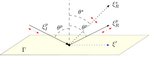 Figure 1
Peer Reviews
No public reviews on file for this paper yet. If you reviewed it on a platform where reviews are public (OpenReview, ICLR, NeurIPS, ICML), you can paste yours below so the community can read it here.
Videos
No videos yet. Explain this paper in a talk, walkthrough, or lecture? Add one.
The transmission problem in linear isotropic elasticity
Plamen Stefanov
Department of Mathematics, Purdue University, West Lafayette, IN 47907
,
Gunther Uhlmann
Department of Mathematics, University of Washington, Seattle, WA 98195, Department of Mathematics University of Helsinki, Finland, IAS, HKUST, Clear Water Bay, Hong Kong, China
and
Andras Vasy
Department of Mathematics, Stanford University, Stanford CA 94305
Abstract.
We study the isotropic elastic wave equation in a bounded domain with boundary with coefficients having jumps at a nested set of interfaces satisfying the natural transmission conditions there. We analyze in detail the microlocal behavior of such solution like reflection, transmission and mode conversion of S and P waves, evanescent modes, Rayleigh and Stoneley waves. In particular, we recover Knott’s equations in this setting. We show that knowledge of the Dirichlet-to-Neumann map determines uniquely the speed of the P and the S waves if there is a strictly convex foliation with respect to them, under an additional condition of lack of full internal reflection of some of the waves.
First author partly supported by NSF Grant DMS-1600327
Second author partly supported by NSF Grant CMG-1025259 and DMS-1265958, and a Simons fellowship
Third author partly supported by DMS-1664683.
1. Introduction
The main goal of this work is to study the transmission problem in isotropic linear elasticity. Let be a smooth bounded domain. Let be closed disjoint smooth surfaces (interfaces) splitting into subdomains with exterior boundary (with ) and interior one , see Figure 1, left. Assume that the density and the Lamé parameters , are smooth up to those surfaces with possible jumps there. We also assume that at at every point, at least one coefficient has a non-zero jump. We impose the following transmission conditions
[TABLE]
where stands for the jump of from the exterior to the interior across any of those surfaces, and are the normal components of the stress tensor, see (2.3). We are motivated by the isotropic elastic model of the Earth where the density and the Lamé parameters jump across the boundary between the crust and the mantle, etc. We study the time-dependent elastic system, see (2.1).
The first goal of this paper is to describe qualitatively the microlocal behavior of solutions of this problem. At any interface , an incoming S or P wave can generate two reflected waves, one S wave and one P wave through mode conversion and two transmitted ones. Then each branch can generate four more, etc., see Figure 1. In some cases, there might be a full internal reflection for one or both of the waves, and there could be no transmitted or reflected waves of a certain kind. In fact, the missing waves would be evanescent modes.
While works on geometric optics for the elasticity system exist (no transmission) [3, 13, 21, 22, 23, 31, 2], a comprehensive analysis of the transmission problem in linear elasticity has not been done to authors’ knowledge. In case of a flat surface and constant coefficients, some cases have been analyzed in the geophysics literature, see, e.g., [19, 20, 1, 25, 26]. In that case, if there is no full internal reflection, one looks for solutions in terms of potentials to reduce the number of variables; and the potentials of the four waves corresponding to an incoming one solve a system which decouples into a and a one, see also (7.5) and (7.6). Those equations were derived by Knott [16] and Zoeppritz [42] more than a century ago, see also [1]. In a recent paper [4], the hyperbolic-hyperbolic (HH) case is analyzed for variable , and but the construction for a curved boundary is partial only. The (HH) case is characterized by the wavefront of the Cauchy data on : it could belong to projected S and P waves on either side of it, and in particular, there are no evanescent modes, see Section 5. This is just one of the many cases since we may have full internal reflection of some or both waves on one or both sides of ; and mode conversion to evanescent modes, see Section 9.3 for a summary. The most general study we are aware of is [40] where the coefficients are constant but cases other than the (HH) one are considered, even though not as extensively as we do it in this paper.
We analyze the general case of variable coefficients and a curved interface in all cases, away from glancing rays. We are interested in two main questions: is the problem well posed microlocally; and (control) can we create every configuration on one side with suitably chosen waves on the other. By doing that, we also compute the principal parts of the reflected and the transmitted waves. The microlocal well posedness reduces to showing the ellipticity of some DO system on with not particularly simple looking entries. Its solution serves as initial conditions for the corresponding transport equations for the hyperbolic of for the evanescent modes. In the flat, constant coefficients case, this system is actually the computation giving us the whole solution. Going back to the general case, in the (HH) microlocal region, we have four outgoing waves, each one being 3D vector-valued. This gives as a DO system for showing-well posedness. If we allow both S and P waves coming from both sides, we would have a system which we want to solve for some group of variables. The control question is reduced to solving the same system with a rearrangement of the unknowns: we are given the waves on one side and want to solve for the waves on the other.
Doing this analysis with brute force does not seem to be a promising approach. Instead, we look for inspiration in the geophysics (and the existing math) literature using the flat constant coefficient case as a starting point. We express the P and the S waves in terms of potentials, as the divergence and as the curl of such potentials on a principal symbol level first; and we extend this to an arbitrary order. We adapt this to the boundary value problem. Having such microlocal mode separation, we also split the S waves in the SV (shear-vertical) and SH (shear-horizontal) waves. This decomposition is valid on only, and depends on the point (and the codirection). Then we reduce those systems to more manageable decoupled plus ones for the outgoing solutions given the incoming ones; their extended versions are plus ones, see (9.12) and (9.13). If the boundary is flat and the coefficients are constant, those are exactly Knott’s equations [16]. Their ellipticity, needed to show well posedness, turns out to be a consequence of energy preservation (even though the determinant can be computed and analyzed [1]), another observation due to Knott. Ellipticity needed to show control can be verified easily and follows from the microlocal well posedness of the boundary value Cauchy problem.
We do this analysis in all microlocal cases with some or even all waves being evanescent; in that case we call them modes. The corresponding matrix symbols do not need to be recomputed; we just need to be careful which imaginary square roots to chose. Ellipticity based on energy preservation needs modifications though. Evanescent waves do not carry (high frequency) energy on the principal symbol level, at least.
We do such analysis for the boundary value problem for the outgoing solutions as well with Dirichlet or Neumann, homogeneous or not, boundary conditions. We also analyze the microlocal boundary value Cauchy problem. We start with the (principally scalar) acoustic equation first for two reasons: it is a needed ingredient in the analysis of the elastic system and SH waves behave as acoustic ones (no mode conversion).
We also study the surface waves propagating along the boundary (Rayleigh waves) or along an internal interface (Stoneley waves). Taylor [35] characterized Rayleigh waves as a propagation of singularities phenomenon when and is flat, and he also mentions that the analysis applies to the general case as well. The existence of such waves is due to lack of ellipticity of the Dirichlet-to-Neumann (DN) operator in the elliptic region on and in the elliptic-elliptic one on an internal interface. Restricted to the surface or , they solve a real principal type of system; and the solution extends as an evanescent one in . Yamamoto [40] viewed Stoneley waves in a similar fashion. A more detailed analysis of the Rayleigh and the Stoneley waves will appear in a work of Y. Zhang.
We also present an application of this analysis to the inverse problem of recovering the coefficients form the outgoing DN map. We recover first the lens relation associated with incoming S and P waves in the first layer ; then we use the recent results by the authors [30] about local recovery of a sound speed (or a conformal factor) from localized travel times. By [2], we can recover in as well, therefore we can recover all three coefficients , and there. In [30] we prove conditional Hölder stability as well which makes this approach for the inverse problem in this paper potentially stable as well; when it can be applied. In the case of no internal interfaces, this was done in [31]. The inverse problem for transversely anisotropic media is studied in [8]. The presence of interfaces however complicates the geometry considerably, see Figure 1 for the recovery of the coefficients in the deeper layers. The lens relation corresponding to a single S or P wave (ray) is multi-valued in general and there is no direct way to tell which branch is coming from which layer, roughly speaking. This makes the inverse problem much different. An essential difficulty following this approach is that there could be totally internally reflected rays in the interior side of one interface which never get out, not even through mode conversion. Then they cannot be generated by rays from the exterior (by “earthquakes”). We show that if there is no total internal reflection of S waves on the interface (from the interior), we can recover below it. This is more general than the result in [4] where , and there is the implicit assumption that there is no full reflection of S and P waves. Since we do not recover all three coefficients below the first interface, we use arguments based on the geometry and the directions of the polarization only, which depend on the speeds only. Next, we also show that if there is no total internal reflection of waves as well, one can recover in . Those arguments can be used to get even deeper into with the appropriate assumptions on the speeds.
2. Preliminaries
2.1. The elastic system
The isotropic elastic system in a smooth bounded domain is described as follows. The elasticity tensor is defined by
[TABLE]
where , are the Lamé parameters. Assume for now that the coefficients , and are smooth in . The elastic wave operator is given by
[TABLE]
where is the density and the vector function is the displacement. The corresponding elastic wave equation is given by
[TABLE]
see, e.g., [26]. The stress tensor is defined by
[TABLE]
Note that , where is the divergence of the 2-tensor .
The Dirichlet boundary condition for is prescribing on the boundary; while the natural Neumann boundary condition is to prescribe the normal components of the stress tensor
[TABLE]
where is the outer unit normal on . This is the operator appearing in the Green’s formula (2.15) for but also has the physical meaning as the infinitesimal deformation of the material in normal direction.
Let be a smooth surface where the coefficients , , may jump. The physical transmission conditions across are the following. First, kinematic ones: the displacements on both sides of should match (no slipping of the material w.r.t. each other); and second, dynamical ones: the normal components on both sides should match (same traction). Therefore, if we declare one side of external and the other one internal, and denote by the jump of across from the exterior to the interior, we obtain the transmission conditions (1.1) on . Note that in , the operator depends on , and and has different coefficients on each side of .
The operator is symmetric on . It has a principal symbol
[TABLE]
which can be also written as
[TABLE]
Taking and , we recover the well known fact that has eigenvalues and with
[TABLE]
of multiplicities and and eigenspaces , and , respectively. We have . Those are known as the speeds of the P waves and the S waves, respectively. The eigenspaces correspond to the polarization of those waves. The characteristic variety is the union of and , each one having two connected components (away from the zero section), determined by the sign of .
Let solve the elastic wave equation
[TABLE]
with given so that for and all coefficients smooth in (no transmission interfaces). The (outgoing) Dirichlet-to-Neumann map is defined by
[TABLE]
see (2.3), where is the outer unit normal on , and is the stress tensor (2.2).
2.2. An invariant metric based formulation
We have
[TABLE]
where we sum over repeating indices even if they are both lower or upper. This can also be written in the following divergence form
[TABLE]
where is the symmetric differential, and is the divergence of symmetric fields with the adjoint in sense.
To prepare ourselves for changes of variables needed in the analysis near surfaces that we will flatten out, we will write in an invariant way in the presence of a Riemannian metric . We view as an one form (a covector field) and we define the symmetric differential and the divergence by
[TABLE]
where is the covariant differential, , is a covector field, and is a symmetric covariant tensor field of order two. Note that increases the order of the tensor by one while decreases it by one. Then we define by (2.10). We still have , where the adjoint is in the space of contravariant tensor fields, see, e.g., [24].
The stress tensor (2.2) is given by
[TABLE]
and then . The Neumann boundary condition at is still given by prescribing the values of on it as in (2.8). The operator , defined originally on extends to a self-adjoint operator in . This extension is the one satisfying the zero Dirichlet boundary condition on . In particular, this shows that the mixed problem (2.7) is solvable with regular enough data at least since one can always extend inside and reduce the problem to solving one with a zero boundary condition and a non-zero source term; and then use the Duhamel’s principle for the latter.
The principal symbol of in the metric setting is still given by (2.4) with the proper interpretation of the dot product there:
[TABLE]
where as usual. In particular, the speeds and remain as in (2.6). The eigenspaces of the symbol are still and , the latter being the covectors normal to . Notice that under coordinate changes, the coordinate expression for changes as well, as a covector.
We recall that the cross product on an oriented three dimensional Riemannian manifold is defined in the following way. If and are covectors at some fixed point , then is defined as the unique covector satisfying
[TABLE]
where is the metric inner product of covectors, and is the volume form on the tangent bundle. To compute it in local coordinates, let . Then we get
[TABLE]
where the latter is the determinant of the matrix with the indicated columns (also, the Euclidean volume form of them). Therefore, equals the Euclidean cross product
[TABLE]
This yields
[TABLE]
Similarly, the curl of a covector field is defined as the Hodge star of the exterior derivative , and we have
[TABLE]
The divergence of is given by and in particular, . We will use the notation for as well.
One can verify that the double vector product of two covectors in the metric still satisfies , as in the Euclidean case.
2.3. Existence of dynamics
We assume now, as in the rest of the paper, that can be expressed as a union of layers as explained in the Introduction and , and are smooth up to their boundaries with possible jumps at them. We also assume that is the metric based operator (2.10).
Lemma 2.1**.**
Let be as above. Then , defined originally on functions smooth up to and , satisfying the transmission conditions (1.1), and zero boundary conditions on , extends to a self-adjoint operator in .
Proof.
We start with Green’s formula. Let be a bounded domain with a smooth boundary so that are smooth in . Then
[TABLE]
where is the area measure in induced by . To prove it, write
[TABLE]
since . The last integral equals
[TABLE]
Switch and and subtract the resulting formulas to prove (2.15).
Assume now that and are smooth up to the interfaces, may jump there and satisfy the transmission conditions (1.1). We apply (2.15) to , , …, and sum up the results. Note that the outer normal to at is the inner one at the same when viewed from , etc. As a result, we get (2.15) in as well, despite the discontinuities because by the transmission conditions (1.1), all contributions from cancel. By the zero boundary condition on , the r.h.s. of (2.15) vanishes. Therefore, is symmetric.
To show that there is a natural self-adjoint extension, it is enough to show that the quadratic form is bounded from below. For every smooth satisfying the Dirichlet boundary condition, by (2.10) we have
[TABLE]
which is non-negative.
We can write the Cauchy problem at for (2.1) with Dirichlet boundary conditions now as
[TABLE]
The operator is self-adjoint on the energy space with norm
[TABLE]
Then by Stone’s theorem, the Cauchy problem at for (2.1) with Dirichlet boundary conditions is solved by a unitary group. Problem (2.7) can be solved for regular enough by extending inside and reducing it to a problem with a source but with homogeneous Dirichlet boundary conditions; and solving it by Duhamel’s formula. ∎
2.4. The Neumann boundary operator
Let be semigeodesic coordinates to a given surface , with on one side of it, defining the orientation in the metric setup. The metric then takes the form in those coordinates with for . Then, see also [31],
[TABLE]
Therefore,
[TABLE]
where and we used the fact that .
3. Geometric optics for the wave equation with DO lower order terms
We recall the well known geometric optics construction for a hyperbolic pseudo-differential equation generalizing the acoustic wave equation, see, e.g., [36, 37]. We allow the equation to be a system but we still assume that the principal part is scalar, see also [9]. In this generality, the construction is done in [36, VIII.3]. We are not going to formulate results about the propagation of the polarization set which can be derived from [9]. The reason to do study the acoustic equation in this generality is two-fold. First, the elastic system decomposes into such pseudo-differential equations; and second, SH waves propagate like acoustic ones as we show below.
3.1. The Cauchy Problem with data at
Our interest is in the acoustic wave equation with lower order classical pseudo-differential term
[TABLE]
with Cauchy data at . Here, is a Riemannian metric that we include in order to have the flexibility to change coordinates easily; and is the Laplace-Beltrami operator. The distribution is vector valued and is a matrix valued DO. Up to lower order terms, coincides with . The characteristic variety is given by and has two connected components corresponding to and , away from the zero section (notice the convention that corresponds to ). We are looking for solutions of the form
[TABLE]
modulo terms involving smoothing operators of and , defined in some neighborhood of , with some . This parametrix differs from the actual solution by a smoothing operator applied to , as it follows from standard hyperbolic estimates. The signs correspond to solutions with wave front sets in , respectively as it can be seen by applying the stationary phase lemma.
Here, are classical amplitudes of order zero depending smoothly on of the form
[TABLE]
where is homogeneous in of degree for large . The phase functions are positively homogeneous of order in solving the eikonal equations
[TABLE]
Such solutions exist locally only, in general. While the principal symbol is the only one determining the eikonal equations and therefore the geometry, the subprincipal symbol in (3.1) depending on the principal one of , affects the leading amplitude below.
Since the principal symbol of the hyperbolic operator in (3.1) allows the decomposition , in a conic neighborhood of , one can apply a parametrix of to write (3.1) there as
[TABLE]
with of order zero and being the sum of the terms in (3.2). This is the case studied in [36, VIII.3] with a more general elliptic replacing , allowing to be a vector function, and to be matrix valued.
The main tool is the “fundamental lemma” allowing us to understand the action of a DO on in terms of a homogeneous expansion in , see [36, VIII.7] and [38]. The lemma remains true for principally scalar systems and it is used for such in [36].
We recall the construction of the amplitude. Let be as the first term in (3.2) with the indices there dropped, corresponding to . We seek the amplitude of the form as in (3.3) but the upper index is a lower one now.
The order two terms in the expansion of cancel because solves the eikonal equation (3.4) with the plus sign. Equate the order terms, we must solve
[TABLE]
where is the expansion of and they are evaluated at . In our case, , therefore, , which for yields . Therefore, the vector field in (3.6) is proportional to the vector field which is the Hamiltonian covector field of the wave equation (3.1) on identified with a vector one, since the Laplacian there is the one associated with the metric . As it is well known, this is also the geodesic vector field of in the tangent bundle. The potential-like term in (3.6) involves , see (3.5). Now, the transport equation (3.6) is a first order linear ODE along the bicharacteristics for the vector valued with a matrix valued zero order potential-like term. Given initial conditions at , it is solvable as long as is well defined.
The higher order transport equations for , , etc., are derived in a similar way. They are non-homogeneous, with the same left-hand side but on the right we have functions computed in the previous steps.
We return to (3.2) now and look for as a sum of four terms as indicated here, each one of the type we described. We can use the Cauchy data to derive initial conditions for the transport equations, see e.g., [28], to complete the construction.
The integrals appearing in (3.2) are Fourier Integral Operators (FIOs) either with considered as a parameter, or as considered as one of the variables. In the former case, singularities of propagate along the zero bicharacteristics. More precisely, for every ,
[TABLE]
where , and
[TABLE]
and for , is the geodesic issued from in direction .
On the other hand, considering as one of the variables,
[TABLE]
where
[TABLE]
In the analysis below, we will consider only.
The construction above can be done in some neighborhood of a fixed point in general. To extend it globally, we can localize it first for with in a conic neighborhood of some fixed . Then will be well defined near the geodesic issued from that point but in some neighborhood of in general. We can fix some at which is still defined, take the Cauchy data there and use it to construct a new solution. Then we get an FIO which is a composition of the two local FIOs each one associated with a canonical diffeomorphism, then so is the composition. Then we can use a partition of unity to conclude that while the representation (3.2) is local, the conclusions (3.7) and (3.8) are global. In fact, it is well known that both and with fixed are global FIOs associated with the canonical relations in (3.7) and (3.8).
In particular, if is a smooth hypersurface, and hits for the first time transversely locally, then is an FIO again with a canonical relation as above but with and replaced by its tangential projection . Notice that for and for . Also, with equality for tangent rays that we exclude; therefore, is in the hyperbolic region, as defined below.
3.2. The boundary value problem for the acoustic equation
Let be a smooth hypersurface near a fixed point given locally by . We take to be local semigeodesic coordinates. We define to be the “positive” and the “negative” sides of . At the beginning, we work in only and omit the superscript or the subscript from the corresponding quantities. For all possible solutions (not restricted to incoming or outgoing ones) with singularities not tangent to , we want to understand how the Dirichlet data and the Neumann data are related. Once we have this, we can understand microlocally the boundary value problems with either Dirichlet or Neumamn boundary conditions, or with Cauchy data.
The analysis depends on where the wave front set of the Cauchy data is. Let be supported near some . Then has a natural decomposition into the hyperbolic region , the glancing one , and the elliptic one . Each one has two disconnected components corresponding to . We will recall the analysis in the component in more detail and will point out the needed changes when . Also, we will not analyze (a neighborhood of) the glancing region; for that, see, e.g., [36] for a strictly convex boundary. We are looking for a parametrix of the outgoing solution of (3.1) with boundary data , i.e., the solution with singularities propagating in the future only. Solutions with singularities propagating to the past only will be called incoming.
3.2.1. The outgoing and the incoming Neumann operators
If is the outgoing solution with boundary data with in the hyperbolic region, we call the operator the outgoing Neumann operator. Similarly we define the incoming Neumann operator by . In those definitions, it is implicit that the solutions are defined in and is the unit normal exterior to it. i.e., . If we have as above, we use the notation , to denote the four Neumann operators with the convention that we preserve for , i.e., is interior for it. If the coefficients of the wave equation are smooth across , we have , up to smoothing operators. In the transmission problem below however, this is not the case.
3.2.2. Wave front set in the hyperbolic region
Assume that is in the hyperbolic region with . We are looking for a representation of of the form
[TABLE]
with a phase function and an amplitude .
The phase function solves the eikonal equation in (3.4) with the plus sign but with a boundary condition on the timelike boundary now
[TABLE]
The choice of the positive square root reflects the assumption . In the hyperbolic region, there are two solutions depending on the choice of the sign of at . It is easy to see that what corresponds to outgoing solutions is the positive choice
[TABLE]
We solve (3.10) with this condition locally. To construct the amplitude, we solve the same transport equations (3.6) as above but with initial condition for , i.e., the principal part of is one there; and all others vanish.
The case is similar: we seek the solution in a similar way but the sign in (3.10) is negative. This does not change the construction.
Incoming solutions are constructed similarly. We choose the negative square root in (3.11). in particular we get that the outgoing and the incoming Neumann operators are DOs of order one with principal symbols equal to multiplied by (3.11), see also Proposition 3.1 below.
3.2.3. Wave front set in the elliptic region . Evanescent waves
We proceed formally in the same way but the problem here is that the eikonal equation has no real valued solution because the expression under the square root in (3.11) is negative. It may not even have a complex valued solution. This is a well known case of an evanescent mode described by a complex valued phase function (and amplitude). We follow [11], see also [36, VIII.4]. Since the construction in [11] is done for the Helmholtz equation with a large parameter and in [36, VIII.4] it is done for an elliptic boundary value problem, respectively, we need to do them in our hyperbolic case as well, even though the construction is essentially the same. We assume that belong to a conically compact neighborhood, contained in the elliptic region, of a fixed point there. Plugging the ansatz in the elasticity equation, we use the “fundamental lemma” for complex phase functions in [38, X.4] to get an asymptotic expansion which formally look the same as in the hyperbolic case. We are looking for a solution of the eikonal equation (5.1) for up to an error at as a formal infinite expansion of the form
[TABLE]
where are symbols of order . We denote this class by , and by replacing the order by some , we denote by the corresponding class. To avoid exponentially large modes, we require . To construct the formal series, we first write the eikonal equation (3.11) in the form
[TABLE]
(note that there are no incoming/outgoing choices here) and then differentiate it w.r.t. at . If such a solution exists, the error term would not affect those derivatives. We have
[TABLE]
To find the higher order derivatives, we write (3.12) in the form
[TABLE]
with homogeneous in of order one. Then
[TABLE]
Since is a symbol of order one, we prove the claim. Note also that .
The next step is to solve the transport equations. Since they have complex coefficients, they may not be solvable exactly and we solve them up to an error as well. The rest is as in [11] and [36, VIII.4].
Proposition 3.1**.**
In the hyperbolic region, and are DOs of order one with principal symbols
[TABLE]
In the elliptic one, they are DOs of order one again with principal symbols
[TABLE]
We recall that in the coordinates we used to compute the principal symbols. The expressions we got are invariant however. In both cases, the DN maps are elliptic. As shown in [36], they are elliptic even in the glancing region but they belong to a different class of DOs. The principal symbols of the Neumann operators on the negative side are similar but with opposite signs.
3.2.4. The boundary value problem with Dirichlet data
The problem of constructing the outgoing solution with Dirichlet data on was solved above when is either in the hyperbolic of the elliptic region. Similarly, we construct . Notice that in the elliptic region, the construction is the same for both. In particular, we proved Proposition 3.1 by taking the normal derivatives of those solutions.
Next, we can construct a reflected wave. Assume we have an incoming solution with singularities hitting transversely. We want to construct a solution equal to for satisfying on the boundary. Then has a wave front set in the hyperbolic region only. We construct the reflected wave as the outgoing solution with Dirichlet data . Then is the solution we seek.
3.2.5. The boundary value problem with Neumann data
Consider the outgoing solution with boundary data on . We reduce it to the Dirichlet problem above by inverting the DN map in . Since the latter is elliptic in the two regions we work in, this can be done microlocally. Then we solve a Dirichlet problem. We do the same for the incoming solution.
If we want to construct a reflected wave so that the solution satisfies , we need to solve which is possible since is elliptic. Having , then we construct the outgoing solution with that Dirichlet data.
3.2.6. The boundary value problem with Cauchy data
We are looking for a microlocal solution of the acoustic equation (3.1) satisfying and on with given and having wave front sets in the hyperbolic region first. The global Cauchy problem is over-determined because the singularities can hit the boundary again and therefore the Cauchy data have a structure (consisting of pairs in the graph of the lens relation); therefore prescribing them arbitrarily is not possible. On the other hand, one can construct a microlocal solution locally, when the wave front sets of and are localized in small conic sets excluding tangential directions, until the singularities hit the boundary again. We are looking for as a sum of two solutions , one incoming and the other one outgoing. To determine the boundary values of the two solutions and to reduce the problem to section 3.2.4, we need to solve
[TABLE]
where and are the boundary values of those solutions.
Let be in the hyperbolic region first. Then on principal symbol level, the leading amplitudes solve
[TABLE]
where is defined by (3.11). This in an elliptic system. This shows that the matrix valued operator in (3.16) is elliptic (if we reduce the order of the second equation to [math] by applying an elliptic DO of order ). Therefore, the Cauchy data determine uniquely a decomposition into an incoming and an outgoing solution, locally. This reduces the problem to the one we solved in section 3.2.
If is in the elliptic region, there is only one parametrix, no incoming or outgoing ones. The corresponding DN map is an elliptic DO of order one with principal symbol (3.15). Then for to be Cauchy data of an actual solution (up to smooth functions) it is needed that it belongs to the range of (up to smooth functions). This makes this problem over-determined. If , a microlocal solution exists, as we showed above. It propagates no singularities away from , and it does not propagate singularities along either (unlike the Rayleigh waves in elasticity which propagate along ).
3.3. The transmission problem
We recall the setup in section 3.2. We work locally in a small neighborhood of a point on and call one of its sides, negative, the other one, , positive. For the speed , we have in , and in , where are smooth up to and pointwise. We impose the transmission conditions
[TABLE]
where is the normal derivative. Let be semi-geodesic coordinates near so that in .
Let be an incident solution of the acoustic equation (3.1) with speed and background metric with a wave front set localized near a small conic neighborhood of some covector (at some time) approaching from the positive side. As mentioned above, we consider singularities which move in the direction of only, i.e, associated with in (3.2), as we did in section 3. Then on , with considered as a variable, we have . Extend the speed form the negative to the positive side in a smooth way (recall that jumps across ) and extend smoothly across as a solution with that speed. Set
[TABLE]
Let with be one of the singularities of . We assume that is a unit covector w.r.t. . We have that is in the hyperbolic region in . We are looking for a parametrix near of the form
[TABLE]
where is incoming and restricted to ; is the reflected outgoing solution supported in , and is the transmitted outgoing one or an evanescent mode, supported in . It is enough to find the boundary values of those functions.
3.3.1. The hyperbolic-hyperbolic case
Assume that is in the hyperbolic region in as well, i.e., on . If at (transmission from a fast to a slow region), that condition is satisfied regardless of . If (transmission from a slow to a fast region), existence of a transmitted ray depends on . Let be the angle which an incoming ray makes with the normal, then the reflected angle will be the same and the angle of the transmitted ray, see Figure 2, is related to by Snell’s law
[TABLE]
which follows directly from (3.10) with and there, see also [29]. This relation shows that a transmitted ray will exist only if does not exceed the critical angle
[TABLE]
The transmission conditions (3.17) are equivalent to
[TABLE]
Assume now that we want to satisfy transmission conditions requiring continuity of and its normal derivative across the boundary. Then we get the following linear system for the leading terms and of the amplitudes and :
[TABLE]
where
[TABLE]
In particular, this shows that the determinant of (3.23) is negative, and therefore, the system is solvable, i.e., elliptic after reducing the order of the second equation to zero. Since the system (3.22) is elliptic, it can be solved up to infinite order, i.e., we can find the all terms at . The solutions serve as initial conditions for the transport equations of the corresponding modes.
Multiplying the first by the conjugate of the second equation, we get
[TABLE]
which can be considered (and justified) as preservation of the energy across .
3.3.2. Total internal reflection
Assume now that is in the elliptic region for . This happens when . In that case, there will be no transmitted singularity. Indeed, we are looking for an evanescent mode in . Then in (3.22) is in the elliptic region. The analog of (3.23) then is
[TABLE]
where is pure imaginary and given by (3.15) times . Equivalently,
[TABLE]
Take the real part of the first equation multiplied by the conjugate of the second one to get
[TABLE]
In other words, on principal level, the whole energy is reflected and nothing is transmitted. We could have obtained this directly by solving (3.25), of course.
3.3.3. Incoming waves from both sides of .
A more general setup is to assume incoming waves from each side, see Figure 2, right. We do not need to assume hyperbolic ones; they could be evanescent. In fact, this is an analogue of the Cauchy data case in the boundary value problem, see section 3.2.6. The point of view we adopt and will keep in the elastic case, is to classify the cases by the wave front set of the Cauchy data on the boundary.
We are interested in two questions: (i) well posedness of the transmission problem: given all incoming waves, is the problem well posed for the outgoing ones; and (ii) given all waves on one side of , can we solve for all waves on the other one? We show that (i) is true as it can be expected (and well known). The answer to (ii) is not always affirmative; and when it is; this means that we can control the configuration on one side from the other one; in particular we can kill either the incoming or the outgoing wave on that side.
The hyperbolic-hyperbolic case. We assume now that the Cauchy data (the same on both sides by the transmission conditions) has a wave front set in the hyperbolic region on each side of . Then on each side, we have two solutions: one incoming and one outgoing. Let and be the two incoming solutions from the positive and from the negative side, respectively, and let , be the two outgoing ones. A usual, we assume no tangent rays. Then the transmission conditions are given by
[TABLE]
This is a generalization of (3.22) with one more wave added. If the corresponding principal amplitudes are , , , , we get
[TABLE]
Clearly, each matrix is elliptic. This implies that we have control from each side: given any choice of two amplitudes on one side, say , one gets an elliptic problem for finding the amplitudes on the other one, in this case .
We also get ellipticity for solving for the outgoing/incoming waves given the incoming/outgoing ones, i.e., the transmission problem is well posed. This also follows from energy conservation. Indeed, multiplying the first by the conjugate of the second equation, and then taking the real part above yields
[TABLE]
This energy preservation across the boundary implying in particular that if all incoming waves vanish, then so do the outgoing ones; i.e., that problem is elliptic.
The hyperbolic-elliptic case. We assume now that the Cauchy data (the same on both sides by the transmission conditions) has a wave front set in the hyperbolic region w.r.t. and in the elliptic one for . Then in we have two solutions: one incoming and one outgoing but in there is only one (evanescent) solution. This case is analyzed in section 3.3.2 with , , (no incoming or outgoing ones) corresponding to there. We found out there that the incoming wave (or the outgoing one) determines uniquely the outgoing (respectively, the incoming) one and the evanescent one . On the other hand, we cannot control and by choosing appropriately the evanescent mode appropriately; in fact alone determines the whole configuration already.
A slightly different point of view into this case is that we cannot have arbitrary (up to smooth functions) Cauchy data on in the hyperbolic region for , since that data falls in the elliptic region on the negative side, and then it has to be in the graph of the Neumann operator . On other hand, if that data satisfy that compatibility condition, the solution in consists of an incoming and a reflected wave. This is in contrast to the hyperbolic-hyperbolic case, where we can cancel one of the waves on the top, for example.
The elliptic-elliptic case. We assume now that the Cauchy data has a wave front set in the elliptic region w.r.t. both and . It is interesting to see if we can have evanescent modes on both sides but still a non-trivial wave front set on . We would need which cannot happen. Therefore, there are no Rayleigh or Stoneley kind of waves in the acoustic case.
3.4. Justification of the parametrix
In each particular construction up to section 3.2.6, we constructed a parametrix satisfying the equation and the corresponding initial/boundary conditions up to a smooth error. Then the difference of the parametrix and the true solution satisfies all those conditions up to smooth errors. Standard hyperbolic estimates imply that the difference is smooth. In section 3.2.6, the Cauchy problem on a timelike boundary needs to be solved microlocally only and it is a tool to handle the transmission one. The justification of the parametrix for the latter can be done with the aid of [12, 39], guaranteeing smooth solutions if the transmission conditions (1.1) hold up to a smooth error only.
4. Geometric optics for the elastic wave equation
We study the Cauchy problem at and propagation of singularities in the elastic case. We present the geometric optics construction for the elastic wave equation in an open set first, where the coefficients are smooth. Such a construction is well known for systems with characteristics of constant multiplicities, see, e.g., [36, 37] and [9]. Our goal is to make the elastic case more explicit and to do a complete mode separation which we will use eventually near a boundary, see Proposition 4.1 below. The elastic case has been studied form microlocal point of view in [40, 21, 22, 23, 13, 3, 31].
Consider the elastic wave equation
[TABLE]
with Cauchy data at . We want to solve it microlocally for in some interval and in an open set. The operator is associated with a Riemannian metric as in section 2.2. If , and are constant and Euclidean, one can use Fourier multipliers. In that case, let be the projection to the p-modes, i.e., is the Fourier multiplier and let . It is easy to see that is the Fourier multiplier . Also, we may regard as the potential/solenoidal (or the Hodge) decomposition of the 1-form , see, e.g., [24]. Then , . We have a complete decoupling of the system into P and S waves.
In the variable coefficient case, we will do this up to smoothing operators. We recall the construction in [36], which provides another proof of the propagation of singularities in this case. The principal symbol of has eigenvalues of constant multiplicities. Near every , one can decouple the full symbol fully up to symbols of order . Namely, there exist an elliptic matrix valued DO of order [math] microlocally defined near , so that
[TABLE]
modulo near , where the matrix is in block form; with an block on the lower right and a one on the upper left ( is actually with being the identity in two dimensions). Moreover, and are DOs of order one. In other words, the top non-zero block is scalar and the lower non-zero one is principally scalar. We recall this construction briefly. We seek as a classical DO with a principal symbol which diagonalizes ; there are many microlocal choices, and we fix one of them. Then
[TABLE]
where is of order one. Then we correct by replacing it with with some DO of order , i.e., we apply to the right and to the left to get
[TABLE]
where we used the fact that mod . Let us denote the matrix operator there by . To kill the off diagonal terms on the right up to zeroth order, we need to do that for . Note that and do not commute up to a lower order because they are matrix valued DOs. We look for in block form with zero diagonal entries and off-zero ones (an vector) and (a vector). If we represent in a block form as well, we reduce the problem to solving
[TABLE]
modulo . The solvability of this system on a principal symbol level follows by the general lemma in [36, IX.1] because but in this particular case, it is straightforward. Note that the principal symbols of and represent the coupling of the P and the S waves on a sub-principal symbol level, see also [3].
We apply to the left and to the right to kill the off diagonal terms of , etc. In fact, can be chosen to be unitary in microlocal sense [27]. In our case however, we prefer to be of order one.
From now on, we will do all principal symbol computation at a fixed point where is transformed to an Euclidean one (via the exponential map, for example) to simplify the notation. Then we will interpret the final result in invariant sense.
The principal symbol, of , at that fixed point, will be chosen to be
[TABLE]
when . The third column is the eigenvector associated with , while the first and the second ones are a basis of the eigenspace of associated with ; and that basis is (micro) local only. In fact, a global one does not exist since those vectors are characterized as being conormal to . In this particular case, we chose and with , etc.
Recall that the principal symbol computations so far are at a single point where is Euclidean. To extend it to all points, an invariant way to choose is to replace the first and the second column there by and with considered as covectors, and the cross product as in (2.13). In other words, the first two columns in (4.5) are considered as vectors, then converted to covectors by the metric and multiplied by . Then we still get (4.9) but in we have curl in terms of the metric, see (2.14).
It then follows that microlocally, the elasticity system can be written as for
[TABLE]
where and is scalar. This system decouples into the wave equations
[TABLE]
with of order one, smoothing; the first one is a system and the second one is scalar. The first one has as a characteristic manifold, while the second one has . Even though depends on the microlocal neighborhoods of the characteristic varieties we work in, the wave front sets of , in those neighborhoods, we can apply the propagation of singularities results, or directly the microlocal geometric optics construction used below. Then we conclude that singularities in those neighborhoods propagate along the zero bicharacteristics of and , respectively (which, of course, is well known). This implies a global result, as well.
For we get
[TABLE]
where and have wave front sets in and , respectively. We call such solutions microlocal S and P waves. We have
[TABLE]
where and are of order zero and are formed by the lower order entries of . Here can also be written as .
Therefore, we proved the following.
Proposition 4.1** (mode separation).**
Let be a solution of the elastic wave equation in the metric setting in some open set in . Let and be microlocalized near and , respectively. Then, microlocally, in any conic subset where , there exist a scalar function and a vector valued function solving (4.7) so that , where
[TABLE]
with and DOs of order zero and the curl in is in Riemannian sense.
The assumption does not restrict us. We can always rename the variables or rotate the coordinate system. On the other hand, the proposition does not provide a global mode separation. We are going to use it with being the distance to the boundary. Note also that and , are related by (4.6).
In the geophysics literature, and such that (in our case, ) are called potentials. We have some freedom to choose so that (4.10) hold: adding an exact form to would not change the principal part of at least. One possible gauge to get unique is to take one of the components, in some coordinate system, to be zero. We have in (4.10). The analysis however must be restricted microlocally to . In what follows, will be the normal coordinate to the boundary. Another choice is to require to be solenoidal, i.e., divergence free.
This proposition is a generalization of the well known representation of the solution of the isotropic constant coefficient elastic equation into potentials solving (4.7) with the operators and there vanishing. To guarantee uniqueness, it is often assumed that , . We can prove a version of this in the variable coefficient case as well.
5. The boundary value problem for the elastic system. Dirichlet boundary conditions
Consider the elastic wave equation with boundary data on . Assume that for and we are looking for the outgoing solution, i.e., the one which vanishes for . We also introduce the notion of a microlocally outgoing solution along a single bicharacteristic requiring singularities of such a solution to propagate to the future. We define similarly incoming solutions by reversing time. Note that an outgoing solution does not need to consist of microlocally outgoing ones only since some incoming ones may be canceled at interfaces by outgoing ones. We will construct a parametrix of those solutions using the analysis in section (3.2). Moreover, we study the Cauchy data problem as well. We will use the analysis in the acoustic case essentially.
We work in semigeodesic coordinates , with in . We denote the dual variables by . The Euclidean metric then takes the form in those coordinates with for . The analysis however works if we start with an arbitrary metric in , not just with the Euclidean one. Norms and inner products below are always in the metric or (for covectors).
The phase space on the cylindrical boundary can be naturally split into the following regions (recall that ):
**Hyperbolic region: **
. Then as well, so it is hyperbolic for both speeds.
**P-glancing region: **
. It is glancing for and hyperbolic for .
**Mixed region: **
. It is elliptic for but hyperbolic for .
**S-glancing region: **
. It is glancing for and elliptic for .
**Elliptic region: **
. Then , as well, so it is elliptic for both speeds.
We will not analyze wave fronts in the two glancing regions and . For the purpose of the inverse problem, it is enough to analyze the propagation of singularities away from a set of measure zero. Therefore, there is no need to build a parametrix near the glancing regions (as in [32] or [41], for example) or work as in [12]; so we can avoid the glancing regions.
By the calculus of the wave front sets, the traces of microlocal P waves on have wave front sets in the hyperbolic region under the assumption that all singularities hit the boundary transversely. The traces of transversal microlocal S waves belong to , i.e, either to the hyperbolic, the mixed one, or to the p-glancing one. In particular, the trace of any solution of the elastic system with singularities hitting transversely, has wave front disjoint from the elliptic region. On the other hand, boundary values of solutions of the boundary value or the transmission problem may have wave front set on that surface, as Rayleigh and Stoneley waves do.
The analysis we have done so far, see next section, allows us to decouple the P and the S modes on the boundary completely by their polarizations. Then in terms of the potentials and , we can think of the system as a decoupled one. When modes hit a free boundary, or a transparent one, however, the reflected and the transmitted modes may change type. The reason for this is that the boundary trace of an incoming S or P wave does not belong to the same subspace as that of an outgoing one.
5.1. Wave front set in the hyperbolic region
Let be supported near some , where represents , flattened. Assume first that is supported in the hyperbolic region. The later has two disconnected components determined by the sign of there. Let us assume that is contained with the one with ; the case is similar. Then the characteristic varieties reduce to and , respectively. We are looking for a parametrix of the outgoing solution of the form as in (4.8) with a potential. Note that this construction excludes , which in our case corresponds to tangent rays which we avoid. We will work in a conic open microlocal region which does not contain such rays, i.e., there.
We seek the potentials and as geometric optics solutions as in section 3.2, i.e., of the form (3.9) (where the solution is called , not ) with phases and , respectively, and a scalar amplitude and a 2D vector-valued one . The phase functions solve the eikonal equations
[TABLE]
and similarly for , where . The choice of the positive sign in front of the square root in the eikonal equation is determined by the choice . By (4.10), the principal part of the amplitude of is and that of is . Restricted to the boundary, we have , , where
[TABLE]
We will use the notation
[TABLE]
Those are the codirections of the rays emitted from the boundary, see Figure 3. The angles and with the normal satisfy Snell’s law
[TABLE]
as it follows directly from (5.2), see also [29].
As we stated above, we are going to do all principal symbol calculations at , where can always be arranged to be Euclidean.
In the hyperbolic region we work in, the expressions under the square roots are positive. The positive square roots guarantee that the singularities are outgoing. We determine next the boundary conditions for the transport equations. Since , the boundary values of can be obtained from those of given by by an application of a certain DO. By the “fundamental lemma”, see [36, VIII.7] and [38], near the boundary is given by an oscillatory integral of the type (3.9) with the amplitude there multiplied by a classical symbol with principal part , where equals either or depending on which components of we take. Restricted to the boundary, we get
[TABLE]
with a classical DO on with principal symbol
[TABLE]
The subscript “out” is a reminder that we used the outgoing solution to define . Similarly, we define using the incoming . Its principal symbol is as above but with and having opposite signs. Note that acts locally in while the two new operators act on . The symbol is elliptic, in fact
[TABLE]
which also equals . The inverse of is easy to compute and we do that below. To find the boundary conditions for , we write (recall that all our inverses are parametrices). Then for and we get (4.9) with in all symbols replaced by for and for . Once we have the boundary conditions for , we construct near the boundary by the geometric optics construction (3.9). To get , we apply to the result, see (4.8).
Remark 5.1**.**
In [23], Rachele showed that when is Euclidean, the leading amplitudes (polarizations) of and are independent of if we think of the three parameters being instead of . We will use this in Section 10.
In what follows, we will make the calculations above more geometric. By (4.10), and have representations of the kind (3.9) with the corresponding phase functions and matrix valued amplitudes having principal parts and , where is a vector, and is a matrix. Then one can show that on the boundary, is the non-orthogonal projection to the plane parallel to , and is the non-orthogonal projection to parallel to the latter plane. In other words, they are the projection operators related to the direct sum .
Finally in this section, we notice that the same analysis holds for the incoming solutions with given Dirichlet boundary data. Then in the formulas above, we have to take the negative square roots of and in (5.2).
5.2. Wave front set in the mixed region
Let be in the mixed region next. We show below that the outgoing solution has a microlocal S wave only. The eikonal equation for still has the same real valued solution locally, corresponding to the outgoing choice of the solution . On the other hand, the eikonal equation (5.1) for has no real solution. Indeed, we have on and there is no real-valued function that could solve (5.1) and have such a gradient because in (5.2), would be pure imaginary. This is the case of an evanescent mode described in Section 3.2.3.
We are still looking for a solution of the form but this time , and therefore, is an evanescent mode as the one constructed in Section 3.2.3. The eikonal equation for implies, see (3.13), that in this case reduces to
[TABLE]
Then as in (5.5), (5.6), applying the “fundamental lemma” for FIOs with a complex phase, see [38, X.4], we deduce as before that the boundary values for are given by (5.5) with a classical DO having principal symbol as in (5.6) (with the new pure imaginary ). The operator is still elliptic because the determinant (5.7) has non-zero imaginary part. Then we can determine the boundary conditions for and , construct the microlocal solutions, and apply to get .
5.3. Wave front set in the elliptic region
Assume that is in the elliptic region. Then we proceed as before, looking for both and as evanescent modes with complex phase functions. In this case, both and are pure imaginary with positive imaginary parts, see (5.8), and for we get
[TABLE]
We have
[TABLE]
Therefore, is elliptic and we can proceed as above and construct the solution as in Section 3.2.3.
5.4. Summary
We established that the Dirichlet problem is well posed microlocally and we have the following:
- (i)
in the hyperbolic region: there are outgoing P and S waves.
- (ii)
in the mixed region: there is an outgoing S wave only (plus an evanescent P mode).
- (iii)
in the elliptic region: there are no outgoing waves; there are two evanescent modes.
6. The boundary value problem for the elastic system. Neumann boundary conditions and the Neumann operator
Assume now that we want to find the outgoing solution of the elastic wave equation with boundary data . The strategy below is find the Dirichlet boundary data from this equation and then to proceed as in section 5. In other words, we want to solve for microlocally if possible by showing that is elliptic (or not). Lack of ellipticity of in the elliptic region leads to Rayleigh waves, see, e.g., [5, 35, 33, 32].
6.1. Wave front set in the hyperbolic region
We are looking again for an outgoing solution of the type as in (4.8). The boundary values of are computed by solving
[TABLE]
for , compare with (5.5), where is the microlocalized Dirichlet-to-Neumann map (2.8), i.e., for an outgoing microlocal solution of the elasticity equation with boundary data on . We can use (6.1) and (5.6) to compute .
We define the incoming in a similar way as in (6.1) but with being the incoming solution. More precisely, is defined as where is the incoming solution with boundary data . This also means that , where is defined as with being the incoming solution. The operator the should be denoted by but we will keep the simpler one . Below, we compute the principal symbols of and . Combining that with (5.6), we can compute the principal symbol of as well but we will not need it.
By (2.16) and (5.6), in semigeodesic coordinates,
[TABLE]
Therefore,
[TABLE]
Similarly, we define to be the principal symbol of the same operator but related to the incoming DN map; i.e., the same as above but with and the negative square roots in (5.2).
A direct computation yields
[TABLE]
The determinant of is the same. Since is elliptic, we get that is elliptic in the hyperbolic region as well. Therefore, we can invert microlocally and reduce the Neumann boundary value problem to the Dirichlet one, which can be solved as in section 5.1. More directly, we invert and we get boundary conditions for ; which we use to solve the problem.
6.2. Wave front set in the elliptic region.
In this case, we seek both and as evanescent modes. The calculations are as in section 5 but and are pure imaginary as in (5.8) and (5.9). Then
[TABLE]
We have . For the third factor above, introduce the function
[TABLE]
Then, up to an elliptic factor, equals . It is well known and can be proven easily that on the interval , this function has a unique simple root . This corresponds to . Therefore, if we set , known as the Rayleigh speed, we get a characteristic variety
[TABLE]
on which (6.5) has a simple zero. Note that . Since is elliptic here, see Section 5.3, we get that is elliptic in the elliptic region away from and its principal symbol has a simple zero there. This generates the Rayleigh waves, see Section 8.2. For every with in the elliptic region but away from , we can proceed as above to solve the Neumann problem.
6.3. Wave front set in the mixed region
In this case, we seek both as a hyperbolic wave and as an evanescent one. The calculations are as in section 5 with real as in (5.2) and pure imaginary as in (5.8). Then as well and for we have an expression similar to (6.5) given, up to an elliptic factor, by with
[TABLE]
For , which corresponds to the mixed region, is elliptic. This shows that, as above, one can construct microlocally given . Then we construct and , the latter as an evanescent mode; and then . In particular, only microlocal S waves propagate from .
6.4. Incoming solutions
The construction of incoming solutions (singularities propagating to the past only) is similar and we will skip the details. One can obtain them from the outgoing solutions by reversing the time.
7. The boundary value problem for the elastic system. Cauchy data
We analyze the boundary value problem for the elastic system on one side of with Cauchy data , on . Similarly to section 3.2.6, we assume wave front set away from the glancing regions. This analysis is needed for the transmission problem when we want to control the behavior of the waves on one side by the other. We show in particular that this problem is well posed microlocally even though globally it is not, in general.
7.1. Wave front in the hyperbolic region
Assume first that the wave front set of is in the hyperbolic region. We are looking for a solution
[TABLE]
having both an incoming and an outgoing part, see Figure 4.
Then on , we need to solve
[TABLE]
for the boundary traces and of and . We pass to the corresponding solutions as in (6.1) to get
[TABLE]
Let be the principal amplitude of and similarly for . By the rotational invariance w.r.t. rotations in the plane (we justify this later), we can assume . Then by (6.3),
[TABLE]
and similarly for , . Then on principal symbol level, (7.3) decouples into the following two systems
[TABLE]
and
[TABLE]
where
[TABLE]
We have
[TABLE]
This shows that the system (7.5) decouples to two systems after rewriting it as a system for the sum and the difference of the original vectors. The determinants of those two systems are and , respectively; therefore, elliptic (after applying an elliptic operator of order to the last two rows to equate their order with the rest, and we will use this notion of ellipticity below as well). Therefore, (7.5) is elliptic as well. Clearly, so is (7.6), which behaves as the acoustic case (3.16). Thus we proved the following.
Lemma 7.1**.**
The matrix valued symbol is elliptic.
Therefore, (7.3) is elliptic as well.
Lemma 7.1 remains true in the mixed and in the elliptic regions as well, where or could be pure imaginary as in (5.8), (5.9). Then there is no incoming/outgoing choice of the sign of and (which distinguishes and ) but this does not matter because later, we will multiply those expressions, when pure imaginary, with the “wrong” signs by zero, see (7.12), for example.
7.2. SV-SH decomposition of S waves
The principal amplitude of the S wave (plus smoother terms), see Proposition 4.1 and (4.9), corresponding to , evaluated for , has only its second component possibly non-zero. Then it is tangent to and normal to the direction of the propagation (as it should be because it is an S wave). In the geophysical literature (for constant coefficients and a flat boundary), such waves are called shear-horizontal (SH) waves since their polarization is tangent to the plane . Equation (7.6) then describes the SH waves generated by the Cauchy data when . Note that in our case, “horizontal” makes sense only at the boundary.
The terms appearing in (7.5) are the shear-vertical (SV) components of the potentials of the incoming and the outgoing waves. Indeed, using the subscript to indicate a boundary value (as we did above), when , then the principal term of the outgoing/incoming is , which gives us a principal amplitude perpendicular to the axis (and to the direction of propagation, of course). Then the oscillations happen in the plane, vertical to (and parallel to ), hence the name. System (7.5) then describes how the SV and the P waves are created from given Cauchy data.
So far, the computations were done at a fixed point and a fixed covector at it, where the metric is chosen to be Euclidean. Then the orthogonal projection of the principal amplitude to (actually, to ) is the SH component of it, while the projection to the plane through it and the normal is the SV component. We will do this decomposition microlocally near on the principal symbol level.
Note first that at , there is a rotational invariance in the plane. We already have a confirmation of that since we are free to choose coordinates in which and then we found out that the geometry of the rays and their principal amplitudes depend on the angles with the normal but not on in any other way. To derive this, we conjugate both symbols in (7.4) with the rotational matrix
[TABLE]
A direct computation yields
[TABLE]
at . So far, we assumed that the metric was Euclidean at . To get that, one can set which can be achieved by a linear change in the variables; then the Euclidean product in the variable corresponds to the metric one in the original one. Therefore, replacing above by gives us the principal symbols in the original local coordinates. Varying the point , we get principal symbols locally.
This allows us to define an SV-SH decomposition of S waves on a principal symbol level. In Proposition 4.1, if is the S wave of a solution with certain Cauchy data at , then will be an SH wave on (up to lower order terms) if up to lower order terms applied to the Cauchy data, where is a unit normal covector field. It would be an SV wave on if , up to lower order. An outgoing S wave near , which is determined uniquely (up to a smooth term) by its Dirichlet data on ; and therefore by its potential on , is an SV wave on , if up to a first order DO applied to , which corresponds to the requirement that the second component of must vanish when . Here, is the tangential differential. To construct such SV waves, one can take the gradients on of scalar functions with non-trivial wave front sets. The wave is an SH one on , if up to a lower order (divergence free). To construct such SH waves, one can take the curl on of scalar functions with non-trivial wave front sets.
7.3. Wave front in the mixed region
The P wave is evanescent, and there is only one (not incoming and an outgoing one). The number of the unknown amplitudes on the boundary is reduced by one, and the system can be seen to be over-determined. Indeed, then is pure imaginary and given by (5.8). We still define and as in (7.7). Then (7.5) becomes
[TABLE]
and (7.6) stays the same. By the expressions of the determinants following (7.8), the matrix is still elliptic in this case, i.e., Lemma 7.1 still holds. System (7.11) then is over-determined and solvable (uniquely) only if the r.h.s. belongs to a certain 3D subspace.
7.4. Wave front in the elliptic region
In this case, is pure imaginary as well as in (5.9), both waves are evanescent and the problem is overdetermined, as well. Equation (7.11) reduces to
[TABLE]
and Lemma 7.1 still holds with both and pure imaginary as in (5.8), (5.9); therefore we get an overdetermined system as well. In system (7.6), both amplitudes are equal and that system is overdetermined as well.
8. Reflection and mode conversion of S and P waves from a free boundary with Neumann boundary conditions
Let be a surface which separates an elastic medium from a free space (like the Earth from air). The natural boundary condition then is
[TABLE]
which means zero traction on , i.e., no normal force, because the exterior has zero stiffness. We study reflection and mode conversion of S and P waves when they come from the elastic side of and hit .
This is actually a partial case of the analysis of the boundary value problem with Cauchy data in Section 7 with zero Neumann and Dirichlet data. The strategy is the following. We take the trace of the incoming wave on the boundary and look for a reflected wave as a sum of an S and P wave as in (8.2) below. Then determines Neumann boundary conditions for those two waves. If has a wave front set in the hyperbolic region, we can recover the Dirichlet data for the reflected wave by inverting the elliptic DO in (6.3). Knowing the Dirichlet data, we reduce the problem of constructing an outgoing solution as in section 5.1. If is in the mixed region, we use the construction in section 5.2. Finally, cannot be in the elliptic region since it corresponds to an incoming solution; therefore, Rayleigh waves cannot be generated by reflection of S and P waves. One can verify that the principal amplitudes of the reflected S and P waves can only vanish for a discrete number of incident angles (i.e., on a finite number of curves on the sphere of directions) because they depend analytically on and one can easily eliminate the scenario of one of the waves to vanish for all incoming directions. Those principal amplitudes can actually be computed and in the case of constant coefficients and a flat boundary, they have been computed in the geophysics literature, see, e.g., [1]. They do have zeros. For our purposes, it is enough to express their solution by Cramer’s Rule since we will prove that the determinant does not vanish. Vanishing amplitudes at finite number of angles is not an obstacle for the inverse problem we solve because the missing rays can be added to the data by continuity (but that may affect stability).
8.1. in the hyperbolic region
Assume that we have an incident P wave , in other words a sum of microlocal solutions near with and . As in Section 3, we will restrict the wave front set to . We extend to a two sided neighborhood of as a microlocal solution by extending the coefficients , and in a smooth way in the exterior. Set . It follows form the analysis above that is in the mixed region. As above, we assume no wave front set in the glancing region. In fact, is in the hyperbolic region while is there only if the angle of the corresponding rays with the normal is smaller than the critical one given by , and it is in the mixed one if the incident angle is greater than the critical one.
We look for a solution of the form
[TABLE]
where and are reflected P and S waves, respectively.
Let be semigeodesic coordinates near so that on the elastic side. All equalities below are at a fixed point which can be chosen to be [math] and modulo lower order terms for the amplitudes. As above, we assume without loss of generality that the metric is Euclidean at to simplify the notation. We can get the equations below by using (6.3). Let and be the solutions as in (4.8) related to and . Since they solve (4.7), each singularity of the S or the P part of reflects by the laws of geometric optics. On the other hand, if is the angle which an incoming P singularity makes with the normal, then the corresponding angle of the reflected S singularity, see Figure 5, is related to by Snell’s law (5.4) as it follows directly from (5.2), see also [29]. Also, the incoming and the outgoing directions, and the normal belongs to the same plane, which determines the reflected direction uniquely. The same law applies to an incoming S wave generating a reflected P one. In the latter case, there is a critical incoming angle of an S wave so that if , (5.4) has no solution for . Then a reflected P wave does not exist and instead we have an evanescent mode, as we show below.
We need to solve
[TABLE]
for . Since is elliptic in the hyperbolic region, (8.3) is microlocally solvable. We only need to verify that has non-trivial S and P components for almost all incoming rays.
We express , and in the form (3.9) with phase functions solving (3.10) with for either or and a choice of the square root sign corresponding to the incoming or the outgoing property of each wave. The corresponding principal amplitudes are subindices , , and distinguishing between the three waves.
Without loss of generality, we may assume as in section 7. We get, see (7.4),
[TABLE]
The system (8.4) is uniquely solvable, as we know. We determine first, which says that the SH wave just flip a sign at reflection. The first two equations can be solved to get and . If , then is the SV wave oscillating in the plane normal to the boundary.
Let be a purely P wave, i.e., . We want to find out when there is no reflected either P or an S wave. One could just solve the system but we will analyze it without solving it. If there is no reflected P wave, i.e., if , then (8.4) implies that both components of the reflected wave must vanish as well which is a contradiction, unless , i.e., if . This may or may not be in the hyperbolic region and defines a cone of incoming directions when it does. Now, assume that there is no reflected S wave, i.e., . This is possible only when , i.e., when the incoming P wave is normal to the boundary.
Now, assume that is an S wave. If there is a reflected S wave only, we are in the situation above with the time reversed — it can only happen for normal rays. Similarly, if there is a reflected P wave only, this can only happen for incident directions on a specific cone, or it does not.
8.2. Wave front set in the elliptic region, Rayleigh waves
We are looking for microlocal solutions satisfying with wave front set on the boundary in the elliptic region. We follow Taylor [35], where the coefficients are constant and but as noted there, the construction extends to the general case; and will sketch that extension. As shown in Section 6.2, has a characteristic variety , see (6.6) and the determinant of its principal symbol, up to an elliptic factor near , is given by . Therefore, microlocal solutions to with boundary wave front sets on would solve a DO system on of real principal type in the sense of [9]. Here, is the norm of the covector in the metric on induced by (the latter is Euclidean in the isotropic elastic case). One can impose Cauchy data at to get unique (in microlocal sense) solution. Singularities propagate along the null bicharacteristics of , i.e., along the null bicharacteristics of a wave equation on with speed .
Next, one uses the solution on constructed above as Dirichlet data for a solution near , in , as in Section 3.2.3.
8.3. Wave front set in the mixed region
This can only happen if there is a non-zero incident S wave hitting the boundary at an angle (with the normal) greater than the critical one , see (3.21). We are still looking for a solution of the kind (8.2), where and all singularities of hit the boundary at angles greater than . Then would be actually an evanescent mode (not actually a P wave by our definition because it would be smooth away from ). To find the boundary values for , we need to solve (8.3) again with as in (6.3) but is given by (5.8). The matrix is elliptic, see (6.7). Once we have the boundary values for , we can construct both solutions as in section 5. We also see that the reflected S wave cannot have zero amplitude except for possibly one incident angle; the proof is like in the hyperbolic case.
8.4. Summary
- (i)
An incident P wave produces a reflected P wave and a reflected S wave.
- (ii)
An incident S wave produces a reflected S wave. It produces a reflected P wave only if the incident angle is greater than the critical one; otherwise there is an evanescent P solution.
- (iii)
By time reversal, given an outgoing P wave, there are incoming S and P ones which produce that P wave and no S wave. The roles of those waves can be reversed only when the incident angle of the S wave is greater than the critical one.
- (iv)
An incident SH wave produces a reflected SH wave only.
9. The transmission problem for the elastic system
9.1. Transmission and reflections of incoming S and P waves. Zoeppritz’ and Knott’s equations
We are interested first how an incoming wave, either and S or an P one, is reflected and transmitted across . We assume first that the wave front set of the incoming waves on the boundary is in the hyperbolic region on the other side of as well. This is a classical case with a long history. As in section 3.3, we assume that divides locally into , where the waves come from, and , where they may transmit. Let, as above, be a microlocal solution of the elastic system. Similarly to (3.19), we are looking for a local solution of the form
[TABLE]
where the expressions in each parentheses is a decomposition into P and S waves, , is supported in , and are supported in . The terms with a superscript are microlocally S waves; and those with a superscript are P waves.
Denote the restriction of and to and , respectively by or ; and , , respectively. A subscript denotes a boundary value. We know that is in the hyperbolic or the mixed region on w.r.t. the speeds and assuming non-trivial incoming S and P waves. This may not be true on the negative side, i.e., with respect to the speeds and but as we said above, in this section, we are assuming that is in the hyperbolic region with respect to them as well.
The transmission conditions , in (1.1) are equivalent to
[TABLE]
where the superscripts indicate that the corresponding operators act in . We will show next that this system is elliptic for recovery of and given . In fact, ellipticity is a consequence of the energy preservation. Take the dot product of the two equations above (recall that we work at a fixed point where the metric is transformed to an Euclidean one). We get
[TABLE]
because it can be shown that up to smoothing terms. The latter can be proven in the following way. The quadratic form is proportional to the energy flux of through as can be shown by integration by parts: we get , see, e.g., [29]. Similarly, the other two forms are proportional to energy fluxes, and the signs, after a multiplication by the same constant, are . Then if (i.e., if (9.2) is homogeneous), the signs of the forms imply the zero solution only. The cancellation equality above reflects the fact that the incoming and the outgoing wave are microlocally separated. We are not going to prove it this way because below we will get a direct confirmation for the principal symbols, which is what we need.
In matrix form, that system is given by
[TABLE]
We compute the principal symbol of the matrix operator applied to . As in the previous section, we work at a fixed point where the boundary metric is chosen to be Euclidean. By the invariance under rotations in the plane, we can perform the computations when , as in the previous section. For the principal amplitude of on , we will adopt the following notation: , i.e., in the notation of the previous section, and is the decomposition of the principal amplitude of the potential (on the boundary) of the S wave into shear-horizontal and shear-vertical terms. We use the subscripts for the same purpose as above.
The system (9.4) then decouples into a one and a one. The system has the form
[TABLE]
We use the notations and , see (7.7) with plus or minus superscripts depending on which side of they are related to. By Lemma 7.1, is elliptic.
The second system, describing the reflection and the transmission of SH waves, is
[TABLE]
It has a negative determinant, therefore it is elliptic. This decoupling shows that the SH waves do not convert to other modes and reflect and transmit similarly to acoustic waves. We can write (9.6) as
[TABLE]
Multiply those equations to get
[TABLE]
when all ’s are real. If they are complex, we can justify this by the equality . Without going into details, we mention that this is actually an energy equality of the kind (9.3) with normalization factors since the column vectors of in (4.5) are not normalized according to the corresponding speed, are volume element factors, the factors come from the contribution of an S wave with principal term proportional to to ; and the extra factor accounts for the angle of incidence of reflection/transmission. Equations (9.6) imply that when , we have ; and when which can happen for a fixed .
We are going back to the system (9.5). We will transform it into a form used in the geophysics literature. Let , , and be the angles between the normal and , , and , respectively, see Figure 6. Note that those angles are in and we exclude the zero ones below just to be able to put the equations into the desired form and to compare them with classical results. The singularity at [math] can be resolved by multiplying the corresponding equations by the appropriate sine functions. Then
[TABLE]
and similarly for the other angles.
Divide the first two equations in (9.5) by and the last two by , for , to put the system in the form with
[TABLE]
and similarly, is the most right block of with all minus subscripts replaced by plus ones. Here, , . The resulting system is the Knott’s equations [16] derived by Knott in 1899 for a flat boundary and constant coefficients. The form here corresponds to [25]. We write them as
[TABLE]
Following [16], we multiply the corresponding sides of the first and the third equations; then do the same thing with the second and the fourth one and add the results to get
[TABLE]
therefore,
[TABLE]
We used here that and similarly for the other terms.
As noted by Knott [16], this is an energy equality, stating that the sums of the energy fluxes of the four generated waves, on a principal symbol level, equals that of the incident one. It is also a version of (9.7).
Equation (9.10) implies that the homogeneous system has the zero solution only. Therefore, is elliptic. Explicit formulas for the solution of this system can be found in [1] for the flat constant coefficient case, and those formulas generalize to our case once we make them invariant.
9.2. The general case with incoming waves from both sides
We assume waves coming from both sides, see Figure 7 some of them possibly evanescent, with Dirichlet (and therefore Cauchy) data of their traces on in a small neighborhood of some covector in .
We classify the cases by hyperbolic-hyperbolic (HH), hyperbolic-mixed (HM), mixed-mixed (MM), mixed-elliptic (ME) and elliptic-elliptic (EE) according to the location of the wave front of the Cauchy data on the positive/negative side of .
9.2.1. The hyperbolic-hyperbolic (HH) case
Assume a wave front set in the hyperbolic region on both sides. This is automatically true if on each side, we have both S and P waves. The construction in section 9.1 then generalizes directly. We are going to denote the incoming and the outgoing solutions on each side by , , , . The transmission conditions (1.1) then take the form
[TABLE]
compare with (9.2) and (7.3). We use the notation in section 7.1 but we put superscripts and depending on the side of we work on. We use the notation as above for the principal amplitude of on , with the corresponding subscripts and the superscripts. Then (9.11) decouples into the following two equations
[TABLE]
and
[TABLE]
The properties of the SH components are similar to those of acoustic waves at an interfaces, see (3.29) there, and the discussion following it. In particular, there is no mode conversion (on principal symbol level at least, which we study).
As above, we can derive the following energy equality:
[TABLE]
For future reference in the case of evanescent modes, we write (9.14) as
[TABLE]
see (9.8). Written this way, (9.15) holds even if the quantities above are not necessarily real; and the proof requires to multiply the first row of (9.12) by the conjugate of the third one and the same for the second and the fourth ones. This is an energy identity, see the paragraph following (9.3). It says that the combined energy flux of all incoming waves on (on principal level) equals that of the outgoing ones.
Lemma 9.1**.**
The matrices , , , are elliptic. Also, system (9.13) is elliptic for , and also for .
Proof.
The ellipticity of the first two follows from Lemma 7.1. The ellipticity of the next two follows from the energy equality (9.14). The second statement follows from the fact that the corresponding determinants are negative, and positive, respectively. ∎
Note that the ellipticity of and holds in the mixed and in the elliptic case as well by the proof of Lemma 7.1.
This has the following implications (without the claim that none of the amplitudes vanishes so far); compare with the discussion following (3.29). Recall that we assume that the Cauchy data on the boundary is in the hyperbolic region with respect to all four speeds.
- (ii)
For every choice of the four incoming waves, there is a unique solution (ellipticity) for the four outgoing ones. Indeed, (9.15) implies unique solution of the homogeneous problem.
- (ii)
An incoming P wave (without any other incoming waves on either side) creates reflected P and S waves and transmitted P and S waves.
- (iii)
The same is true for an incoming S wave.
- (iv)
[Control] For every choice of a principal amplitude of an outgoing transmitted P wave, one can choose incoming S and P waves which would give that pre-assigned transmitted P wave and no (on the principal level) transmitted S wave. The same is true for incoming P waves.
9.2.2. The hyperbolic-mixed (HM) case
Assume the wave front set of the Cauchy data is in the mixed region in but still in the hyperbolic one in . Since we work in the elliptic region for , we will call the principal amplitude of the corresponding microlocal solution (no in/out), see Figure 8.
The approach we follow is the same as above — we want to analyze the system (9.11), and for example solve it for all outgoing waves given the incoming ones by proving ellipticity. What changes is that becomes pure imaginary, see (5.8). One should also change the sign of in since there are not plus/minus square roots but those entries will be multiplied by zero below. Then (9.12) reduces to
[TABLE]
see (7.11). The energy equality (9.15) reduces to
[TABLE]
see also (3.27). We get that for any choice of the three incoming waves, the resulting system for the three outgoing ones plus is elliptic. Indeed, it is enough to show this for the homogeneous system. If all incoming waves vanish, then (9.17) implies . Then the only possible non-zero vector in (9.16) is but then we can see directly that (9.16) implies . System (9.13) about the SH waves is unaffected by the ellipticity of the wave. Therefore, constructing the outgoing solution is a well-posed (elliptic) problem.
As far as control from each side is concerned, on the negative one, where lies, the Cauchy data is structured; then so is on the positive side. Therefore, the configuration on the positive side cannot be controlled from the negative one. On the other hand, we can create any hyperbolic configuration on the negative side with appropriate waves on the positive one. In particular, if we want , and , we can take the Cauchy data of it and solve (9.16) for the plus amplitudes since on the positive side, we are in the hyperbolic region and the Cauchy problem is elliptic.
Control for SH waves on principal level is the same as in the acoustic case since those waves do not create reflected/transmitted P or SV waves. Since we defined SH/SV waves on principal level only, and the system for the amplitudes is decoupled only on a principal level a priori, the control question needs a further clarification when evanescent P modes are possible. Let us say that we want to create S waves on the negative side with given principal amplitudes , , , , . The argument above says that we can chose the principal amplitudes of the waves on the top to make this happen on a principal symbol level, see Figure 8. Then we fix the six waves on the positive side which have those amplitudes as their full ones in those coordinates. For each one, we need to solve, up to infinite order, a transmission, not a control problem, which is well posed. This would possibly create lower order waves on the negative side but it will not change the principal parts. In particular, if we want but , this step could create lower order , , waves. This is not a problem since we will need the principal parts later only. We apply the same argument in the cases below.
9.2.3. The mixed-mixed (MM) case
Then on both sides, the S waves are hyperbolic, and and are evanescent, see Figure 9. In this case, are pure imaginary, see (5.8). Then there is only one evanescent P wave in and one in and we omit the subscripts “in/out” for them.
As above, we show below that on a principal symbol level, the energy is carried by the S waves only. We also check directly that the homogeneous problem (no incoming waves) has the trivial solution only, including trivial evanescent modes and . Therefore, we still get a well-posed problem for the outgoing solution.
In (9.16), we can formally set , and in the energy equality (9.17), we remove the amplitudes to get
[TABLE]
and
[TABLE]
with pure imaginary as in (5.8). We will show that (9.18) is elliptic for , , , , given , . As before, it is enough to show that the homogeneous system is uniquely solvable. This follows from Lemma 7.1 or Lemma 9.1 which remain true in the elliptic and the mixed regions.
The SH waves behave as in the acoustic case, see (3.29) and (3.30) and as in the (HM) case.
Control is possible for the SH waves. Let us say that we want to create SH waves on the negative side with prescribed principal amplitudes , and no other waves there. On principal level, we choose , to achieve that. Then, as above, we chose such S waves on the positive side with those principal amplitudes. Solving the direct transmission problem with (hyperbolic only) sources on the positive side, we may get additional waves on the negative ones as shown on Figure 9, left, but they are lower order.
One can also show that control for SV waves on either side is possible from the other one, which would create evanescent and modes as well. Indeed, to show that given any , , we can choose , creating those waves plus the “byproducts” , , we need to show that (9.18) is elliptic for , , , . A direct but tedious computation shows that the determinant of this system equals
[TABLE]
The algebraic structure of this expression implies that this determinant is not identically zero for all unless none of the coefficients jump at the interface, and we assumed that this could not happen. Therefore, it could be zero for a discrete set of ’s only and then we have control.
9.2.4. The hyperbolic-elliptic (HE) case
Assume that both the P and the S waves on the negative side are evanescent but they are hyperbolic on the plus side, see Figure 10. Then we have full reflection on the positive side with respect to all waves. System (9.16) reduces to
[TABLE]
where and are evanescent and and are pure imaginary as in (5.8) and (5.9). The energy equality takes the form
[TABLE]
This is similar to the hyperbolic case in the Cauchy boundary value problem, see (7). System (9.20) is elliptic for solving for , , , by (9.21) and Lemma 9.1. The SH waves are treated similarly. They experience a full reflection as in the acoustic case.
9.2.5. The mixed-elliptic (ME) case
Assume that only the waves are hyperbolic. Then we have full reflection of the S wave on the positive side with transmitted evanescent and waves and mode converted one on the positive side, see Figure 11. System (9.16) reduces to
[TABLE]
where , and are evanescent and and are pure imaginary. The energy equality takes the form
[TABLE]
System (9.22) is elliptic for solving for , , by (9.23) and Lemma 9.1. The SH waves are treated similarly. They experience a full reflection as in the acoustic case.
9.2.6. The elliptic-elliptic (EE) case. Stoneley waves
We assume now that all waves on both sides are evanescent. Such solutions cannot be created by S or P waves hitting but they could be created by boundary sources. We will sketch the construction of such solution known as Stoneley waves first described by R. Stoneley [34] in 1924 in case of flat boundary and constant coefficients, see also [40] for a curved boundary and constant coefficients.
We call the evanescent amplitudes , , , . Then
[TABLE]
Since , , and are all pure imaginary, with a positive imaginary part, the matrices above do not really have outgoing properties and the subscript “out” could be omitted. In this region,
[TABLE]
see (7.7). Then is a positively homogeneous function of of order . Writing as times a function of (and the base point ), we get that is elliptic (again, after adjusting the order of the last two rows from 2 to 1) where . Passing to an invariant formulation as in Section 7.2, we can replace by ; then with the norm of being the covector one w.r.t. the metric , which in the isotropic case is the boundary metric induced by the Euclidean one. Then is a homogeneous symbol. Assume that has a simple zero for some corresponding to the elliptic-elliptic region, i.e., in . Then with elliptic near . Then is a DO of real principal type (again, the order can be adjusted to be one for all rows) in the sense of [9]. Singularities on propagate along the null bicharacteristics of the Hamiltonian . This is a wave type of Hamiltonian with a wave speed which is slower that the S and the P speeds on either part of . A well posed problem would be, for example, one with Cauchy data on .
For every microlocal solution on , we can use its Dirichlet data to extend it to a microlocal solution on both sides of as in Section 5.3, see also Section 8.2. Rayleigh waves, can be considered as a limit case of Stoneley waves.
The function does have (simple) zero in some cases, at least. Some examples can be found in Stoneley’s original paper [34].
9.3. Summary
We summarize some of the results above as follows.
- (HH)
the hyperbolic-hyperbolic case: we have both P and S waves on either side; each incoming wave creates two reflected and two transmitted (refracted) ones, with mode conversion.
- (HM)
The hyperbolic-mixed case: on one side there are both P and S waves, on the other one, only S waves exists (as solutions propagating singularities); the P wave is evanescent. On other hand, there is total internal reflection of P waves but they can still create transmitted S waves.
- (HE)
The hyperbolic-elliptic case: the S and the P waves on one side are hyperbolic; the S and the P waves on other side are evanescent. Then there is a full reflection from the first side, and the transmitted waves are only evanescent.
- (MM)
The mixed-mixed case: the S waves on both sides are hyperbolic (propagate singularities); the P waves on both sides are evanescent. In particular, an incoming S wave reflects and refracts; and it creates two evanescent P waves on either side by mode conversion.
- (ME)
The mixed-elliptic case: Only the S wave on one side is hyperbolic. In particular, an incoming S wave reflects; and it creates two evanescent P waves on either side by mode conversion and one “reflected” P evanescent one.
- (EE)
The elliptic-elliptic case: All waves are evanescent. Such waves cannot be created by a P or an S wave hitting but it could be created by a boundary source. The transmission problem may lose ellipticity and allow for solutions (Stoneley waves) concentrated near .
9.4. Justification of the parametrix
In the construction above, we work with microlocal solutions which may have singularities but they, and their first derivatives have traces in timelike surfaces. We assume that solutions have wave front set disjoint from bicharacteristics tangential to some of interfaces which can be achieved by choosing the wave front of their Cauchy data disjoint from projections of such directions in . The later set has a zero measure on for restricted to any fixed finite interval. The construction actually provides an FIO, mapping to the microlocal outgoing solution with that boundary data.
To justify the parametrix, we need to subtract it from the actual solution and show that the difference is smooth up to each interface . Such a difference would solve a non-homogeneous problem
[TABLE]
A slightly weaker version of this claim can be proven, which is sufficient for our purposes. We claim that is away from and , and indeed is conormal at these two in the precise sense that , meaning and its first derivatives are in locally, and the same remains true if vector fields tangent to and are applied to these iteratively. While this is standard in the scalar case, a proof for (principally) scalar wave equations, for transmission problems, based on quadratic form considerations, showing regularity relative to the quadratic form domain, is given in [6]. This proof uses b-pseudodifferential operators, introduced by Melrose [17], see also [18], and [6] for a brief summary. The simple observation made in [6, Section 4] is that when one has an internal hypersurface, such as , one can treat it as a boundary for this b-analysis by using b-pseudodifferential operators on each half-space (which are manifolds with boundary) with matching normal operators at the common boundary; this was used in [6, Section 4] to prove propagation of singularities in the principally scalar setting. The elastic problem is not principally scalar, which indeed makes the proof of propagation of singularities significantly more difficult using these tools. However, the propagation of global regularity, in the sense that regularity, as measured by (i.e. the space with b-, or tangential, derivatives relative to ), propagates from to when the right hand side has regularity in (i.e. the space with b-, or tangential, derivatives relative to ) is straightforward as it does not require microlocalization; slightly modified energy estimates work. This has been carried out in detail by Katsnelson for the elastic wave equation on manifolds with edges in [14, Chapter 11]. The latter are actually more complicated than our setting as the domain of the operator is more delicate, and an essentially identical method of proof works in our case. We also refer to [15] for a brief summary.
We refer to [41] as well, where boundary regularity in the case of constant parameters has been studied.
10. The inverse problem
Assume that there exist two smooth non-positive functions and in with , , and , where is either or . Assume that the level sets , are strictly convex w.r.t. the speed , , respectively, when viewed from . Of course, we may have just one such function, i.e., is possible.
Recall that the foliation condition implies non-trapping as noted in [30], for example. In our case, this means that rays in not hitting would hit both in the future and in the past.
10.1. Recovery in the first layer
We show first that we can recover and , and then , in the first layer , i.e., between and . In other words, if , , is another triple of coefficients which have the same piecewise smooth structure with jumps across some , producing the same DN map, then they coincide with the non-tilded ones. In the lemmas below, we need solutions with a single incoming singularity (more precisely, with a single radial ray due to the conic nature of the wave front sets) which we can trace until its branches hit again. We can do this in two ways: first, we can have in (2.7) with such a single singularity but when we need a specific polarization, we can achieve that by choosing the potential appropriately, with that singularity. Since the operators and , see (5.6) are elliptic in all regions, then the boundary trace of the potentials would have the same wave front sets as the boundary trace of the solution . Or, one can have in a small set by choosing on the boundary small enough and then pass to a limit when shrinks to a single point. Since the arguments based on SH/SV waves require us to trace the leading singularities, i.e., we want to have a well defined order, working with singularities in a small conic set, for example conormal ones, is more convenient. We assume in this section that is Euclidean since we will need the results of Rachele [21, 23], and Bhattacharyya [2], see Remark 5.1.
Lemma 10.1**.**
Under the convex foliation assumption, , known for determines uniquely , and in . If, in addition, pointwise in , then is uniquely determined in as well.
Proof.
In this and in the following proof, we consider another triple , , with the same , and show that the corresponding quantities, in this case and the three coefficients, coincide. Sometimes, we say that a certain quantity, for example , is known or can be recovered in some region to indicate that there.
First, by [21], we can recover the full jets of , and on . We will recover the speeds and first. This follows from [30], in any subdomain separated from , i.e., for , , with or , and it is also Hölder stable there. Indeed, for every unit P or S geodesic connecting boundary points and not intersecting , we can construct a microlocal P or S solution in a small neighborhood of that geodesic, extended a bit outside where the coefficients are extended smoothly as well. Let be the Dirichlet data of that solution on . Then the outgoing solution having the same Dirichlet data has the same Neumann data as well. Also, the solution will be a P or an S wave, respectively as well, since this property is determined by the trace of and on , which we recovered, see the end of section 5.2. Therefore, singularities hitting from inside, will be the same (a singularity hitting must create singular Cauchy data by the analysis in Section 3.1). So the scattering relations related to and are the same as those of and restricted to those geodesics. Note that this argument requires us to know that the corresponding geodesics for the second system do not hit . If they do, we would get reflected waves of both kinds (with a possible exception of specific angles which does not change the argument), and we would not get the same Cauchy data. Another way to exclude such rays is to note that they would create singularities of the lens relation near rays tangent to .
This proves that , i.e., is below , and that , in . On the other hand, we can swap and in this argument, therefore . Then and are uniquely determined there. By [2], one can recover in as well under the stated condition, therefore then we can recover , , too. ∎
Note that here, and in what follows, we have precise control of which we do not make explicit. Also, local knowledge of up to a smoothing operator yields recovery in an appropriate domain of influence, see also [31] for the case of smooth coefficients.
10.2. Recovery in the second layer
In the next lemmas, we show that we can recover the two speeds in under some conditions. The obstruction to the application of the method (but not necessarily to the uniqueness) is existence of totally reflected P and/or S rays on the interior side of for all times (or for long enough, for the case of data on a finite time interval). Since we need rays converging to tangential ones, the microlocal conditions can be described in terms of the sign of the jumps of the speeds at .
In what follows, denotes the limit of as approaches from the exterior/interior.
Lemma 10.2**.**
Under the assumption in the first sentence of Lemma 10.1, assume additionally that
[TABLE]
*Then and are determined uniquely in (the uniquely determined) . *
We can interpret (10.1) as strict convexity of w.r.t. with a jump since increasing the speeds with depth guarantees strict convexity of the level surfaces. It guarantees no total full reflection of S ways from to . On the other hand, (10.1) implies
[TABLE]
but the only thing we know about is that it is greater than . In particular, there could be evanescent S to P or P to S transmission from to ; or they all could be hyperbolic.
Proof of Lemma 10.2.
Let , be on connected by a unit speed S geodesic staying between and . We take an outgoing microlocal solution concentrated near , so that is singular near when is near ; and corresponds to . We choose to be an SH wave on near , see Figure 12. The SH waves behave as acoustic ones on both sides in the (HH), (MH), (HM) and the (MM) cases on principal symbol level, and all those cases are possible. Recall that our convention is to list the top first; in particular, the (MH) configuration is the (HM) one in Section 9.2.2 with the top and the bottom swapped. To create such a wave, we just need to take an S wave coming from so that its trace on is SH; this can be done by time reversal. On principal level, there will be no other singularities below until that wave hits again. Then that solution will create singular Cauchy data near and near . It is an S wave but not necessarily an SH one at . At least one of the two waves transmitted back to would have non-zero principal amplitude if there are two hyperbolic ones, or if there is an S one only, it would be non-zero by the results of the previous section. Then there will be at least one singularity hitting (which we allow to leave , as above). On the other hand, there might be other waves hitting at the same place and time coming from waves at below which can reflect of refract. Since we allow all those waves to leave freely, they would have different wave front sets or polarizations, and in particular they cannot cancel or alter the singularity of the Cauchy data generated by the waves coming directly from . The simplest way to see that is to do time reversal from the exterior of back to .
The speeds and are the same for both systems in by Lemma 10.1. We can assume so that is smooth on for for some . Since the solutions constructed above for both systems have the same Cauchy data on and we can choose , we conclude that the principal part of on near is uniquely reconstructed. Note that this argument does not require recovery of in since we only need the principal amplitudes and by [21], they do not depend on . There might be other singularities on but we can identify as the first point a singularity comes back to , and we can determine the travel time through as well. Taking , we can recover the full jet of on by [30, Lemma 2.1]. Since we now know the S metric on , this is enough to recover the lens relation related to on , restricted to rays not hitting . By [30], this determines in uniquely, i.e., in .
We remark that the magnitudes of the refracted SH waves into at may vary for each of the two systems since we do not know ; see (9.6) where we can write . Their directions however do not depend on and each one can vanish only for a specific incidence angle (a priori different for each system).
Finally, since the presence of the interface would create a singularity of the lens relation of the reflected S wave (plus a possible P wave); which would be detected om . ∎
Lemma 10.3**.**
Under the assumptions of Lemma 10.2, assume in addition
[TABLE]
*Then is uniquely determined in . *
Remark 10.1**.**
Conditions (10.2) and (10.3) say that there is no total internal reflection of and rays from to . On can still have evanescent transmitted waves from the interior. More precisely, we have the following two generic cases (excluding ):
[TABLE]
and
[TABLE]
see also (10.2). Evanescent transmission from the interior happens when (10.4) holds. This is not a problem for the proof since we recovered in using waves. On the other hand, (10.5) implies that all rays from the interior create transmitted rays, i.e., the wave front on is in the hyperbolic region.
Proof of Lemma 10.3.
We want to use rays in not hitting , in particular having Cauchy data on in the hyperbolic region . By (10.3), that Cauchy data will fall in the hyperbolic region on ; in other words, we have the (HH) case. We use the control argument in [4] now. In the (HH) case, near and , we can create an outgoing P wave in with no other S or P waves there; in other words, in Figure 6, only among all waves on the bottom. Then we extend the four waves on the top until they leave . At , where that wave hits again near , we can apply the same argument to make sure that there are no reflected rays in , see Figure 13.
By energy preservation, we cannot have zero principal amplitudes of all four rays above . Then by time reversal from , we would know that there is a singularity on at and , and we would know its wave front set. Note that we do not require knowledge of in and . In principle, the second (tilded) system may have an S wave starting from at . By the paragraph following Remark 5.1, we must have a non-trivial P wave near and (since we have recovered already). The P wave arriving at at might a priori be due to an S wave from in which has reflected at and mode converted by this is not possible because this would have created a singularity at a moment in the interval but we know that such singularity does not exist for either system. Therefore, this recovers the P travel time from to . Then we recover in as in the proof of the previous lemma. ∎
Combining those two lemmas, we get the following.
Theorem 10.1**.**
Assume we have two triples of coefficients , , and , , ; and with . Assume the foliation condition and (10.1) and (10.3) for each one of them. Then , and , in . Also, if in , then in .
10.3. Recovery of the speeds in the third, etc., layers
This construction can be extended by induction under appropriate conditions:
Theorem 10.2**.**
Assume we have two triples of coefficients , , and , , . Let
[TABLE]
Assume the foliation condition in . If with , then , and , in .
Proof.
We show that one can recover the two speeds in and then the theorem follows by induction.
We show that we can recover there first following the proof of Lemma 10.2. Fix two points and on . We keep them close enough so that the S geodesic connecting them does not touch (if there is , i.e., if ). We construct a solution below , between and , of S type (at principal level, as everywhere in this section), see Figure 14. We chose the solution to be SH at but this is not essential. At , there might be reflection, transmission and mode conversion to evanescent modes. Then near and at (and the corresponding times and ), the traces of this solution on is in the (HH), (HM) or the (MM) region by (10.6), with the possible exception of finitely many angles giving rise to tangential rays. On the other hand, on principal level, there are only incoming and reflected S waves at near , satisfying the transmission conditions, and we can arrange no incoming waves at from by the control argument for SH waves.
We extend those microlocal solutions to and first as in the proof of Lemma 10.2. We do this starting from first. On , each of the two S branches (meeting at ) are in one of the three regions mentioned above excluding directions of measure zero). In each one of those cases, we can choose four or two waves on the top, i.e., in which cancel a reflected wave. At , we decompose all S waves into SH and SV ones. The latter can be treated as acoustic waves and can be controlled from the top. The SV ones can be controlled as well as we showed in sections 9.2.1, 9.2.2 and 9.2.3. In Figure 14, for example, point corresponds to either an (HH) or an (HM) case; and point corresponds to an (MM) case; so does point . Then we extend all waves in to the exterior of , i.e., we let them leave .
At the point , we do the same for the S and the P wave propagating into . For the wave (hitting at in Figure 14), we are at the (HH) zone at , and we apply the control argument we used before.
The so constructed microlocal solution vanishes (in this context, that means that it has no leading order singularities) for , and by a shifting , we may assume that this happens for, say, with some (we need so that we can do a smooth cutoff between and and construct an actual solution with the same singularities). Choose so that all outgoing branches starting from or reach before that time.
We are in the situation of Lemma 10.2 now with playing the role of there with one difference. We have not recovered in . We claim however that that near the micolrocal solutions along the rays hitting and , (corresponding to the second system) has singularities of the same order as . This follows form the following: the Cauchy data on and that on are related by the transmission conditions (1.1). It follows by (2.16) that they are related by an elliptic operator depending on (recall that we view the three independent coefficients as being , and ). That dependence makes the refracted and the reflected amplitudes dependent, but it does not change the property of their principal parts being non-zero (except for specific angles). The same conclusion could have been reached by examining thse qualitative behavior of the solution of the microlocal systems, say (9.11) and (9.13) in the (HH) case, as a function of . Therefore, has leading order singularities in along the same rays as does. By the proof of Lemma 10.2, is uniquely recovered as the first time the S wave from hits again. Then the boundary distance function related to in is uniquely recovered for close to , which recovers the jet of at . Then we know the lens relation as well, along rays not touching . As in the proofs above, we can detect where is and also recover in .
The recovery of in goes along the same lines as the proof of Lemma 10.3, using the arguments above. We create a single P wave below connecting and and extend it until it reaches at both sides. At , we are in the (HH) case, each ray, extended upwards, will create four new ones. On the upper surfaces, we can have any of the (HH), (HM) and the (MM) cases as above.
We can recover (if exists) by as in the previous lemmas.
The proof for follows by induction. ∎
Remark 10.2**.**
Recovery of in , seems delicate. The arguments in [23, 2] require the knowledge of the jet of at the boundary up to order three, which is true on by [21] but proving this on , seems to be not easy.
10.4. Exploiting mode conversion; the PREM model
In the results above, we needed to ensure no total internal reflection of S or P waves or both, from the interior. The mode conversion was not used to obtain information, it was rather a difficulty we had to overcome. Below we show how one can use mode conversion to recover when the P waves are totally reflected but the refracted wave to the exterior is not.
In the Preliminary Reference Earth Model (PREM) [10], in the Upper and the Lower Mantle, the S and the P speeds increase with depth, “on average”, except on a small interval close to the surface. At the boundary of the Lower Mantle and the Outer Core however, the P speed jumps down with depth, hence it does not satisfy (10.3) on that interface. The S speed jumps down to zero, i.e., the Outer Core is believed to be liquid. This violates (10.1) on that interface (and there are no S waves in the Outer Core anyway). Therefore, the P waves in the Outer Core close to tangent ones to their upper boundary are totally reflected (as P waves only) and the results above do not apply for the recovery of . In this case we can use mode conversion however because PREM shows that those P waves actually produce transmitted (hyperbolic) S waves into the exterior, i.e., condition (10.7) below holds.
An analysis of a solid-liquid model is certainly possible with the methods we develop but it is beyond the scope of this work (see also [7]). We will sketch arguments based on the dynamical system only assuming no S waves below (formally, there). Those arguments are not a proof since we assume preservation of the microlocal properties in the limit .
Assume
[TABLE]
First, we can determine the two speeds in per Lemma 10.1.
To recover in , take a P geodesic in connecting and on , so that it does not hit ; see Figure 15. We can construct a microlocal solution near it so that it is obtained by an S wave in through mode conversion at .
To construct such an incoming solution, we can start with such between and and time reverse it. Then we take the S branch in , which on Figure 15 is represented by the dashed most left incoming ray; and let it propagate. There will be a mode conversion in a a neighborhood of , giving use the desired solution. It will have a non-zero principal level energy except possibly for directions of measure zero. There might be a mode converted reflected P wave at back to , not shown on Figure 15. If so, we let it propagate and exit , similarly to the reflected S wave. There will be a reflected P wave, and a transmitted S wave of non-zero principal energy except possibly for angles of measure zero. There might be a P wave propagating from into , not shown on the figure. We let them propagate and exit through .
Since the tilded system has the same Cauchy data on (as above, we shift the time, if needed so that the solution is smooth for ), and , in by Lemma 10.1, we get that the principal part of and coincide in the domain of influence. We recall that the principal parts do not depend on . Then and have the same Cauchy data on as well. Then we can identify by the point where the first (in time) singularity hits again. The rest is as in the proof of the previous results.
The reference list from the paper itself. Each links out to its DOI / PubMed record.
- 1[1] K. Aki and P. Richards. Quantitative Seismology . Geology (University Science Books).: Seismology. University Science Books, 2002.
- 2[2] S. Bhattacharyya. Local uniqueness of the density from partial boundary data for isotropic elastodynamics. Inverse Problems , 34(12):125001, 10, 2018.
- 3[3] V. Brytik, M. V. de Hoop, H. F. Smith, and G. Uhlmann. Decoupling of modes for the elastic wave equation in media of limited smoothness. Comm. Partial Differential Equations , 36(10):1683–1693, 2011.
- 4[4] P. Caday, M. V. de Hoop, V. Katsnelson, and G. Uhlmann. Recovery of discontinuous Lamé parameters from local dynamic boundary data. ar Xiv preprint ar Xiv:1903.05553 , 2019.
- 5[5] F. Cardoso and G. Popov. Rayleigh quasimodes in linear elasticity. Comm. Partial Differential Equations , 17(7-8):1327–1367, 1992.
- 6[6] M. de Hoop, G. Uhlmann, and A. Vasy. Diffraction from conormal singularities. Ann. Sci. Éc. Norm. Supér. (4) , 48(2):351–408, 2015.
- 7[7] M. V. de Hoop, S. Holman, and H. Pham. On the system of elastic-gravitational equations describing the oscillations of the earth. ar Xiv preprint ar Xiv:1511.03200 , 2015.
- 8[8] M. V. de Hoop, G. Uhlmann, and A. Vasy. Recovery of material parameters in transversely isotropic media. Arch. Ration. Mech. Anal. , 235(1):141–165, 2020.