Spectral and scattering theory of one-dimensional coupled photonic crystals
Giuseppe De Nittis, Massimo Moscolari, Serge Richard, Rafael Tiedra de, Aldecoa

TL;DR
This paper investigates the spectral and scattering properties of light in coupled one-dimensional photonic crystals, providing a rigorous mathematical framework for understanding wave transmission and the system's spectral characteristics.
Contribution
It introduces a novel analytical approach using commutator methods in a two-Hilbert space setting to analyze coupled photonic crystal systems.
Findings
Determines the nature of the spectrum for coupled photonic crystals.
Proves the existence and completeness of wave operators in the system.
Provides a rigorous mathematical foundation for light transmission analysis.
Abstract
We study the spectral and scattering theory of light transmission in a system consisting of two asymptotically periodic waveguides, also known as one-dimensional photonic crystals, coupled by a junction. Using analyticity techniques and commutator methods in a two-Hilbert spaces setting, we determine the nature of the spectrum and prove the existence and completeness of the wave operators of the system.
Click any figure to enlarge with its caption.
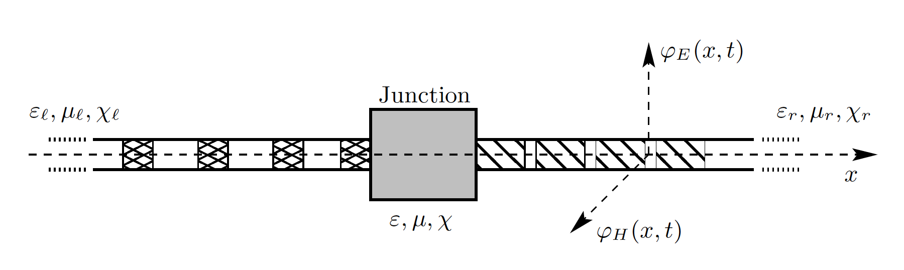 Figure 1
Peer Reviews
No public reviews on file for this paper yet. If you reviewed it on a platform where reviews are public (OpenReview, ICLR, NeurIPS, ICML), you can paste yours below so the community can read it here.
Videos
No videos yet. Explain this paper in a talk, walkthrough, or lecture? Add one.
Spectral and scattering theory of one-dimensional coupled photonic crystals
G. De Nittis1111Supported by the Chilean Fondecyt Grant 1190204., M. Moscolari2222Supported by the National Group of Mathematical Physics (GNFM-INdAM), S. Richard3333Supported by the grantTopological invariants through scattering theory and noncommutative geometry from Nagoya University, and by JSPS Grant-in-Aid for scientific research C no 18K03328, and on leave of absence from Univ. Lyon, Université Claude Bernard Lyon 1, CNRS UMR 5208, Institut Camille Jordan, 43 blvd. du 11 novembre 1918, F-69622 Villeurbanne cedex, France., R. Tiedra de Aldecoa1444Supported by the Chilean Fondecyt Grant 1170008.
Abstract
We study the spectral and scattering theory of light transmission in a system consisting of two asymptotically periodic waveguides, also known as one-dimensional photonic crystals, coupled by a junction. Using analyticity techniques and commutator methods in a two-Hilbert spaces setting, we determine the nature of the spectrum and prove the existence and completeness of the wave operators of the system.
**
- 1
Facultad de Matemáticas & Instituto de Física, Pontificia Universidad Católica de Chile,
Av. Vicuña Mackenna 4860, Santiago, Chile 2. 2
Fachbereich Mathematik, Eberhard-Karls-Universität, Auf der Morgenstelle 10, 72076 Tübingen, Germany 3. 3
Graduate school of mathematics, Nagoya University, Chikusa-ku,
Nagoya 464-8602, Japan 4. E-mails:* [email protected], [email protected], [email protected], [email protected]*
2010 Mathematics Subject Classification: 81Q10, 47A40, 47B47, 46N50, 35Q61.
Keywords: Spectral theory, scattering theory, Maxwell operators, commutator methods.
Contents
1 Introduction and main results
In this paper, we study the propagation of an electromagnetic field in an infinite one-dimensional waveguide. We assume that (i) the waveguide is parallel to the -axis of the Cartesian coordinate system; (ii) the electric field varies along the -axis and is constant on the planes perpendicular to the -axis, i.e., ; (iii) the magnetic field varies along the -axis and is constant on the planes perpendicular to the -axis, i.e., ; (iv) the waveguide is made of isotropic medium555The interaction between the electromagnetic field and the dielectric medium is characterised by the electric permittivity tensor and the magnetic permeability tensor . In an isotropic medium these tensors are multiple of the identity, and thus determined by two scalars.. Under these assumptions, one has and and the dynamical sourceless Maxwell equations [14] read as
[TABLE]
The scalar quantities and in (1.1) are the electric permittivity and magnetic permeability, respectively. They are strictly positive functions on describing the interaction of the waveguide with the electromagnetic field. One can also include in the model effects associated to bi-anisotropic media [21]. In our case, this is achieved by modifying the system (1.1) as follows :
[TABLE]
The (possibly complex-valued) function is called bi-anisotropic coupling term666In the general theory of bi-anisotropic media, is a tensor rather than a scalar. The system of equations (1.2) corresponds to a particular choice of the form of this tensor. For more details on the theory of bi-anisotropic media, we refer the interested reader to the monograph [21].. In the sequel, we will refer to the triple as the constitutive functions of the waveguide.
Let us first discuss the case of periodic waveguides, also known as one-dimensional photonic crystals, consisting in one-dimensional media with dielectric properties which vary periodically in space [15, 25, 44]. Mathematically, this translates into the fact that the functions and in (1.2) are periodic, all with the same period. This makes (1.2) into a coupled system of differential equations with periodic coefficients, and standard techniques like Bloch-Floquet theory (see e.g. [19]) can be used to study the propagation of solutions (or modes). One of the fundamental properties of periodic waveguides is the presence of a frequency spectrum made of bands and gaps. This implies that not all the modes can propagate along the medium, since the propagation of modes associated to frequencies inside a gap is forbidden by the “geometry” of the system. This phenomenon is similar to the one appearing in the theory of periodic Schrödinger operators, where one has electronic energy bands instead of frequency bands [28, Sec. XIII.16].
The study of the propagation of light in a periodic waveguide can be performed using Bloch-Floquet theory. The situation becomes more complicated when one wants to study the propagation of light through two periodic waveguides of different periods that are connected by a junction. Such a system is schematically represented in Figure 1. The asymptotic behaviour of the system on the left is characterised by the periodic constitutive functions , whereas the asymptotic behaviour of the system on the right is characterised by periodic constitutive functions . Namely, when and when , and similarly for the other two functions and (see Assumption 2.2 for a precise statement). The full system represented in Figure 1 can therefore be interpreted as a perturbation of a “free” system obtained by glueing together two purely periodic systems, one with periodicity of type on the left and the other with periodicity of type on the right. Accordingly, the analysis of the dynamics of the full system can be performed with the tools of spectral and scattering theories, leading us exactly to the main goal of this work : the spectral and scattering analysis of one-dimensional coupled photonic crystals.
Since quantum mechanics provides a rich toolbox for the study of problems associated to Schrödinger equations, we recast our equations of motion in a Schrödinger form to take advantage of these tools, in particular commutator methods which will be used extensively in this paper. Namely, with the notation w:=\big{(}\begin{smallmatrix}\varepsilon&\chi\\ \chi^{*}&\mu\end{smallmatrix}\big{)}^{-1} for the positive-definite matrix of weights associated to the constitutive functions , , (Maxwell weight for short), we rewrite the system of equations (1.2) in the matrix form
[TABLE]
so that it can be considered as a Schrödinger equation for the state in the Hilbert space . This observation is by no means new. Since the dawn of quantum mechanics, the founding fathers were well-aware that the Maxwell equations in vacuum are relativistically covariant equations for a massless spin-1 particle [39, pp. 151 & 198]. Moreover, similar Schrödinger formulations have already been employed in the literature to study the quantum scattering theory of electromagnetic waves and other classical waves in homogeneous media [5, 16, 27, 37, 41], and to study the propagation of light in periodic media [8, 9, 11, 20], among other things. However, to the best of our knowledge, the specific problem we want to tackle in the present work has never been considered in the literature.
The papers [27, 37, 41] deal with the scattering theory of three-dimensional electromagnetic waves in a homogeneous medium. In that setup, the constitutive tensors , , are asymptotically constant. In contrast, in our one-dimensional setup the constitutive functions , , are only assumed to be asymptotically periodic. This introduces a significant complication and novelty to the model, even though it has lower dimension than the three-dimensional models. Also, several works dealing with the scattering theory of electromagnetic waves are conducted under the simplifying assumption that (absence of bi-anisotropic effects), an assumption that we do not make in the present work. The papers [4, 40] deal with the transmission of the electric field and voltage along lines, also called one-dimensional Ohmic conductors. Mathematically, this problem is described by a system of differential equations similar to (1.2) or (1.3). However, in these papers, the constitutive quantities, namely the self-inductance and capacitance, are once again assumed to be asymptotically constant, in contrast with our less restrictive assumption of asymptotic periodicity. Finally, in the paper [43], almost no restrictions are imposed on the asymptotic behavior of the constitutive functions, but a stronger condition (invertibility) is imposed on the operator modelling the junction. Here, we do not assume that this operator is invertible or isometric, since we want to describe the scattering effects produced by the introduction of the junction itself, without imposing unnecessary conditions on the relation between the free dynamics without interface and the full dynamics in presence of the interface (see Remark 2.5 for more details). Also, even though the results of that paper hold in any space dimension, our results for one-dimensional photonic crystals are more detailed.
To conclude our overview of the literature, we point out that the dynamical equations describing our model are common to other physical systems. This is for instance the case of the equations describing the propagation of an Alfvén wave in a periodically stratified stationary plasma [2], the propagation of linearized water waves in a periodic bottom topography [7], or the propagation of harmonic acoustic waves in periodic waveguides [3]. In consequence, the results of our analysis here can be applied to all these models by reinterpreting in a appropriate way the necessary quantities.
Here is a description of our results. In Section 2.1, we introduce our assumption on the Maxwell weight (Assumption 2.2) and we define the full Hamiltonian in the Hilbert space describing the one-dimensional coupled photonic crystal. In Section 2.2, we define the free Hamiltonian in the Hilbert space associated to , and we define the operator modelling the junction depicted in Figure 1 (Definition 2.4). The operator is the direct sum of an Hamiltonian describing the periodic waveguide asymptotically on the left and an Hamiltonian describing the periodic waveguide asymptotically on the right. In Section 2.3, we use Bloch-Floquet theory to show that the asymptotic Hamiltonians and fiber analytically in the sense of Gérard and Nier [12] (Proposition 2.6). As a by-product, we prove that and do not possess flat bands, and thus have purely absolutely continuous spectra (Proposition 2.8). The analytic fibration of and provides also a natural definition for the set of thresholds in the spectrum of (Eqs. (2.5)-(2.6)). In section 3.1, we recall from [1, 33] the necessary abstract results on commutator methods for self-adjoint operators. In section 3.2, we construct for each compact interval a conjugate operator for the free Hamiltonian and use it to prove a limiting absorption principle for in (Theorem 3.3 and the discussion that follows). In Section 3.3, we use the fact that is a conjugate operator for and abstract results on the Mourre theory in a two-Hilbert spaces setting [32] to show that the operator is a conjugate operator for (Theorem 3.9). In Section 3.4, we use the operator to prove a limiting absorption principle for in , which implies in particular that in any compact interval the Hamiltonian has at most finitely many eigenvalues, each one of finite multiplicity, and no singular continuous spectrum (Theorem 3.15). Using Zhislin sequences (a particular type of Weyl sequences), we also show in Proposition 3.10 that and have the same essential spectrum. In Section 4.1, we recall abstract criteria for the existence and the completeness of wave operators in a two-Hilbert spaces setting. Finally, in Section 4.2, we use these abstract results in conjunction with the results of the previous sections to prove the existence and the completeness of wave operators for the pair (Theorem 4.6). We also give an explicit description of the initial sets of the wave operators in terms of the asymptotic velocity operators for the Hamiltonians and (Proposition 4.8 & Theorem 4.10).
2 Model
2.1 Full Hamiltonian
In this section, we introduce the full Hamiltonian that we will study. It is a one-dimensional Maxwell-like operator describing perturbations of an anisotropic periodic one-dimensional photonic crystal.
Throughout the paper, for any Hilbert space , we write for the scalar product on , for the norm on , for the set of bounded operators on , and for the set of compact operators on . We also use the notation (resp. ) for the set of bounded (resp. compact) operators from a Hilbert space to a Hilbert space .
Definition 2.1** (One-dimensional Maxwell-like operator).**
Let and take a Hermitian matrix-valued function w\in\mathop{\mathrm{L}^{\infty}}\nolimits\big{(}\mathbb{R},\mathscr{B}(\mathbb{C}^{2})\big{)} such that for a.e. . Let be the momentum operator in , that is, for each , with the first Sobolev space on . Let
[TABLE]
Then the Maxwell-like operator in is defined as
[TABLE]
The Maxwell weight that we consider converges at to periodic functions in the following sense :
Assumption 2.2** (Maxwell weight).**
There exist and hermitian matrix-valued functions w_{\ell},w_{\rm r}\in\mathop{\mathrm{L}^{\infty}}\nolimits\big{(}\mathbb{R},\mathscr{B}(\mathbb{C}^{2})\big{)} periodic of periods such that
[TABLE]
where the indexes and r stand for “left” and “right”, and .
Lemma 2.3**.**
Let Assumption 2.2 be satisfied.
- (a)
One has for a.e. the inequalities
[TABLE]
with introduced in Definition 2.1. 2. (b)
The sesquilinear form
[TABLE]
defines a new scalar product on , and we denote by the space equipped with . Moreover, the norm of and are equivalent, and the claim remains true if one replaces with or . 3. (c)
The operator with domain is self-adjoint in .
Proof.
Point (a) is a direct consequence of the assumptions on . Point (b) follows from the bounds valid for a.e. . Point (c) can be proved as in [10, Prop. 6.2]. ∎
2.2 Free Hamiltonian
We now define the free Hamiltonian associated to the operator . Due to the anisotropy of the Maxwell weight at , it is convenient to define left and right asymptotic operators
[TABLE]
with and as in Assumption 2.2. Lemma 2.3(c) implies that the operators and are self-adjoint in the Hilbert spaces and , with the same domain . Then we define the free Hamiltonian as the direct sum operator
[TABLE]
in the Hilbert space . Since the free Hamiltonian acts in the Hilbert space and the full Hamiltonian acts in the Hilbert space , we need to introduce an identification operator between the spaces and
Definition 2.4** (Junction operator).**
Let be such that
[TABLE]
Then is the bounded operator defined by
[TABLE]
with adjoint given by J^{*}\varphi=\big{(}w_{\ell}w^{-1}j_{\ell}\;\!\varphi,w_{\rm r}w^{-1}j_{\rm r}\;\!\varphi\big{)}.
Remark 2.5**.**
We call the junction operator because it models mathematically the junction depicted in Figure 1. Indeed, the Hamiltonian only describes the free dynamics of the system in the bulk asymptotically on the left and in the bulk asymptotically on the right. Since is the direct sum of the operators and , the interface effects between the left and the right parts of the system are not described by in any way. The role of the operator is thus to map the free bulk states of the system belonging to the direct sum Hilbert space onto a joined state belonging to the physical Hilbert space , where acts the full Hamiltonian describing the interface effects.
Given a state , the square norm can be interpreted as the total energy of the electromagnetic field . A direct computation shows that the total energy of a state obtained by joining bulk states and satisfies
[TABLE]
with and the total energies of the field on the left and the field on the right, and with
[TABLE]
the energy associated with the left and right external interfaces of the junction. In particular, one notices that there is no contribution to the energy associated to the central region of the junction. This physical observation shows as a by-product that the operator is neither invertible, nor isometric.
2.3 Fibering of the free Hamiltonian
In this section, we introduce a Bloch-Floquet (or Bloch-Floquet-Zak or Floquet-Gelfand) transform to take advantage of the periodicity of the operators and . For brevity, we use the symbol to denote either the index “” or the index “r”.
Let
[TABLE]
be the one-dimensional lattice of period with fundamental cell , and let
[TABLE]
be the reciprocal lattice of with fundamental cell . For each , we define the translation operator
[TABLE]
Using this operator, we can define the Bloch-Floquet transform of a -valued Schwartz function as
[TABLE]
One can verify that is -periodic in the variable ,
[TABLE]
and -pseudo-periodic in the variable ,
[TABLE]
Now, let be the Hilbert space obtained by equipping the set
[TABLE]
with the scalar product
[TABLE]
Since and are isomorphic, we shall use both representations. Next, let be the unitary representation of the dual lattice on given by
[TABLE]
and let be the Hilbert space obtained by equipping the set
[TABLE]
with the scalar product
[TABLE]
There is a natural isomorphism from to given by the restriction from to , and with inverse given by -equivariant continuation. However, using has various advantages and we shall stick to it in the sequel. Direct calculations show that the Bloch-Floquet transform extends to a unitary operator with inverse
[TABLE]
Furthermore, since commutes with the translation operators (), the operator is decomposable in the Bloch-Floquet representation. Namely, we have
[TABLE]
with
[TABLE]
and
[TABLE]
Here, the domain of satisfies
[TABLE]
with
[TABLE]
In the next proposition, we prove that the operator is analytically fibered in the sense of [12, Def. 2.2]. For this, we need to introduce the Bloch variety
[TABLE]
Proposition 2.6** (Fibering of the asymptotic Hamiltonians).**
Let
[TABLE]
- (a)
The set
[TABLE]
is open in and the map \mathcal{O}_{\star}\ni(\omega,z)\mapsto\big{(}\widehat{M_{\star}}(\omega)-z\big{)}^{-1}\in\mathscr{B}(\mathfrak{h}_{\star}) is analytic in the variables and . 2. (b)
For each , the operator has purely discrete spectrum. 3. (c)
If is equipped with the topology induced by , then the projection given by is proper.
In particular, the operator is analytically fibered in the sense of [12, Def. 2.2].
Proof.
(a) The operator is self-adjoint on , and for each we have that w_{\star}\big{(}\begin{smallmatrix}0&\omega\\ \omega&0\end{smallmatrix}\big{)}\in\mathscr{B}(\mathfrak{h}_{\star}). Hence, for each the operator is closed in and has domain , and for each the operator is self-adjoint on . In particular, we infer by functional calculus that
[TABLE]
Therefore, for each the set
[TABLE]
is non-empty, and then the argument in [17, Rem. IV.3.2] guarantees that is contained in the resolvent set of . Thus, for each the operator is closed in , has domain , and non-empty resolvent set, and for each the map is linear and therefore analytic. So, the collection is an analytic family of type (A) [28, p. 16], and thus also an analytic family in the sense of Kato [28, p. 14]. The claim is then a consequence of [28, Thm. XII.7].
(b) Since is an analytic family of type (A), the operators have compact resolvent (and thus purely discrete spectrum) either for all or for no [17, Thm. III.6.26 & VII.2.4]. Therefore, to prove the claim, it is sufficient to show that has compact resolvent. Now, we have
[TABLE]
where is a first order differential operator in with periodic boundary conditions, and thus with purely discrete spectrum that accumulates at . In consequence, each entry of the matrix operator
[TABLE]
is compact in , so that \big{(}\widehat{D}(0)+i\big{)}^{-1} is compact in . Since Lemma 2.3(a) implies that the norms on and are equivalent, we infer that \big{(}\widehat{D}(0)+i\big{)}^{-1} is also compact in . Finally, since
[TABLE]
with and bounded in , we obtain that \big{(}\widehat{M_{\star}}(0)+i\big{)}^{-1} is compact in .
(c) Let be endowed with the topology induced by . Point (a) implies that the set
[TABLE]
is open in . Therefore, the set is closed in and the inclusion is a closed map. Since the projection given by is also a closed map (because is compact, see [24, Ex. 7, p. 171]) and , we infer that is a closed map. Moreover, is continuous because it is the restriction to the subset of the continuous projection . In consequence, in order to prove that is proper it is sufficient to show that is compact in for each . But since
[TABLE]
this follows from compactness of and the closedness of in . ∎
Proposition 2.6 can be combined with the theorem of Rellich [17, Thm. VII.3.9] which, adapted to our notations, states :
Theorem 2.7** (Rellich).**
Let be a neighborhood of an interval and let be a self-adjoint analytic family of type (A), with each having compact resolvent. Then there is a sequence of scalar-valued functions and a sequence of vector-valued functions , all analytic on , such that for the are the repeated eigenvalues of and the form a complete orthonormal family of the associated eigenvectors of .
By applying this theorem to the family , we infer the existence of analytic eigenvalue functions and analytic orthonormal eigenvector functions . We call band the graph \{\big{(}k,\lambda_{\star,n}(k)\big{)}\mid k\in Y^{*}_{\star}\} of the eigenvalue function , so that the Bloch variety coincides with the countable union of the bands (see (2.3)). Since the derivative of exists and is analytic, it is natural to define the set of thresholds of the operator as
[TABLE]
and the set of thresholds of both and as
[TABLE]
Proposition 2.6(b), together with the analyticity of the functions , implies that the set is discrete, with only possible accumulation point at infinity. Furthermore, [28, Thm. XIII.85(e)] implies that the possible eigenvalues of are contained in . However, these eigenvalues should be generated by locally (hence globally) flat bands, and one can show their absence by adapting Thomas’ argument [38, Sec. II] to our setup :
Proposition 2.8** (Spectrum of the asymptotic Hamiltonians).**
The spectrum of is purely absolutely continuous. In particular,
[TABLE]
with the absolutely continuous spectrum of and the essential spectrum of .
Proof.
In view of [28, Thm. XIII.86], the claim follows once we prove the absence of flat bands for . For this purpose, we use the version of the Thomas’ argument as presented in [35, Sec. 1.3]. Accordingly, we first need to show that, for with large enough, the operator is invertible and satisfies
[TABLE]
Let us start with the operator
[TABLE]
acting on . Since the family of functions given by
[TABLE]
is an orthonormal basis of , and since and have equivalent norms, the family , with extended variable , is also a (non-orthogonal) basis for , and thus any can be expanded in as
[TABLE]
It follows that
[TABLE]
Thus, the operators are injective with closed range and satisfy in the relations
[TABLE]
In consequence , and the operators are invertible with
[TABLE]
It follows that is invertible too, with
[TABLE]
which implies (2.7).
Now, let us assume by contradiction that there exists such that is equal to a constant for all . Then using the analyticity properties of (Proposition 2.6) in conjunction with the analytic Fredholm alternative, one infers that is an eigenvalue of for all . Letting be the corresponding eigenfunction for , one obtains that for all . Choosing with and using the fact that is invertible, one thus obtains that
[TABLE]
which contradicts (2.7). ∎
Remark 2.9**.**
The absence of flat bands for the 3-dimensional Maxwell operator has been discussed in [35, Sec. 5]. However, the results of [35] do not cover the result of Proposition 2.8 since the weights considered in [35] are block-diagonal and smooth while in Proposition 2.8 the weights are positive-definite matrices. Neither diagonality, nor smoothness is assumed.
3 Mourre theory and spectral results
3.1 Commutators
In this section, we recall some definitions appearing in Mourre theory and provide a precise meaning to the commutators mentioned in the introduction. We refer to [1, 33] for more information and details.
Let be a self-adjoint operator in a Hilbert space with domain , and let . For any , we say that belongs to , with notation , if the map
[TABLE]
is strongly of class . In the case , one has if and only if the quadratic form
[TABLE]
is continuous for the norm topology induced by on . We denote by the bounded operator associated with the continuous extension of this form, or equivalently times the strong derivative of the function (3.1) at .
If is a self-adjoint operator in with domain and spectrum , we say that is of class if for some . In particular, is of class if and only if the quadratic form
[TABLE]
extends continuously to a bounded form defined by the operator . In such a case, the set is a core for and the quadratic form
[TABLE]
is continuous in the natural topology of (i.e. the topology of the graph-norm) [1, Thm. 6.2.10(b)]. This form then extends uniquely to a continuous quadratic form on which can be identified with a continuous operator from to the adjoint space . In addition, one has the identity
[TABLE]
and the following result is verified [1, Thm. 6.2.15] : If is of class for some and is a Schwartz function, then .
A regularity condition slightly stronger than being of class is defined as follows : is of class for some if is of class and if for some
[TABLE]
The condition is stronger than , which in turn is stronger than .
We now recall the definition of two useful functions introduced in [1, Sec. 7.2]. For this, we need the following conventions : if denotes the spectral projection-valued measure of , then we set E^{H}(\lambda;\varepsilon):=E^{H}\big{(}(\lambda-\varepsilon,\lambda+\varepsilon)\big{)} for any and , and if , then we write if is compact, and if there exists a compact operator such that . With these conventions, we define for of class the function by
[TABLE]
and we define the function by
[TABLE]
Note that the following equivalent definition of the function is often useful :
[TABLE]
One says that is conjugate to at a point if , and that is strictly conjugate to at if . It is shown in [1, Prop. 7.2.6] that the function is lower semicontinuous, that , and that if and only if . In particular, the set of points where is conjugate to ,
[TABLE]
is open in .
The main consequences of the existence of a conjugate operator for are given in the theorem below, which is a particular case of [33, Thm. 0.1 & 0.2]. For its statement, we use the notation for the point spectrum of , and we recall that if is an auxiliary Hilbert space, then an operator is locally -smooth on an open set if for each compact set there exists such that
[TABLE]
and is (globally) -smooth if (3.4) is satisfied with replaced by the identity .
Theorem 3.1** (Spectrum of ).**
Let be self-adjoint operators in a Hilbert space , let be an auxiliary Hilbert space, assume that is of class for some , and suppose there exist an open set , a number and an operator such that
[TABLE]
Then
- (a)
each operator which extends continuously to an element of \mathscr{B}\big{(}\mathcal{D}(\langle A\rangle^{s})^{*},\mathcal{G}\big{)} for some is locally -smooth on , 2. (b)
* has at most finitely many eigenvalues in , each one of finite multiplicity, and has no singular continuous spectrum in .*
3.2 Conjugate operator for the free Hamiltonian
With the definitions of Section 2.3 at hand, we can construct a conjugate operator for the operator . Our construction follows from the one given in [12, Sec. 3], but it is simpler because our base manifold is one-dimensional. Indeed, thanks to Theorem 2.7, it is sufficient to construct the conjugate operator band by band.
So, for each , let and be the bounded decomposable self-adjoint operators in defined by -equivariant continuation as in (2.2) and by the relations
[TABLE]
Set also and , with the operator of multiplication by the variable in
[TABLE]
Remark 3.2**.**
Since commutes with , the operator is self-adjoint in and essentially self-adjoint on . The definition and the domain of are independent of the specific weight appearing in the scalar product of . The insistence on the label is only motivated by a notational need that will result helpful in the next sections.
For any compact interval , we define the finite set \mathbb{N}(I):=\big{\{}n\in\mathbb{N}\mid\lambda_{\star,n}^{-1}(I)\neq\varnothing\big{\}}. Finally, we set
[TABLE]
Then we can define the symmetric operator in by
[TABLE]
Theorem 3.3** (Mourre estimate for ).**
Let be a compact interval. Then
- (a)
the operator is essentially self-adjoint on and on any other core for , with closure denoted by the same symbol, 2. (b)
the operator is of class , 3. (c)
there exists such that .
Proof.
(a) The claim is a consequence of Nelson’s criterion of self-adjointness [26, Thm. X.37] applied to the triple , where and . Indeed, the operator is essentially self-adjoint on since is essentially self-adjoint on . In addition, since is composed of the bounded operators and which are analytic in the variable and acts as in , a direct computation gives
[TABLE]
Similarly, a direct computation using the boundedness and the analyticity of and implies that
[TABLE]
In both inequalities, we used the fact that . As a consequence, is essentially self-adjoint on and on any other core for .
(b) The set
[TABLE]
is a core for . So, it follows from point (a) that is essentially self-adjoint on . Moreover, since is analytic in and satisfies the covariance relation (2.2), we obtain that for any . Since the same argument applies to the resolvent, we obtain that . Therefore, we have the inclusion for each , and a calculation using (3.2) gives
[TABLE]
Since \sum_{n\in\mathbb{N}(I)}\widehat{\Pi}_{\star,n}\;\!\big{|}\widehat{\lambda}^{\prime}_{\star,n}\big{|}^{2}\;\!\widehat{\Pi}_{\star,n}\in\mathscr{B}(\mathcal{H}_{\tau,\star}), it follows that is of class with
[TABLE]
Finally, since and for each , we infer from (3.8) and [1, Prop. 5.1.5] that is of class .
(c) Using point (b) and the definition of the operators , we obtain for all and that
[TABLE]
with c_{I}:=\min_{n\in\mathbb{N}(I)}\min_{\{k\in Y^{*}_{\star}\mid\lambda_{\star,n}(k)\in I\}}\big{|}\lambda^{\prime}_{n}(k)\big{|}^{2}. Thus, by using the definition of the scalar product in , we infer that
[TABLE]
which, together with the definition (3.3), implies the claim. ∎
Since the operator is essentially self-adjoint on and on any other core for , it follows by Theorem 3.3(a) that the inverse Bloch-Floquet transform of ,
[TABLE]
is essentially self-adjoint on and on any other core for . Therefore, the results (b) and (c) of Theorem 3.3 can be restated as follows : the operator is of class and there exists such that . Combining these results for and , one obtains a conjugate operator for the free Hamiltonian introduced in Section 2.2. Namely, for any compact interval , the operator
[TABLE]
satisfies the following properties :
- (a’)
the operator is essentially self-adjoint on and on any set with a core for , with closure denoted by the same symbol, 2. (b’)
the operator is of class , 3. (c’)
there exists such that .
Remark 3.4**.**
What precedes implies in particular that the free Hamiltonian has purely absolutely continuous spectrum except at the points of , where it may have eigenvalues. However, we already know from Proposition 2.8 that this does not occur. Therefore,
[TABLE]
3.3 Conjugate operator for the full Hamiltonian
In this section, we show that the operator is a conjugate operator for the full Hamiltonian introduced in Section 2.1. We start with the proof of the essential self-adjointness of in . We use the notation (see Remark 3.2) for the operator of multiplication by the variable in ,
[TABLE]
Proposition 3.5**.**
For each compact interval the operator is essentially self-adjoint on and on any other core for , with closure denoted by the same symbol.
Proof.
First, we observe that since with the operator is well-defined and symmetric on due to point (a’) above. Next, to prove the claim, we use Nelson’s criterion of essential self-adjointness [26, Thm. X.37] applied to the triple \big{(}A_{I},N,\mathscr{S}(\mathbb{R},\mathbb{C}^{2})\big{)} with .
For this, we note that is a core for and that the operators , , , and are bounded in . Moreover, we verify with direct calculations on that the operators and belong to (in ), and that their commutators and belong to (in ). Then a short computation using these properties gives the bound
[TABLE]
and a slightly longer computation using the same properties shows that
[TABLE]
Thus, the hypotheses of Nelson’s criterion are satisfied, and the claim follows. ∎
In order to prove that is a conjugate operator for , we need two preliminary lemmas. They involve the two-Hilbert spaces difference of resolvents of and
[TABLE]
Lemma 3.6**.**
For each , one has the inclusion .
Proof.
One has for
[TABLE]
Thus, an application of the standard result [34, Thm. 4.1] taking into account the properties of implies that the operator is compact. This proves the claim for the second term in (3.9).
For the first term in (3.9), we have the equalities
[TABLE]
with and matrix-valued functions vanishing at . Thus, the operator in the first term in (3.9) is also compact, which concludes the proof. ∎
Lemma 3.7**.**
For each and each compact interval , one has the inclusion
[TABLE]
Proof.
Since is essentially self-adjoint on , it is sufficient to show that
[TABLE]
Furthermore, we have , and each operator acts on as a sum , with bounded operators in mapping the set into . These facts, together with the compactness result of Lemma 3.6 and (3.9), imply that it is sufficient to show that
[TABLE]
and
[TABLE]
Now, if one takes Assumption 2.2 into account, the proof of these inclusions is similar to the proof of Lemma 3.6. We leave the details to the reader. ∎
Next, we will need the following theorem which is a direct consequence of Theorem 3.1 and Corollaries 3.7-3.8 of [32].
Theorem 3.8**.**
Let be self-adjoint operators in a Hilbert space , let be a self-adjoint operator in a Hilbert space , let , and let
[TABLE]
Suppose there exists a set such that is essentially self-adjoint on , with its self-adjoint extension. Finally, assume that
- (i)
* is of class ,* 2. (ii)
for each , one has , 3. (iii)
for each , one has , 4. (iv)
for each , one has .
Then is of class and . In particular, if is conjugate to at , then is conjugate to at .
We are now ready to prove a Mourre estimate for
Theorem 3.9** (Mourre estimate for ).**
Let be a compact interval. Then is of class , and
[TABLE]
Proof.
Theorem 3.3 and its restatement at the end of Section 3.2 give us the estimate
[TABLE]
In addition, the equality \widetilde{\varrho}_{M_{0}}^{A_{0,I}}=\min\big{\{}\widetilde{\varrho}_{M_{\ell}}^{A_{\ell,I}},\widetilde{\varrho}_{M_{\rm r}}^{A_{{\rm r},I}}\big{\}} is a consequence of the definition of as a direct sum of and (see [1, Prop. 8.3.5]).
So, it only remains to show the inequality to prove the claim. For this, we apply Theorem 3.8 with , and , starting with the verification of its assumptions (i)-(iv) : the assumptions (i), (ii) and (iii) of Theorem 3.8 follow from point (b’) above, Lemma 3.6, and Lemma 3.7, respectively. Furthermore, the assumption (iv) of Theorem 3.8 follows from the fact that for any we have the inclusion
[TABLE]
since
[TABLE]
is a matrix-valued function vanishing at . These facts, together with Proposition 3.5 and the inclusion , imply that all the assumptions of Theorem 3.8 are satisfied. We thus obtain that , as desired. ∎
3.4 Spectral properties of the full Hamiltonian
In this section, we determine the spectral properties of the full Hamiltonian . We start by proving that has the same essential spectrum as the free Hamiltonian
Proposition 3.10**.**
One has
[TABLE]
To prove Proposition 3.10, we first need two preliminary lemmas. In the first lemma, we use the notation for the characteristic function of a Borel set .
Lemma 3.11**.**
- (a)
The operator is locally compact in , that is, for each bounded Borel set . 2. (b)
Let \zeta\in C^{\infty}_{\rm c}\big{(}\mathbb{R},[0,\infty)\big{)} satisfy for and for , and set for all and . Then
[TABLE]
Moreover, the results of (a) and (b) also hold true for the operators and in the Hilbert space .
Proof.
(a) A direct computation shows that
[TABLE]
which implies that is compact in since every entry of the matrix is compact in (see [34, Thm. 4.1]). Given that and have equivalent norms by Lemma 2.3(b), it follows that is also compact in . Finally, the resolvent identity (similar to (2.4))
[TABLE]
shows that is the sum of two compact operators in , and hence compact in . The same argument also shows that the operators are locally compact in , and thus that is locally compact in .
(b) Let . Then a direct computation taking into account the inclusion gives
[TABLE]
In consequence, we obtain that \big{\|}[M,\zeta_{n}(Q)](M-i)^{-1}\big{\|}_{\mathscr{B}(\mathcal{H}_{w})}\leq{\rm Const.}\;\!n^{-1} which proves the claim. As before, the same argument also applies to the operators in , and thus to the operator in . ∎
Lemma 3.11 is needed to prove that the essential spectra of and can be characterised in terms of Zhislin sequences (see [13, Def. 10.4]). Zhislin sequences are particular types of Weyl sequences supported at infinity as in the following lemma :
Lemma 3.12** (Zhislin sequences).**
Let . Then if and only if there exists a sequence , called Zhislin sequence, such that :
- (a)
* for all ,* 2. (b)
for each , one has if , 3. (c)
.
Similarly, if and only if there exists a sequence which meets the properties (a), (b), (c) relative to the operator .
Proof.
In view of Lemma 3.11, the claim can be proved by repeating step by step the arguments in the proof of [13, Thm. 10.6]. ∎
We are now ready to complete the description of the essential spectrum of
Proof of Proposition 3.10.
Take , let be an associated Zhislin sequence, and define for each
[TABLE]
Then one has \big{\|}\phi^{0}_{m}\big{\|}_{\mathcal{H}_{0}}=1 for all and if . Furthermore, using successively the facts that , that , and that , one obtains that
[TABLE]
which implies that due to Assumption 2.2.
Now, consider the inequalities
[TABLE]
From the property (c) of Zhislin sequences, the boundedness of , and the equivalence of the norms of and , one gets that
[TABLE]
Moreover, one has [M,j_{\star}]\;\!\phi_{m}=-iwj_{\star}^{\prime}\big{(}\begin{smallmatrix}0&1\\ 1&0\end{smallmatrix}\big{)}\phi_{m}, with supported in . This implies that . For the same reason, one has , with the latter vector supported in if and in if . This, together with Assumption 2.2, implies that
[TABLE]
The last inequality, along with the equality (which follows from the property (c) of Zhislin sequences), gives
[TABLE]
Putting all the pieces together, we obtain that \lim_{m\to\infty}\big{\|}(M_{0}-\lambda)\phi^{0}_{m}\big{\|}_{\mathcal{H}_{0}}=0. This concludes the proof that is a Zhislin sequence for the operator and the point , and thus that .
For the opposite inclusion, take a Zhislin sequence for the operator and the point , and assume that (if , then and the same proof applies if one replaces “right” with “left”). By extracting the nonzero right components from and normalising, we can form a new Zhislin sequence for with a Zhislin sequence for . Then we can construct as follows a new Zhislin sequence for with vectors supported in : Let satisfy for and for , set for all and , and choose such that \big{\|}\chi_{[-n_{m}^{\rm r},\infty)}(Q_{\rm r})\phi_{m}^{\rm r}\big{\|}_{\mathcal{H}_{w_{\rm r}}}\in(1-1/m,1]. Next, define for each
[TABLE]
with d_{m}:=\big{\|}\zeta^{\rm r}_{m}(Q_{\rm r})T_{k_{m}^{\rm r}p_{\rm r}}\phi_{m}^{\rm r}\big{\|}^{-1}_{\mathcal{H}_{w_{\rm r}}}, such that , and the operator of translation by . One verifies easily that and that has support in . Furthermore, since the operators and commute, one also has
[TABLE]
which implies that \lim_{m\to\infty}\big{\|}(M_{\rm r}-\lambda)\widetilde{\phi}_{m}^{\rm r}\big{\|}_{\mathcal{H}_{w_{\rm r}}}=0. Thus, is a new Zhislin sequence for with supported in .
Now, define for each
[TABLE]
Then one has for all and if . Furthermore, using that
[TABLE]
one obtains that
[TABLE]
which implies that due to Assumption 2.2. Now, consider the inequality
[TABLE]
From the property (c) of Zhislin sequences and the equivalence of the norms of and , one gets that
[TABLE]
Moreover, since is supported in , one infers again from Assumption 2.2 that
[TABLE]
The last inequality, along with the equality \lim_{m\to\infty}\big{\|}M_{\rm r}\widetilde{\phi}_{m}^{\rm r}\big{\|}_{\mathcal{H}_{w_{\rm r}}}=|\lambda|, gives
[TABLE]
Putting all the pieces together, we obtain that \lim_{m\to\infty}\big{\|}(M-\lambda)\phi_{m}\big{\|}_{\mathcal{H}_{w}}=0. This concludes the proof that is a Zhislin sequence for the operator and the point , and thus that . In consequence, we obtained that , which completes the proof in view of Remark 3.4. ∎
In order to determine more precise spectral properties of , we now prove that for each compact interval the Hamiltonian is of class for some , which is a regularity condition slightly stronger than the condition of class already established in Theorem 3.9. We start by giving a convenient formula for the commutator , , in the form sense on
[TABLE]
with
[TABLE]
and
[TABLE]
As already shown in the previous section, all the terms in extend to bounded operators, and we keep the same notation for these extensions.
In order to show that , it is enough to prove that and to check that
[TABLE]
Since the first proof reduces to computations similar to the ones presented in the previous section, we shall concentrate on the proof of (3.11). First of all, algebraic manipulations as presented in [1, pp. 325-326] or [30, Sec. 4.3] show that for all
[TABLE]
Furthermore, if we set and , we obtain that
[TABLE]
with due to (3.7). Thus, since \big{\|}A_{t}+i(tA_{I}+i)^{-1}A_{I}\;\!\langle Q\rangle^{-1}\big{\|}_{\mathscr{B}(\mathcal{H}_{w})} is bounded by a constant independent of , it is sufficient to prove that
[TABLE]
and to prove this estimate it is sufficient to show that the operators and defined in the form sense on extend continuously to elements of . Finally, some lengthy but straightforward computations show that these two last conditions are implied by the following two lemmas :
Lemma 3.13**.**
* is of class for each and .*
Proof.
One can verify directly that the unitary group generated by the operator leaves the domain invariant and that the commutator defined in the form sense on extends continuously to a bounded operator. Since the set is a core for , these properties together with [1, Thm. 6.3.4(a)] imply the claim. ∎
Lemma 3.14**.**
One has for each and each compact interval .
Proof.
By using the commutator expansions [1, Thm. 5.5.3] and (3.7), one gets the following equalities in form sense on
[TABLE]
with and with each commutator in the last equality extending continuously to a bounded operator. Since is integrable, the last two terms give bounded contributions. Furthermore, the first two terms can be rewritten as
[TABLE]
with
[TABLE]
But, since for each , and since is a Schwartz function, one infers from [1, Thm. 5.5.3] that the operator f\big{(}[Q_{\star},\Pi_{\star,n}\widecheck{\lambda}^{\prime}_{\star,n}\Pi_{\star,n}]\big{)} is regularising in the Besov scale associated to the operator . This implies in particular that the operators f\big{(}[Q_{\star},\Pi_{\star,n}\widecheck{\lambda}^{\prime}_{\star,n}\Pi_{\star,n}]\big{)}Q_{\star} and Q_{\star}f\big{(}[Q_{\star},\Pi_{\star,n}\widecheck{\lambda}^{\prime}_{\star,n}\Pi_{\star,n}]\big{)} extend continuously to bounded operators, as desired. ∎
We can now give in the next theorem a description of the structure of the spectrum of the full Hamiltonian . The next theorem also shows that the set can be interpreted as the set of thresholds in the spectrum of
Theorem 3.15**.**
In any compact interval , the operator has at most finitely many eigenvalues, each one of finite multiplicity, and no singular continuous spectrum.
Proof.
The computations at the beginning of this section together with Lemmas 3.13 & 3.14 imply that is of class for some , and Theorem 3.9 implies that the condition (3.5) of Theorem 3.1 is satisfied on . So, one can apply Theorem 3.1(b) to conclude. ∎
Remark 3.16**.**
As a final remark about the spectral properties of the operator , let us mention that the techniques used in this work do not provide any further information about the existence of eigenvalues at thresholds or embedded in the continuous spectrum. For additive perturbations, powerful techniques have been developed over the last decades, and these methods can be applied to several Schrödinger-type operators. On the other hand, for multiplicative perturbations, abstract methods have not been developed so far. To the best of our knowledge, there exist only a few results about embedded eigenvalues in the case of quantum walks with multiplicative perturbations as for example in [18, 22, 23], or more abstractly in [6]. For photonic crystals, especially in the presence of bi-anisotropic media, eigenvalues at thresholds or embedded in the continuous spectrum certainly deserve an independent study and this could be the subject of future investigations.
4 Scattering theory
4.1 Scattering theory in a two-Hilbert spaces setting
We discuss in this section the existence and the completeness, under smooth perturbations, of the local wave operators for self-adjoint operators in a two-Hilbert spaces setting. Namely, given two self-adjoint operators in Hilbert spaces with spectral measures , an identification operator , and an open set , we recall criteria for the existence and the completeness of the strong limits
[TABLE]
under the assumption that the two-Hilbert spaces difference of resolvents
[TABLE]
factorises as a product of a locally -smooth operator on and a locally -smooth operator on .
We start by recalling some facts related to the notion of -completeness. Let be the subsets of defined by
[TABLE]
Then it is clear that are closed subspaces of and that , and it is shown in [42, Sec. 3.2] that is reduced by and that
[TABLE]
In particular, one has the inclusion
[TABLE]
which motivates the following definition :
Definition 4.1** (-completeness).**
Assume that the local wave operators exist. Then are -complete on if
[TABLE]
Remark 4.2**.**
In the particular case and , the -completeness on reduces to the completeness of the local wave operators on in the usual sense. Namely, \overline{\mathop{\mathrm{Ran}}\nolimits\big{(}W_{\pm}(H,H_{0},1_{\mathcal{H}},I)\big{)}}=E^{H}(I)\mathcal{H}, and the operators are unitary from to .
The following criterion for -completeness has been established in [42, Thm. 3.2.4] :
Lemma 4.3**.**
If the local wave operators and exist, then are -complete on .
For the next theorem, we recall that the spectral support of a vector with respect to is the smallest closed set such that .
Theorem 4.4**.**
Let be self-adjoint operators in Hilbert spaces with spectral measures , , an open set, and an auxiliary Hilbert space. For each , assume there exist locally -smooth on and locally -smooth such that
[TABLE]
Then the local wave operators
[TABLE]
exist, are -complete on , and satisfy the relations
[TABLE]
for each bounded Borel function .
Proof.
We adapt the proof of [1, Thm. 7.1.4] to the two-Hilbert spaces setting. The existence of the limits (4.1) is a direct consequence of the following claims : for each with compact, and for each such that on a neighbourhood of , we have that
[TABLE]
To prove the first claim in (4.2), take and , and observe that the operators satisfy for and
[TABLE]
with and the constant appearing in the definition (3.4) of a locally -smooth operator. Since the set is dense in and is locally -smooth on , it follows that \big{\|}\big{(}W(t)-W(s)\big{)}(H_{0}-z)^{-1}\varphi_{0}\big{\|}_{\mathcal{H}}\to 0 as or . Applying this result with replaced by we infer that
[TABLE]
as or , which proves the first claim in (4.2).
To prove the second claim in (4.2), we take such that on and . Then we have and
[TABLE]
and thus the second claim in (4.2) follows from
[TABLE]
Since the vector space generated by the functions , , is dense in , it is sufficient to show that
[TABLE]
Now, we have for every
[TABLE]
Therefore, it is enough to prove that \big{\|}T_{0}(z)\mathop{\mathrm{e}}\nolimits^{-itH_{0}}\varphi_{0}\big{\|}_{\mathcal{G}}\to 0 as . But since and its derivative are square integrable in , this follows from a standard Sobolev embedding argument. So, the existence of the limits (4.1) has been established. Similar arguments, using the relation
[TABLE]
instead of
[TABLE]
show that exists too. This, together with standard arguments in scattering theory, implies the claims that follow (4.1). ∎
As a consequence of Theorem 3.1(a) & Theorem 4.4, we obtain the following criterion for the existence and completeness of the local wave operators :
Corollary 4.5**.**
Let be self-adjoint operators in Hilbert spaces with spectral measures and self-adjoint operators in . Assume that are of class for some . Let
[TABLE]
, an auxiliary Hilbert space, and for each suppose there exist and with
[TABLE]
and such that extends continuously to an element of \mathscr{B}\big{(}\mathcal{D}(\langle A_{0}\rangle^{s})^{*},\mathcal{G}\big{)} and extends continuously to an element of \mathscr{B}\big{(}\mathcal{D}(\langle A\rangle^{s})^{*},\mathcal{G}\big{)} for some . Then the local wave operators
[TABLE]
exist, are -complete on , and satisfy the relations
[TABLE]
for each bounded Borel function .
4.2 Scattering theory for one-dimensional coupled photonic crystals
In the case of the pair , we obtain the following result on the existence and completeness of the wave operators; we use the notation for the orthogonal projection on the absolutely continuous subspace of
Theorem 4.6**.**
Let . Then the local wave operators
[TABLE]
exist and satisfy \overline{\mathop{\mathrm{Ran}}\nolimits\big{(}W_{\pm}(M,M_{0},J,I_{\rm max})\big{)}}=E_{\rm ac}^{M}\;\!\mathcal{H}_{w}. In addition, the relations
[TABLE]
and
[TABLE]
hold for each bounded Borel function .
Proof.
All the claims except the equality \overline{\mathop{\mathrm{Ran}}\nolimits\big{(}W_{\pm}(M,M_{0},J,I_{\rm max})\big{)}}=E_{\rm ac}^{M}\;\!\mathcal{H}_{w} follow from Corollary 4.5 whose assumptions are verified below.
Let be a compact interval. Then we know from Section 3.2 that is of class and from Section 3.4 that is of class for some . Moreover, Theorems 3.3 & 3.9 imply that
[TABLE]
Therefore, in order to apply Corollary 4.5, it is sufficient to prove that for any the operator
[TABLE]
factorises as a product of two locally smooth operators as in (4.3). For that purpose, we set with , we define
[TABLE]
and we consider the sesquilinear form
[TABLE]
Our first goal is to show that this sesquilinear form is continuous for the topology of . However, since the necessary computations are similar to the ones presented in Sections 3.3-3.4, we only sketch them. We know from (3.9) that
[TABLE]
So, we have to establish the continuity of the sesquilinear forms
[TABLE]
and
[TABLE]
For the first one, we know from (3.10) that
[TABLE]
By inserting this expression into (4.5), by taking the -property of and into account, and by observing that the operators , and defined on extend continuously to elements of , one obtains that the sesquilinear forms defined by the first two terms in (4.7) are continuous for the topology of . The sesquilinear form defined by the third term in (4.7) and the sesquilinear form (4.6) can be treated simultaneously. Indeed, the factor can be computed explicitly and contains a factor which has compact support. Therefore, since , a few more commutator computations show that the two remaining sesquilinear forms are continuous for the topology of .
In consequence, the sesquilinear form (4.4) is continuous for the topology of , and thus corresponds to a bounded operator . Therefore, if we set
[TABLE]
we obtain that . On another hand, we know from computations presented in Section 3.4 that
[TABLE]
and
[TABLE]
So, we have the inclusions
[TABLE]
and thus all the assumptions of Corollary 4.5 are verified.
Hence it only remains to show that \overline{\mathop{\mathrm{Ran}}\nolimits\big{(}W_{\pm}(M,M_{0},J,I_{\rm max})\big{)}}=E_{\rm ac}^{M}\;\!\mathcal{H}_{w}. For that purpose, we first recall from the proof of Theorem 3.9 that . Then since has purely absolutely continuous spectrum in one infers from the RAGE theorem that
[TABLE]
and consequently that . By using the -completeness on of the local wave operators and that has purely absolutely continuous spectrum in , we thus obtain
[TABLE]
By putting together these results for different intervals and by using Proposition 3.10, we thus get that
[TABLE]
which concludes the proof. ∎
Remark 4.7**.**
Let be a compact interval and let . Then we have
[TABLE]
with
[TABLE]
and given by
[TABLE]
That is, the operators act as the sum of the local wave operators
[TABLE]
In order to get a better understanding of the initial sets of the partial isometries some preliminary considerations on the asymptotic velocity operators for and are necessary. First, we define for each and the spaces
[TABLE]
and note that decomposes into the internal direct sum and that the operator is reduced by this decomposition, namely, . Next, we introduce the self-adjoint operator in
[TABLE]
Then it is natural to define the asymptotic velocity operator for in as
[TABLE]
and the asymptotic velocity operator for in as the direct sum
[TABLE]
Additionally, we define the family of self-adjoint operators in
[TABLE]
and the corresponding family of self-adjoint operators in
[TABLE]
Our next result is inspired by the result of [36, Thm. 4.1] in the setup of quantum walks. In the proof, we use the linear span of elements of
[TABLE]
Proposition 4.8**.**
For each and , we have
[TABLE]
Proof.
For each , we have the inclusion \mathscr{U}_{\star}^{-1}\mathcal{H}_{\star,\tau}^{\rm fin}\subset\big{\{}\mathcal{D}(V_{\star})\cap\mathcal{D}\big{(}Q_{\star}(t)\big{)}\big{\}}. Furthermore, if , then we have
[TABLE]
As a consequence, the following equality holds for all and
[TABLE]
Since \big{\|}\big{(}\frac{Q_{\star}(t)}{t}-z\big{)}^{-1}\big{\|}_{\mathscr{B}(\mathcal{H}_{w_{\star}})}\leq|\mathop{\mathrm{Im}}\nolimits(z)|^{-1} and \big{\|}(V_{\star}-z)^{-1}\big{\|}_{\mathscr{B}(\mathcal{H}_{w_{\star}})}\leq|\mathop{\mathrm{Im}}\nolimits(z)|^{-1}, and since is dense in , it follows that it is sufficient to prove that
[TABLE]
Now, a direct calculation using the Bloch-Floquet transform gives for with
[TABLE]
where in the last equation we have used that acts as in . Since , the summation over is finite, and since the map Y^{*}_{\star}\ni k\mapsto\big{(}\widehat{Q_{\star}}\widehat{\Pi}_{\star,n}u\big{)}(k)\in\mathfrak{h}_{\star} is bounded, one deduces that
[TABLE]
which implies the claim. ∎
In the next proposition, we determine the initial sets of the isometries defined in (4.8). In the statement, we use the fact that the operators and strongly commute. We also use the notations and for the characteristic functions of the intervals and , respectively.
Proposition 4.9**.**
- (a)
Let be a compact interval, then the operators are partial isometries with initial sets . 2. (b)
Let be a compact interval, then the operators are partial isometries with initial sets .
Before the proof, let us observe that if is a compact interval, then we have the equalities
[TABLE]
due to the definition of the set .
Proof.
Our proof is inspired by the proof of [31, Prop. 3.4]. We first show the claim for . So, let . If , then \varphi_{\ell}\in\ker\big{(}W_{+}(M,M_{\ell},J_{\ell},I)\big{)}. Thus, we can assume that . Next, let us show that if then again \varphi_{\ell}\in\ker\big{(}W_{+}(M,M_{\ell},J_{\ell},I)\big{)}. For this, assume that for some . Then it follows from (4.8)-(4.9) that
[TABLE]
Now, let satisfy if and if . Then one has for each the inequality
[TABLE]
Furthermore, since , one infers from Proposition 4.8 and from a standard result on strong resolvent convergence [29, Thm. VIII.20(b)] that
[TABLE]
Putting together what precedes, one obtains that \varphi_{\ell}=\chi_{[\varepsilon,\infty)}(V_{\ell})\varphi_{\ell}\in\ker\big{(}W_{+}(M,M_{\ell},J_{\ell},I)\big{)}, and then a density argument taking into account the second equation in (4.10) implies that
[TABLE]
To show that is an isometry on , take with for some , and let satisfy if and if . Then using successively the identity , the unitarity of in and of in , the definition (4.9) of , the definition of , and the fact that , one gets
[TABLE]
For the first term one has
[TABLE]
while the second term also vanishes by an application of the RAGE theorem. It follows that is isometric on , and then a density argument taking into account the first equation in (4.10) implies that is isometric on .
A similar proof works for the claims about and . The functions and have to be adapted and the possible negative sign of the variable has to be taken into account, otherwise the argument can be copied mutatis mutandis. ∎
By collecting the results of Theorem 4.6, Remark 4.7, Proposition 4.9, and by using the fact that and have purely absolutely continuous spectrum, one finally obtains a description of the initial sets of the local wave operators
Theorem 4.10**.**
Let and (). Then the local wave operators are partial isometries with initial sets
[TABLE]
Remark 4.11**.**
One has because is discrete and (see Proposition 2.8 and the paragraph that precedes). Therefore, the spectral projections in the statement of Theorem 4.10 can be removed if desired.
The reference list from the paper itself. Each links out to its DOI / PubMed record.
- 1[1] W. O. Amrein, A. Boutet de Monvel, and V. Georgescu, C 0 subscript 𝐶 0 C_{0} -groups, commutator methods and spectral theory of N 𝑁 N -body Hamiltonians , volume 135 of Progress in Mathematics , Birkhäuser Verlag, Basel, 1996.
- 2[2] R. Alicki, Dirac equations for MHD waves: Hamiltonian spectra and supersymmetry, J. Phys. A: Math. Gen. 25: 6075–6085, 1992.
- 3[3] C. E. Bradley, Time harmonic acoustic Bloch wave propagation in periodic waveguides. Part I. Theory, J. Acoust. Soc. Am. 96(3): 1844–1853, 1994.
- 4[4] G. L. Brown, The Inverse Reflection Problem for Electric Waves on Non-Uniform Transmission Lines , Thesis, Univ. of Wisconsin 1965.
- 5[5] M. S. Birman and M. Z. Solomyak, L 2 subscript 𝐿 2 L_{2} -Theory of the Maxwell operator in arbitrary domains, Uspekhi Mat. Nauk 42(6): 61–76, 1987.
- 6[6] O. Bourget, On embedded bound states of unitary operators and their regularity , Bulletin des Sciences Mathématiques 137(1): 1–29, 2013.
- 7[7] W. Craig, M. Gazeau, C. Lacave, and C. Sulem, Bloch Theory and Spectral Gaps for Linearized Water Waves, SIAM J. Math. Anal. 50(5): 5477–5501, 2018.
- 8[8] G. De Nittis and M. Lein, Effective Light Dynamics in Perturbed Photonic Crystals, Comm. Math. Phys. 332: 221–260, 2014.