This paper presents a method to reconstruct a smooth manifold from a uniform sample by constructing a function whose zero set approximates the manifold with guarantees on accuracy and local properties.
Contribution
It introduces a novel function construction from samples that accurately approximates the manifold and provides local support and projection methods for reconstruction.
Findings
01
Zero set of the constructed function is homeomorphic to the manifold.
02
Hausdorff distance between the approximation and the manifold is $O(m^{5/2}\varepsilon^{2})$.
03
Projection operator converges to the manifold approximation.
Abstract
Let M⊂Rd be a compact, smooth and boundaryless manifold with dimension m and unit reach. We show how to construct a function φ:Rd→Rd−m from a uniform (ε,κ)-sample P of M that offers several guarantees. Let Zφ denote the zero set of φ. Let M denote the set of points at distance ε or less from M. There exists ε0∈(0,1) that decreases as d increases such that if ε≤ε0, the following guarantees hold. First, Zφ∩M is a faithful approximation of M in the sense that Zφ∩M is homeomorphic to M, the Hausdorff distance between Zφ∩M and M is O(m5/2ε2), and the normal spaces at…
No public reviews on file for this paper yet. If you reviewed it on a platform where reviews are public (OpenReview, ICLR, NeurIPS, ICML), you can paste yours below so the community can read it here.
Videos
No videos yet. Explain this paper in a talk, walkthrough, or lecture? Add one.
Taxonomy
TopicsAdvanced Mathematical Modeling in Engineering · Numerical methods in inverse problems · Advanced Numerical Analysis Techniques
Full text
Implicit Manifold Reconstruction††thanks: A preliminary version
appears in Proceedings of the 25th Annual ACM-SIAM Symposium on Discrete Algorithms, 2014, 161–173.
Siu-Wing Cheng111Supported by Research Grants Council, Hong Kong, China (project no. 612109). Department of Computer Science and Engineering, HKUST, Hong Kong.
Man-Kwun Chiu222Supported by JST ERATO Grant Number JPMJER1201, Japan and ERC StG 757609. Institut für Informatik, Freie Universität Berlin, Berlin, Germany.
Let M⊂Rd be a compact, smooth and boundaryless manifold with dimension m
and unit reach. We show how to construct a function φ:Rd→Rd−m from a uniform (ε,κ)-sample P of M
that offers several guarantees. Let Zφ denote the zero set of
φ. Let M denote the set of points at distance
ε or less from M. There exists ε0∈(0,1) that decreases as d increases such that if ε≤ε0, the following guarantees hold. First, Zφ∩M is a faithful approximation of M in the sense that Zφ∩M is
homeomorphic to M, the Hausdorff distance between Zφ∩M and M is O(m5/2ε2), and the normal spaces at nearby
points in Zφ∩M and M make an angle
O(m2κε). Second, φ has local support; in particular,
the value of φ at a point is affected only by sample points in P that
lie within a distance of O(mε). Third, we give a projection operator that
only uses sample points in P at distance O(mε) from the initial point.
The projection operator maps any initial point near P onto Zφ∩M in the limit by repeated applications.
1 Introduction
Sensory devices and numerical experiments may generate numerous data points in
Rd for some large d due to the large number of attributes of the data
that are being monitored. It is often believed that the data points are
governed by some hidden processes with fewer controlling parameters, and
therefore, the data points may lie in some m-dimensional manifold M
for some m≪d. This motivates the study of manifold reconstruction.
In computational geometry, there are several known results that offer provably
faithful reconstructions in the sense that the reconstruction is topologically
equivalent to M, the Hausdorff distance between the reconstruction and
M decreases as the sampling density increases, and the angular error
between the tangent spaces at nearby points in the reconstruction and M
decreases as the sampling density increases. These include the weighted cocone
complex by Cheng, Dey and Ramos [13], the weighted witness complex by
Boissonnat, Guibas and Oudot [9], and the tangential Delaunay complex by
Boissonnat and Ghosh [8]. These reconstructions are m-dimensional
simplicial complexes with the given sample points as vertices.
The corresponding reconstruction algorithms have to deal with the challenging
issue of “sliver removal” in high dimensions.
Solutions of partial differential equations on manifolds are required in quite
a few areas such as biology [33], image processing [41, 43],
weathering [18], and fluid dynamics [36, 37]. The
underlying manifold is often specified by a point cloud. It has been reported [31] that local reconstructions of a manifold in the form of zero level sets of local functions are preferred for solving partial differential equations on the manifold.
Several numerical methods for solving partial differential equations on level sets have been developed [5, 22, 31, 38].
In this paper, we propose an implicit reconstruction for manifolds with
arbitrary codimension in Rd. Let M be a compact, smooth, and
boundaryless manifold with unit reach.
Let P be a uniform
(ε,κ)-sample of M, that is, every point in M is at distance
ε or less from some point in P and the number of sample points inside any d-ball of radius ε is at most some constant κ. We assume that the following
information is specified in the input: (i) the manifold dimension m, (ii) a
neighborhood radiusγ=4ε, and (iii) approximate tangent spaces at points in P
such that the true tangent space at each point in P makes an angle at most mγ with the given approximate tangent space at that point. There are many
algorithms for estimating the manifold dimension
(e.g. [12, 14, 25, 30, 40]). When the sample points satisfy some local
uniformity condition (e.g., a constant upper bound on the number of sample
points inside any ball of radius ε centered in M), the neighborhood
radius γ can be set by measuring the maximum distance from a sample
point to its kth nearest neighbor for some appropriate k. If the sample
points are drawn from an independent and identical distribution on M, a
recently proposed reach estimator can be used to set γ [3].
There are many algorithms for estimating tangent spaces
(e.g. [4, 11, 23, 32, 39]), which give an O(ε) angular error.
We use the conditions of γ=4ε and angular error at most mγ in order to keep the number of unknown parameters small. One may worry about satisfying these two conditions simultaneously, but it is not a concern as we explain below. Suppose that the estimation algorithms return an angular error bound of cε for some known constant c≥1 and a value ℓ such that ε≤ℓ=O(ε). We can set γ=max{4ℓ,cℓ}. Then, the angular error is at most cε≤cℓ≤mγ. Moreover, letting c′=max{εℓ,4εcℓ}, the input sample can be viewed as a uniform (ε′,κ′)-sample, where ε′=c′ε=γ/4 and κ′=(2c′+1)dκ, because a packing argument shows that if any d-ball of radius ε contains at most κ sample points, then any d-ball of radius c′ε contains at most (2c′+1)dκ sample points.
Our main result is a formula for a function φ:Rd→Rd−m using the (ε,κ)-sample P and the neighborhood radius γ such that
the zero set of φ near M forms a reconstruction of M. Let Zφ denote the zero set of φ. Let M denote the set of points at distance ε or less from M. We prove that there exists ε0∈(0,1) that decreases as d increases such that if ε≤ε0, the following guarantees hold. First, Zφ∩M is a faithful approximation of M in the sense that
Zφ∩M is homeomorphic to M, the Hausdorff
distance between Zφ∩M and M is
O(m5/2γ2)=O(m5/2ε2), and the normal spaces at nearby points in Zφ∩M and M make an angle O(m2κγ)=O(m2κε). Second,
φ has local support; in particular, the value of φ at a point
is affected only by sample points in P that lie within a distance of
mγ. Third, we give a projection operator that only uses sample points
in P at distance mγ from the initial point. The projection operator
maps any initial point near P onto Zφ∩M in the
limit by repeated applications.
Implicit surfaces in three dimensions have been extensively
studied, particularly in computer graphics and solid modeling
(e.g. [2, 10, 26, 29]). Two functions have been defined
in [17, 28] and shown to give faithful reconstruction of the underlying
surface in three dimensions. In Rd, a function is defined
in [7] and shown to give faithful reconstruction of (d−1)-dimensional
manifold. There seems to be no prior work with provable guarantees on implicit reconstructions of manifolds in Rd with codimension less than d−1.
In the computer graphics community, similar functions have been proposed as projection operators by Adamson and Alexa [1] for designing a complex of surface patches connected via vertices and curves in three dimensions. Each surface patch is the set of stationary points under a projection operator. For each surface patch, some input points with prescribed tangent spaces are given for defining the corresponding projection operator, but these input points need not form an ε-sample of the resulting surface patch. It is discussed how to generalize the framework to Rd for a complex of submanifolds. However, no mathematical guarantee was provided in [1] for R3 or Rd.
Although the zero set of our function φ has a subset near M that is a faithful reconstruction, φ should not be confused to be an smooth implicit function as in the Implicit Function Theorem. If the normal bundle of M is topologically non-trivial, one cannot define a smooth implicit function whose zero set is a faithful reconstruction of M.
We provide the definition of our function φ in the next section.
Afterwards, we give the proofs of the theoretical guarantees.
2 Function formulation
We use lowercase and uppercase letters in mathsf font to denote column
vectors and matrices, respectively. A point is always specified as a column
vector. Given a matrix K, we use col(K) to denote the column
space of K. We call the unit eigenvectors of a square matrix
corresponding to the k largest (resp. smallest) eigenvalues the kmost dominant (resp. least dominant) unit eigenvectors.
Recall that γ=4ε is the
input neighborhood radius. We will make use of a weight
function ω:Rd→R defined as
[TABLE]
where
[TABLE]
Note that h is differentiable in (0,∞) and h′(s)=0 for s≥mγ. This weight function is inspired by the Wendland functions [42].
Since approximate tangent spaces at the sample points are specified in the
input, we can assume that a d×m matrix Tp is given for
each p∈P such that Tp has orthogonal unit columns and
col(Tp) is the approximate tangent space at p.
Define the following matrix and vector space for each point
x∈Rd:
[TABLE]
The (d−m) least dominant unit eigenvectors of Tp⋅Tpt span an approximate normal space of M at p.
So Lx is the “weighted average” of the approximate normal
spaces at the sample points near x.
Define a class Φ of functions ϱ:Rd→Rd−m
as follows:
Φ=⎩⎨⎧ϱ:ϱ(x)=p∈P∑ω(x,p)⋅Bϱ,xt⋅(x−p)⎭⎬⎫, where
Bϱ,x is any d×(d−m) matrix with linearly
independent columns such that col(Bϱ,x)=Lx.
Evaluating ϱ(x) requires only the sample points at
distance mγ or less from x, and ω gives more weight to
sample points nearer x. Different choices of
Bϱ,x at each x∈Rd give rise to
different functions in Φ. A natural choice is a d×(d−m) matrix
consisting of d−m orthogonal unit vectors that span Lx.
We denote the corresponding function in Φ by φ and so
[TABLE]
We will show that every function in Φ has the same zero set. Zφ
as a whole is not a good reconstruction of M. Indeed, by definition,
φ(x)=0 for any x∈Rd at distance mγ or
more from M.
We focus on the subset M of Rd (i.e., the set of points at distance ε or less from M). We
show that Zφ∩M is a faithful reconstruction of M.
3 Preliminaries
3.1 Definitions
Given a matrix or vector, the corresponding italic lowercase letter with
subscripts denotes an element. For example, kij denotes the (i,j) entry
of a matrix K and vi denotes the i-th coordinate of a vector
v. We use Ij to denote a j×j identity matrix and
0i,j an i×j zero matrix. The 2-norms of v and
K are ∥v∥=(∑ivi2)1/2 and
∥K∥=max{∥Kv∥:∥v∥=1}.
We use B(x,r) to denote the geometric d-ball centered at x
with radius r. We use ∠(v,E) to denote the angle between a
vector v and its projection in an affine subspace E. The angle
∠(E,F) between two affine subspaces E and F, where dim(E)≤dim(F), is \max\{\angle(\mathsf{v},F):\mbox{vector vinE}\}.
The normal space of M at a point z, denoted Nz, is the
linear subspace of Rd that comprises of all vectors normal to M at
z. Each vector in Nz has d coordinates although Nz
has dimension d−m. The tangent space of M at z, denoted
Tz, is the orthogonal complement of Nz.
The medial axis of M is the closure of the set of points in Rd
that have two or more closest points in M. The local feature size
at a point z∈M is the distance from z to the medial
axis. We assume that the reach or minimum local feature size of M is 1.
Let ν denote the nearest point map. That is, for every point x
that does not belong to the medial axis of M, ν(x) is the point
in M nearest to x.
3.2 Basic results
We need the following basic results on ε-sampling theory,
matrices, and linear subspaces.
For all y,z∈M, if ∥y−z∥≤ξ for some ξ<1, y is at distance ξ2/2 or less
from z+Tz.
2. (ii)
For all y,z∈M, if ∥y−z∥≤ξ for a small enough ξ, then ∠(Ny,Nz)≤4ξ.
Lemma 3.2
Let P be a uniform (ε,κ)-sample of M. For any x∈Rd and any t\in\bigl{[}1,\frac{1}{\sqrt{2\varepsilon}}\bigr{]}, ∣P∩B(x,tε)∣≤(4t+1)mκ.
Proof.
We first show an upper bound on the minimum number of balls with radii ε such that their union contains M∩B(x,tε), which will imply the desired result.
We pick a maximal set S of points in M∩B(x,tε) such that any two of them are at distance ε or more apart.
It implies that M∩B(x,tε)⊆∪z∈SB(z,ε).
Otherwise there exists a point z∈M∩B(x,tε) such that the distance between z and S is larger than ε, then we can get a larger set by adding z to S, a contradiction to the definition of S.
Let S′ denote the projection of S onto x+Tν(x). By Lemma 3.1(i), the distance between any two points in S′ is at least ε−(tε)2≥ε/2 when t≤2ε1. Thus, any two balls centered at points in S′ with radius ε/4 are interior-disjoint.
Since the projection of M∩B(x,tε) into x+Tν(x) is contained in (x+Tν(x))∩B(x,tε), ∣S′∣ is no more than the size of a maximal packing of interior-disjoint m-dimensional balls with radius ε/4 in (x+Tν(x))∩B(x,tε+ε/4), which
is at most the volume of (x+Tν(x))∩B(x,tε+ε/4) divided by (ε/4)mVm, where Vm is the volume of a unit m-ball. Thus, ∣S∣=∣S′∣≤(ε/4)m(tε+ε/4)m=(4t+1)m.
Then, ∣P∩B(x,tε)∣≤(4t+1)mκ by the definition of uniform (ε,κ)-sampling.
Partition a square matrix K into blocks:
[TABLE]
The matrices Kii are square, but they may have different dimensions.
For j=i, Kij may be square or rectangular. For any i,j,k∈[1,r], Kik and Kjk have the same number of columns
and Kij and Kik have the same number of rows. Each row
of blocks (Ki1⋯Kir) defines a generalized gershgorin setGi as
follows. Let ni be the dimension of Kii.
[TABLE]
It
follows that the numbers in Gi are at least the smallest eigenvalue of
Kii minus ∑i=j∥Kij∥ and at most the
maximum eigenvalue of Kii plus ∑i=j∥Kij∥. The eigenvalues of Kii are defined to be in
Gi using a continuity argument [20].
Consider any partition of a square matrix K into blocks.
Every
eigenvalue of K lies in some generalized gershgorin set Gi with
respect to this partition. Moreover, if a generalized gershgorin set Gi
is disjoint from the union of the other generalized gershgorin sets, then
Gi contains exactly ni eigenvalues of K, where ni is the
dimension of Kii.*
Let (UV) be a d×d orthogonal matrix,
where U is d×r and V is d×(d−r). Let
K be a d×r matrix with orthogonal unit columns. Then, ∠(col(U),col(K))=arcsin(∥Vt⋅K∥).*
Let M1 be an s×s real symmetric matrix with eigenvalues
λ1,…,λs in an arbitrary order. Let vi denote a
unit eigenvector of M1 corresponding to λi. If M1+M2 is a real symmetric matrix, σ is an eigenvalue of M1+M2, and e is a unit eigenvector of M1+M2
corresponding to σ, then for every r∈[1,s−1], the angle between
e and the space spanned by {v1,…,vr} is at most
arcsin(∥M2∥/mini∈[r+1,s]∣λi−σ∣).*
Lemma 3.6
Let V and W be two linear subspaces of the same dimension k in
Rd such that θ=∠(V,W)<π/2.
(i)
For each orthonormal basis {v1,…,vk} of V,
there exists an orthonormal basis {w1,…,wk} of W such
that ∠(vi,wi)≤θ for i∈[1,k] and ∠(vi,wj−vj)∈[2π−θ,2π+θ] for i,j∈[1,k].
2. (ii)
If k>d/2, then there exist orthonormal bases
{v1,…,vk} and {w1,…,wk} of V
and W, respectively, such that vi=wi for i∈[1,2k−d],
∠(vi,wi)≤θ for i∈[1,k], and ∠(vi,wj−vj)∈[2π−θ,2π+θ] for i,j∈[1,k]. Hence,
for any distinct i and j, if i∈[1,2k−d] or j∈[1,2k−d], then
vi⊥wj.
Proof.
We make use of principal angles and principal vectors [6, 21, 35]. Pick unit vectors a1∈V and b1∈W that minimizes ∠(a1,b1). For i∈[2,k], pick unit vectors ai∈V and bi∈W that minimizes ∠(ai,bi) subject to ai⊥aj and bi⊥bj for all j∈[1,i−1]. The angles ∠(a1,b1),…,∠(ak,bk) are called the principal angles. The vectors {a1,…,ak} and {b1,…,bk} are called principal vectors. Note that {a1,…,ak} and {b1,…,bk} are orthonormal bases of V and W, respectively. The alternative definition of principal angles in [21] implies that for i∈[1,k], θi≤θ=∠(V,W). It is also known that ai⊥bj for i=j [6, 21].
Consider (i). Given an orthonormal basis {v1,…,vk} of V, for each i∈[1,k], vi=∑r=1kcirar for some real coefficients cir’s. Correspondingly, define wi=∑r=1kcirbr. Note that ∥wi∥=(∑r=1kcir2)1/2=∥vi∥=1. Also, for i=j, witwj=∑r=1kcircjr=vitvj=0. So {w1,…,wk} is an orthonormal basis of W.
For i∈[1,k], vitwi=∑r=1kcir2artbr≥cosθ because ∠(ar,br)≤θ and ∑r=1kcir2=∥vi∥=1. It follows that ∠(vi,wi)≤θ. Since vi and wi are unit vectors and ∠(vi,wi)≤θ, vi+wi is an angle bisector between vi and wi. Hence, ∠(vi,vi+wi)≤θ/2. It suffices to show that for any i,j∈[1,k], vi+wi⊥wj−vj, which then implies that 2π−∠(vi,wj−vj)≤∠(vi,vi+wi)≤θ/2, completing the proof of (i). To see that vi+wi⊥wj−vj, we check (vi+wi)t⋅(wj−vj)=∑r=1k(cirar+cirbr)t⋅∑r=1k(cjrbr−cjrar). Recall that ar and br are unit vectors and for r=s, ar⊥as, br⊥bs, and ar⊥bs. Therefore, ∑r=1k(cirar+cirbr)t⋅∑r=1k(cjrbr−cjrar)=0.
Consider (ii). Since k>d/2, the dimension of V∩W is at least 2k−d. Pick an arbitrary subset {u1,…,u2k−d} of the orthonormal basis of V∩W. Set vi=wi=ui for i∈[1,2k−d]. Complete {v1,…,v2k−d} arbitrarily to an orthonormal basis {v1,…,vk} of V. Then, we construct wj as the same way as in (i) for j∈[2k−d+1,k].
Lemma 3.7
Let E1 and E2 be two k-dimensional linear subspaces. Let
{u1,…,uk} be a basis of E1 consisting
of unit vectors such that for any distinct i,j∈[1,k],
∠(ui,uj)∈[π/2−ϕ,π/2+ϕ] for
some ϕ∈[0,arcsin(k1)). For any
θ∈[0,arcsin(k1−sinϕ)),
if ∠(ui,E2)≤θ for all i∈[1,k], then
\angle(E_{1},E_{2})\leq\arctan\Bigl{(}\frac{\sqrt{k}\sin\theta}{\sqrt{1-k\sin^{2}\theta-k\sin\phi}}\Bigr{)}.
Proof.
Orient space such that E2 is spanned by the first k coordinate axes
of Rd.
Then, for all i∈[1,k], we can write
[TABLE]
where vi consists of the first k coordinates and wi
consists the remaining d−k coordinates. Note that
[TABLE]
Since ∠(ui,E2)≤θ by assumption, we have ∥wi∥≤sinθ. As a result, ∥vi∥∈[cosθ,1].
For any i=j, we have
[TABLE]
Let n be a vector in E1 that makes the angle ∠(E1,E2) with
E2. By flipping the orientation of any ui’s if necessary, we can ensure that
n is a convex combination of {u1,…,uk}, i.e.,
n=i=1∑kλi(viwi) for some λi’s in [0,1] such that
∑i=1kλi=1. Note that flipping the orientation of any ui
preserves the angle ∠(ui,E2) and the fact that
for any distinct i,j∈[1,k], ∠(ui,uj)∈[π/2−ϕ,π/2+ϕ].
Hence,
[TABLE]
The last step uses the fact that ∑i=1kλi2 is minimized
when λi=1/k for all i.
4 Accuracy of Lx
The main result of this section is Lemma 4.2 below: for
every point z∈M and every point x near z,
Nz is approximated by Lx. We need the following technical
result. Recall that ν is the nearest point map.
Lemma 4.1
Let x be a point at distance 2ε or less from M.
Assume a coordinate frame such that the columns of
(Im0d−m,m) form an
orthonormal basis of Tν(x).
Partition Cx into
(C11C21C12C22), where
C11 is m×m, C12 is m×(d−m),
C21 is (d−m)×m, and C22 is (d−m)×(d−m). Then,
∥C12∥ and ∥C21∥ are O(mγ),
∥C22∥ is O(m2γ2), and
the smallest eigenvalue of C11 is at least 1−O(m2γ2).
Proof.
Consider any sample point p∈P. Partition Tp into
(YpZp), where
Yp is m×m and Zp is (d−m)×m.
For all p∈P∩B(x,mγ),
Since (Im0d−m,m) and
(0m,d−mId−m) form a d×d orthogonal matrix, we obtain
[TABLE]
(We use the assumption that the input approximate tangent spaces have angular errors at most mγ. Although an angular error of O(mγ) also works, an exact bound of mγ makes explicit the input requirement for constructing the formula of φ.) Hence, we have
[TABLE]
Because ω(x,p) vanishes for all p∈B(x,mγ), C12=∑p∈P∩B(x,mγ)ω(x,p)⋅Yp⋅Zpt.
Since the columns in Tp have unit 2-norm, we get
∥Yp∥≤1. Thus,
[TABLE]
Similarly,
[TABLE]
[TABLE]
Since Tpt⋅Tp=Ypt⋅Yp+Zpt⋅Zp, the minimum
eigenvalue of Ypt⋅Yp is at least the minimum
eigenvalue of Tpt⋅Tp minus
∥Zpt⋅Zp∥. Therefore,
[TABLE]
Yp⋅Ypt has the same eigenvalues
as Ypt⋅Yp. The smallest
eigenvalue of a real symmetric matrix M is minv=0(vt⋅M⋅v)/∥v∥2. Then, using
the relation C11=∑p∈P∩B(x,mγ)ω(x,p)⋅Yp⋅Ypt, we
conclude that the smallest eigenvalue of C11 is at least the sum of the smallest
eigenvalues of ω(x,p)⋅Yp⋅Ypt.
This sum is at least 1−O(m2γ2) by (2).
We are ready to show that the angle between Lx and any nearby normal
space of M is O(mmγ).
Lemma 4.2
For every point z∈M and every point x∈B(z,2ε), ∠(Lx,Nz)=O(mmγ).
Proof.
Adopt a coordinate frame such that the columns of (Im0d−m,m) form an orthonormal basis
of Tν(x). Let Ax be the d×m matrix whose columns are the m most dominant unit
eigenvectors of Cx. Thus, col(Ax) is the
orthogonal complement of Lx.
Let e=(vw) be any
column vector of Ax, where v consists of the first m
coordinates and w consists of the last d−m coordinates.
Then, ∠(e,Tν(x))=arctan(∥w∥/∥v∥).
We show that ∠(e,Tν(x))=O(mγ).
Partition Cx into
(C11C21C12C22), where
C11 is m×m, C12 is m×(d−m),
C21 is (d−m)×m, and C22 is (d−m)×(d−m).
Let σ be the eigenvalue of Cx
corresponding to e. Then,
[TABLE]
which implies that
[TABLE]
Following the definition of
generalized gershgorin sets (Section 3), define
[TABLE]
The numbers in G1 are
at least the minimum eigenvalue value of C11 minus
∥C12∥, which is at least
1−O(mγ+m2γ2) by Lemma 4.1.
The numbers in G2 are at most ∥C22∥+∥C21∥=O(mγ+m2γ2) by Lemma 4.1. Since every number in G1 is greater than
any number in G2, by Lemma 3.3, G1 contains the m largest
eigenvalues of Cx. Thus, σ belongs to G1 and σ≥1−O(mγ+m2γ2) which is asymptotically greater than ∥C22∥=O(m2γ2) (Lemma 4.1). Therefore,
As a result, 1≥∥v∥≥1−∥w∥≥1−O(mγ). Thus,
∠(e,Tν(x))=arctan(∥w∥/∥v∥)=O(mγ).
Since e is any column vector of Ax, the angle bound in
the previous paragraph applies to all column vectors of Ax.
We can apply Lemma 3.7 with E1=col(Ax), E2=Tν(x), {u1,…,um} equal to the columns of Ax, ϕ=0, k=m, and θ equal to the O(mγ) bound on ∠(e,Tν(x)). Then,
[TABLE]
Since ∥ν(x)−z∥≤∥x−ν(x)∥+∥x−z∥≤4ε,
Lemma 3.1(ii) implies that ∠(Tν(x),Tz)≤16ε. Hence,
[TABLE]
5 Projection into Lx
For every point z∈M and every unit vector n∈Nz, we want to bound the instantaneous change in the normalized
projection of n in Lx as x moves. If we view the
projection as a map f, this is equivalent to analyzing the Jacobian of f
which is given in Lemmas 5.6 and 5.7 below.
To this end, some technical results are needed. First, we need to study the
variation of Cx as x moves (Lemma 5.1).
Second, we need to bound the turn of Lx if x moves slightly
(Lemma 5.4).
Let δk>0 denote an arbitrarily small change in the coordinate xk
of x. Define
[TABLE]
For simplicity,
we omit the dependence of Δh(∥x−p∥) on k in the
notation.
Lemma 5.1
Let x be a point at distance 2ε or less
from M. Assume a coordinate frame such that
the columns of (Im0d−m,m) form an orthonormal basis of Tν(x).
Define the d×d matrix ΔCx=(∂xk∂cij⋅δk),
where cij is the (i,j) entry of Cx. The following
properties hold when δk is small enough.
(i)
∥ΔCx∥≤∑p∈Ph(∥x−p∥)O(mγ)⋅∑p∈P∣Δh(∥x−p∥)∣.
2. (ii)
The m largest eigenvalues of Cx+ΔCx
are at least 1−O(mγ)−∑p∈Ph(∥x−p∥)O(mγ)⋅∑p∈P∣Δh(∥x−p∥)∣.
Proof.
Using standard calculus, we obtain
[TABLE]
Partition Cx and ΔCx as follows:
[TABLE]
where C11 and ΔC11 are m×m, C12
and ΔC12 are m×(d−m), C21 and
ΔC21 are (d−m)×m, and C22 and
ΔC22 are (d−m)×(d−m).
For every sample point p∈P, partition Tp into
Tp=(YpZp),
where Yp is an m×m matrix and
Zp is a (d−m)×m matrix.
By (1) and (2), for every sample point p∈P∩B(x,mγ), ∥Zp∥=O(mγ) and the eigenvalues of
Yp⋅Ypt are at least 1−O(m2γ2).
Moreover,
[TABLE]
which also implies that
[TABLE]
Because for
any real symmetric matrix M, ∥M∥=maxv=0(vt⋅M⋅v)/∥v∥2,
we conclude that
∥Yq⋅Yqt−Yp⋅Ypt∥ is at most the maximum
eigenvalue of
Yq⋅Yqt minus the minimum
eigenvalue of
Yp⋅Ypt. Therefore,
[TABLE]
Moreover,
[TABLE]
On the other hand, for every sample point p∈P∖B(x,mγ),
[TABLE]
Consequently,
[TABLE]
By symmetry,
[TABLE]
Similarly,
[TABLE]
From the discussion of generalized gershgorin sets (Section 3.2), we have
[TABLE]
The correctness of (i) is then proved by plugging into (6) the
inequalities (3), (4), and (5).
Define the following generalized gershgorin sets:
[TABLE]
We give a lower bound for the values in G1 and an upper bound for
the values in G2.
Consider G1. The minimum eigenvalue of C11+ΔC11 is at least the
minimum eigenvalue of C11 minus
∥ΔC11∥. Therefore, by Lemma 4.1 and (3),
The values in G2 are at most
∥C22+ΔC22∥+∥C21+ΔC21∥. Therefore,
[TABLE]
It follows from (8) and (9) that G1 and G2 are disjoint
because every number in G2 is much smaller than those in G1.
Lemma 3.3 implies that G1 contains the m largest eigenvalues of
Cx+ΔCx. The
correctness of (ii) then follows from (8).
We need another technical result on bounding ∣Δh(∥x−p∥)∣ from above and h(∥x−q∥) from
below, where q is the nearest sample point to ν(x).
Lemma 5.2
Let x be any point at distance 2ε or less from M.
(i)
For all p∈P, ∣Δh(∥x−p∥)∣≤(1−mγ∥x−p∥)2m−1⋅O(γmδk).
2. (ii)
h(∥x−q∥)>0.06, where q is the nearest sample
point to ν(x).
Proof.
Consider (i).
Since Δh(∥x−p∥)=0 for any p∈P∖B(x,mγ), we only need to consider the case
of ∥x−p∥≤mγ. Taking derivative gives
[TABLE]
establishing the correctness of (i).
Consider (ii).
As P is a uniform (ε,κ)-sample, ∥q−ν(x)∥≤ε.
Therefore, ∥q−x∥≤∥x−ν(x)∥+∥ν(x)−q∥≤3ε. Then,
[TABLE]
The minimum of (1−4m3)2m is achieved at m=1, and it is equal to 0.0625.
The following lemma allows us to ignore the contribution of the points near the boundary of B(x,mγ) in ∑p∈P∩B(x,mγ)h(∥x−p∥)∑p∈P∩B(x,mγ)∣Δh(∥x−p∥)∣.
Lemma 5.3
Let x be any point at distance 2ε or less from M. Let P be a uniform (ε,κ)-sample of M. Let r=mε/3. Then,
[TABLE]
Proof.
Observe that
[TABLE]
We prove the lemma by bounding the two terms on the right hand side above.
We show a lower bound for the first term. As P is a uniform (ε,κ)-sample, there exists some point q∈P such that ∥q−ν(x)∥≤ε. Therefore, ∥q−x∥≤∥x−ν(x)∥+∥ν(x)−q∥≤3ε≤mγ−r. Then,
[TABLE]
The quantity (1−4m3)2m achieves its minimum of 1/16 when m=1. Hence,
[TABLE]
We show an upper bound for the second term. For any point p∈B(x,mγ)∖B(x,mγ−r), (1−mγ∥x−p∥)2m−1 achieves its maximum of \bigl{(}\frac{r}{m\gamma}\bigr{)}^{2m-1}=\bigl{(}\frac{1}{12\sqrt{m}}\bigr{)}^{2m-1} when ∥x−p∥=mγ−r. By Lemma 3.2, ∣P∩B(x,mγ)∖B(x,mγ−r)∣≤∣P∩B(x,mγ)∣≤(4mγ/ε+1)mκ.
Therefore,
[TABLE]
Therefore, the second term is at most the first term multiplied by 23κ.
We bound the turn of Lx when x moves slightly in the next
result.
Lemma 5.4
For every point x at distance at most 2ε from M and for every
vector Δx∈Nν(x)∪Tν(x), if
∥Δx∥ is small enough and x+Δx is at
distance 2ε or less from M, then ∠(Lx,Lx+Δx)=O(κm2∥Δx∥).
Proof.
Adopt a coordinate frame such that the columns of (Im0d−m,m) form an orthonormal basis
of Tν(x),
and Δx points in the direction of the xk-axis for some k∈[1,d]. Let
δk=∥Δx∥.
Every entry of Cx+Δx is
some algebraic function in δk. By Taylor’s Theorem,
the (i,j) entry of Cx+Δx is equal to
the (i,j) entry of Cx+ΔCx
plus or minus an O(δk2) term. Therefore,
[TABLE]
where Z is a d×d matrix in which every entry
is ±O(δk2). It follows that
[TABLE]
Since Z=Cx+Δx−(Cx+ΔCx), Z is real symmetric.
Let e be one of the m most dominant unit eigenvectors of
Cx+Δx. Let σ be the eigenvalue
of Cx+Δx
corresponding to e. Therefore,
[TABLE]
Let Ax be the d×m matrix consisting of the m most
dominant unit eigenvectors of Cx. So col(Ax)
is the linear subspace spanned by these eigenvectors. Let Λ be the
set of the d−m smallest eigenvalues of Cx.
We apply Lemma 3.5 with M1=Cx,
M2=ΔCx+Z,
and r=m:
[TABLE]
We bound ∠(col(Ax),e) by showing an upper bound
for ∥ΔCx∥ and a lower bound for ∣λ−σ∣.
For all p∈P∖B(x,mγ),
h(∥x−p∥)=Δh(x−p)=0. Then,
Lemmas 5.1(i), 5.2(i) and 5.3 imply
that
[TABLE]
where r=mε/3.
In the
denominator, (1−mγ∥x−p∥)(γ2∥x−p∥+1) is at its minimum
of 3γ2mε−9γ22ε2+3mγε=Ω(m) when ∥x−p∥=mγ−r. It follows that
We write Cx+ΔCx as the
sum Cx+Δx+(−Z) and apply
Weyl’s inequality [27, Theorem 3.3.16] to conclude that
the eigenvalue σ is at least the m-th largest eigenvalue of
Cx+ΔCx minus the largest eigenvalue
of −Z. Then,
by Lemma 5.1(ii) and (10),
Since e is any one of the m most dominant unit eigenvectors of
Cx+Δx, the angle bound O(κm3/2δk)
holds for all the m most dominant unit eigenvectors of
Cx+Δx. Then, by Lemma 3.7,
col(Ax) makes an O(κm2δk) angle with the space
spanned by the m most dominant unit eigenvectors of Cx+Δx. It follows that
∠(Lx,Lx+Δx)=O(κm2δk).
Next, we need a technical result on the angle between a vector in some linear
subspace to its projection in another linear subspace.
Lemma 5.5
Let E1 and E2 be two (d−m)-dimensional linear subspaces that make an angle
ϕ<π/2. Let n be a unit vector in Rd. Let ui
be the projection of n in Ei for i∈[1,2]. Let
{v1,…,vd−m} and {w1,…,wd−m}
be bases of E1 and E2, respectively, that satisfy either
Lemma 3.6(i) or Lemma 3.6(ii).
Let α1=∑i=1d−m(ntvi)2
and let α2=∑i=d−2m+1d−m((wi−vi)tn)2.
If α1>α2+(2m2ϕ2)/cosϕ, then
If m≥d/2, then (15) is vacuous because [1,d−2m] is an
empty range. There is no harm done as d−m≤d/2 in this case and
Lemma 3.6(i) is applicable, leading to (16) and
(17) only. If m<d/2, then Lemma 3.6(ii) is
applicable, leading to (15), (16) and
(17).
Since ui is the projection of n into Ei, we have
[TABLE]
We first bound u1tu2 from below. Standard algebra
gives
[TABLE]
We analyze the second term in (20).
By (15), if i=j and i or j belongs to [1,d−2m], then
vi⊥wj.
It implies that vitwj=0 in the second term in
(20) whenever i or j belongs to [1,d−2m]. The
remaining case is that both i and j belong to [d−2m+1,d−m].
We rewrite (20) using wi=vi+hi for i∈[d−2m+1,d−m]:
[TABLE]
Notice that if m≥d/2, then d−2m+1≤1, which implies that [d−2m+1,d−m]
acts as the range [1,d−m].
In this case, Lemma 3.6(i) is applicable
and so (15) is vacuous, meaning that there is no simplification
from (20) to (22).
By substituting (23) and (24) into the first and second terms in (22),
respectively, we obtain
[TABLE]
Both ntvi and wjtn are at most 1, which implies
that ntviwjtn≤1. Therefore,
[TABLE]
Recall from the lemma statement that
α1=∑i=1d−m(ntvi)2 and
α2=∑i=d−2m+1d−m(hitn)2.
We define one more quantity:
[TABLE]
Standard algebraic manipulation shows that α1+α3=∑i∈[1,d−m]ntviwitn, and therefore,
[TABLE]
By definition,
[TABLE]
Consequently,
[TABLE]
Treating α3 as a free variable while fixing the other values, we can
apply standard calculus to show that the right hand side of (25)
is minimized when α3=−α2−cosϕm2ϕ2 under the
condition that α1>α2+cosϕ2m2ϕ2. (This
condition ensures that the denominator α12+2α1α3+α1α2 is real and positive.) This condition is assumed to be
satisfied in the lemma statement. Substituting α3=−α2−cosϕm2ϕ2 into (25) gives
[TABLE]
We are ready to bound the instantaneous change in the normalized projection of
a normal vector of M into Lx as x moves, which is the
main result of this section.
Lemma 5.6
Let z be any point in M. Let n be any unit vector in
Nz. Define the function f:B(z,2ε)→Lx
such that f(x) is the normalized projection of n into
Lx, i.e., f(x) is the unit vector in Lx parallel to
the projection of n in Lx.
For every point x in the interior of B(z,2ε)
and every k∈[1,d], ∥∂f(x)/∂xk∥=O(κm3).
Proof.
Let x be a point in the interior of B(z,2ε). Consider any index k∈[1,d]. Let Δx be a vector parallel to the xk-axis such that
x+Δx∈B(z,2ε) and δk=∥Δx∥ is arbitrarily small. Let ϕ denote the angle
∠(Lx,Lx+Δx). By
Lemma 5.4, ϕ=O(κm2δk). Since ϕ<π/2,
there are orthonormal bases of Lx and Lx+Δx that
satisfy either Lemma 3.6(i) or Lemma 3.6(ii). Let
{v1,…,vd−m} and {w1,…,wd−m}
be such orthonormal bases of Lx and
Lx+Δx, respectively.
We want to apply Lemma 5.5, so we need to verify that
α1>α2+(2m2ϕ2)/cosϕ, where α1=∑i=1d−m(ntvi)2 and α2=∑i=d−2m+1d−m((wi−vi)tn)2.
First, α2≤∑i=d−2m+1d−m∥wi−vi∥2.
Since ∠(vi,wi)≤ϕ for i∈[d−2m+1,d−m] by
Lemma 3.6, we obtain ∥wi−vi∥=2sin2∠(vi,wi)≤ϕ. It follows that
[TABLE]
Second, observe that α1=∥(v1⋯vd−m)(v1⋯vd−m)tn∥2, where
(v1⋯vd−m)(v1⋯vd−m)tn
is the projection of n into Lx. Therefore,
α1≥cos2(∠(Lx,Nz)). Then,
Lemma 4.2 implies that
[TABLE]
As α2+cosϕ2m2ϕ2 approaches zero as δk→0, we get α1>α2+cosϕ2m2ϕ2.
Then, by Lemma 5.5,
[TABLE]
where u1 and u2 are the projections of n
into Lx and Lx+Δx, respectively.
Finally,
[TABLE]
We have shown earlier that α2≤mϕ2
and α1≥1−O(m3γ2).
Using these relations and the facts that cosϕ≥1−ϕ2/2
and ϕ=O(κm2δk), we obtain
[TABLE]
We use Lemma 5.6 to bound ∥Jf(x)∥.
Multiplying the bound in Lemma 5.6 by d already
gives a bound. We give a tighter analysis that yields a bound independent of
d.
Lemma 5.7
Let z be any point in M. Let Jf be the Jacobian of the
function f:B(z,2ε)→Lx defined in Lemma 5.6.
For any point x in the interior of B(z,2ε),
∥Jf(x)∥=O(κm3).
Proof.
Fix a unit vector n∈Nz
as required in the definition of f in Lemma 5.6.
Let x be a point in the interior of B(z,2ε).
Let R be any d×d orthogonal matrix.
Apply the orthogonal transformation induced by R to Rd. Then
define the function g:B(z′,2ε)→Lx′,
where z′=R⋅z and x′=R⋅x,
such that
g(x′) is the normalized projection of R⋅n into
Lx′.
First, we show that f(x)=Rt⋅g(x′). Let ℓ be
the length of the projection of n into Lx. Let Q be
any d×(d−m) matrix whose columns form an orthonormal basis of
Lx. It follows from the definition of f that f(x)=ℓ1⋅Q⋅Qt⋅n. Since an orthogonal
transformation preserves lengths, ℓ is also the length of the projection
of R⋅n into Lx′. Then, g(x′)=ℓ1⋅R⋅Q⋅Qt⋅Rt⋅R⋅n=ℓ1⋅R⋅Q⋅Qt⋅n, which
implies that f(x)=Rt⋅g(x′).
We show that Jf(x)=Rt⋅Jg(x′)⋅R. Let
Δx be an arbitrarily short vector. By Taylor’s Theorem,
[TABLE]
where ef/∥Δx∥ converges to the zero vector
as ∥Δx∥→0. Similarly,
[TABLE]
where eg/∥R⋅Δx∥ converges to the zero vector
as ∥R⋅Δx∥→0. Since R is fixed,
it means that eg/∥Δx∥ tends to the zero vector as
∥Δx∥→0. We multiply both sides of
(27) by Rt and then subtract the resulting
equation from (26). Some terms cancel each other because
f(x+Δx)=Rt⋅g(R⋅(x+Δx)) and f(x)=Rt⋅g(x′)=Rt⋅g(R⋅x). We obtain
[TABLE]
Therefore,
[TABLE]
We are free to choose the direction of Δx. We choose it
such that ∥(Jf−Rt⋅Jg(x′)⋅R)⋅Δx∥=∥Jf(x)−Rt⋅Jg(x′)⋅R∥⋅∥Δx∥, i.e.,
Δx is an eigenvector corresponding to the largest eigenvalue of
Jf(x)−Rt⋅Jg(x′)⋅R. Then,
[TABLE]
Since the right hand side tends to
zero as ∥Δx∥→0, we conclude that
[TABLE]
which implies that Jf(x)=Rt⋅Jg(x′)⋅R.
By definition, ∥Jf(x)∥=∥Jf(x)⋅v∥ for some unit
vector v. We choose R to be the d×d orthogonal
matrix such that R⋅v=(1,0,…,0)t. Then, ∥R⋅Jf(x)⋅v∥=∥R⋅Jf(x)⋅Rt⋅R⋅v∥=∥Jg(x′)⋅(1,0,…,0)t∥, which is the
2-norm of the first column of Jg(x′). Lemma 5.6 is
independent of the coordinate frame. So we can apply Lemma 5.6 to g
and conclude that the 2-norm of the first
column of Jg(x′) is O(κm3). As a result, ∥R⋅Jf(x)⋅v∥=O(κm3). Since multiplying any vector with an
orthogonal matrix preserves the 2-norm of the vector, we conclude that
∥Jf(x)∥=∥Jf(x)⋅v∥=∥R⋅Jf(x)⋅v∥=O(κm3).
6 Faithful reconstruction
In this section, we prove our main result that Zφ∩M is a faithful
reconstruction of M. Recall the class Φ of functions ϱ:Rd→Rd−m:
Φ=⎩⎨⎧ϱ:ϱ(x)=p∈P∑ω(x,p)⋅Bϱ,xt⋅(x−p)⎭⎬⎫,
where Bϱ,x is any d×(d−m) matrix with linearly
independent columns such that col(Bϱ,x)=Lx.
We claim that the choice of Bϱ,x has no impact on the zero-set Zϱ as long as
the columns of Bϱ,x are linearly independent. In
this section, we will prove some useful properties of functions in Φ.
These properties will allow us to show that Zφ∩M is
a faithful approximation of M.
We will study properties of Zφ∩M by analyzing Zϱ∩M for another function ϱ∈Φ conveniently chosen
for the analysis. Since we will conduct some local analysis, we are only
concerned with functions that are defined near some chosen points in M.
This motivates us to define for every point z∈M
the following class Φz of functions:
Φz=⎩⎨⎧ϱ:ϱ:B(z,2ε)→Rd−m,ϱ(x)=p∈P∑ω(x,p)⋅Bϱ,xt⋅(x−p)⎭⎬⎫,
where Bϱ,x is any d×(d−m) matrix with linearly
independent columns such that col(Bϱ,x)=Lx.
Φz is a local version of Φ. The next result shows that
functions in Φz with overlapping domains have consistent
zero sets.
Lemma 6.1
Let y and z be two arbitrary points in M
that are not necessarily distinct.
For every point x∈B(y,2ε)∩B(z,2ε),
if there exists ϱ∈Φy such
that ϱ(x)=0d−m,1, then
for every ϱ∈Φy∪Φz,
ϱ(x)=0d−m,1.
Proof.
Take two functions ϱ,ϱˉ∈Φy∪Φz.
Fix a point x∈B(y,2ε)∩B(z,2ε). By
definition, ϱ(x)=∑p∈Pω(x,p)⋅Bϱ,xt⋅(x−p) and ϱˉ(x)=∑p∈Pω(x,p)⋅Bϱˉ,xt⋅(x−p). The columns of Bϱ,x and
Bϱˉ,x form two
bases of Lx, which means that there is a (d−m)×(d−m)
invertible matrix R such that R⋅Bϱ,xt=Bϱˉ,xt. If ϱ(x)=0d−m,1, then ϱˉ(x)=∑p∈Pω(x,p)⋅R⋅Bϱ,xt⋅(x−p)=R⋅ϱ(x)=0d−m,1.
We define a particular function ϱz∈Φz to analyze
the properties of Zφ∩M in a small neighborhood of
z.
Definition 1
Let z be any point in M. Let {v1,…,vd−m} be any set of unit vectors forming a basis of Nz.
For i∈[1,d−m], let fvi be the function that maps every
x in B(z,2ε) to the normalized projection of vi in
Lx. Define a canonical functionϱz:B(z,2ε)→Rd−m with respect to z and {v1,…,vd−m}
such that for all x∈B(z,2ε),
ϱz(x)=∑p∈Pω(x,p)⋅[fv1(x),…,fvd−m(x)]t⋅(x−p).
We show that whenever ε is sufficiently small, ϱz belongs
to Φz and ϱz is continuous in the interior of
B(z,2ε).
Lemma 6.2
Let ϱz be the canonical function with respect
to a point z∈M and some set of unit vectors
{v1,…,vd−m} forming a basis of Nz for
which there exists some ϕ∈[0,arcsin(3d−3m1)) such
that for any distinct i,j∈[1,d−m], ∠(vi,vj)∈[π/2−ϕ,π/2+ϕ].
There exists ε0∈(0,1) that decreases as d increases such that
for every point z∈M, if ε≤ε0, then
ϱz∈Φz and
ϱz is continuous in the interior of B(z,2ε).
Proof.
To show that ϱz∈Φz, it suffices to prove
that {fv1(x),…,fvd−m(x)} form
a basis of Lx, which boils down to showing that
{fv1(x),…,fvd−m(x)} are
linearly independent.
Since ∠(Lx,Nz)=O(mmγ) by
Lemma 4.2, we get ∠(fvi(x),vi)=O(mmγ). Assume to the contrary
that fv1(x),…,fvd−m(x) are linearly
dependent. Then,
[TABLE]
Since ∠(vi,col((fv2(x)⋯fvd−m(x))))=O(mmγ) for all i∈[2,d−m],
Lemma 3.7 implies that
[TABLE]
By triangle inequality,
∠(v1,col((v2⋯vd−m)))≤∠(v1,fv1(x))+∠(fv1(x),col((v2⋯vd−m))).
The dimension of col((v2⋯vd−m)) is at least the dimension of col((fv2(x)⋯fvd−m(x))). Thus,
[TABLE]
Combining the above observations, we obtain
[TABLE]
Recall that γ=4ε≤4ε0. Assume that ε0<Cmdm−m21 for some appropriate constant C≥1. Then ∠(v1,col(v2⋯vd−m))<π/6. Note that ε0 decreases as d increases. Let u be the normalized projection of v1 in col(v2⋯vd−m). It means that
[TABLE]
We can write u=∑i=2d−mλivi for some λi. Let k=argmaxi=[2,d−m]∣λi∣. We take the dot product of u and sign(λk)vk. This dot product is equal to ∣λk∣∥vk∥2+sign(λk)∑i=kλivit⋅vk and it is at most 1 as u and vk are unit vectors. Since \angle(\mathsf{v}_{i},\mathsf{v}_{j})\in\bigl{[}\frac{\pi}{2}-\phi,\frac{\pi}{2}+\phi\bigr{]}, the projection of vj in the direction of vi has magnitude at most sinϕ. It follows that
[TABLE]
We get ∣λk∣≤1/(1−(d−m−2)sinϕ)<1.5 because sinϕ<3d−3m1 by assumption of the lemma. Thus,
[TABLE]
This is a contradiction because we have derived earlier that v1t⋅u>3/2. We conclude that {fv1(x),…,fvd−m(x)} are
linearly independent, and therefore, ϱz∈Φz.
By Lemma 5.6, for i∈[1,d−m], fvi is
differentiable and hence continuous in the interior of B(z,2ε).
Because ϱz is a sum of products of continuous functions,
ϱz is also continuous in the interior of
B(z,2ε) [34, Ch 2: Corollary 3.7].
Next, we show that the gradient of ϱz varies monotonically.
Lemma 6.3
Let z be any point in M. Let vi be any unit
vector in Nz. For any x∈B(z,2ε), let
ϱz,i(x)=∑p∈Pω(x,p)⋅fvi(x)t⋅(x−p).
Let τ be any value greater than 1.
For every t≥1 and every point x∈B(z,tετ),
Proof.
From the definition of ϱz,i(x)=∑p∈Pω(x,p)⋅fvi(x)t⋅(x−p), we obtain
[TABLE]
Consider the first term in (28).
By Lemma 5.7,
∥Jfvi(x)∥=O(κm3).
For any p∈B(x,mγ),
ω(x,p) vanishes. If p∈B(x,mγ), then
[TABLE]
Therefore,
[TABLE]
Consider the second term in (28). For any point p∈B(x,mγ), ∇ω(x,p) is a zero vector. If p∈B(x,mγ), then ∥p−ν(x)∥≤∥p−x∥+∥x−ν(x)∥≤mγ+tετ=O(mγ). By Lemma 3.1(i), p−ν(x) makes an angle π/2−O(mγ) with Nν(x).
It follows from Lemma 4.2 that p−ν(x)
makes an angle π/2−O(mmγ) with Lx. Therefore,
the projection of p−ν(x) onto Lx has length
less than O(mmγ)⋅O(mγ)=O(m5/2γ2). Since
fvi(x) is a unit vector in Lx, the
projection p−ν(x) in Lx has
length at least ∣fvi(x)t⋅(p−ν(x))∣≥∣fvi(x)t⋅(p−x)∣−∥x−ν(x)∥.
Therefore,
[TABLE]
We conclude that
[TABLE]
Since
[TABLE]
we obtain
[TABLE]
By Lemma 5.2(i), differentiating
h(∥x−p∥) with respect to ∥x−p∥ gives
[TABLE]
On the other hand,
[TABLE]
For all p∈P∖B(x,mγ),
h(∥x−p∥)=0 and d∥x−p∥dh(∥x−p∥)=0. Then,
establishing the lower range limit for
∥∇ϱz,i(x)∥.
Observe that
[TABLE]
Therefore,
[TABLE]
Since ∠(fvi(x),vi) is O(mmγ) by Lemma 4.2, we get
vit⋅fvi(x)≥1−O(m3γ2), which implies that
∑p∈Pω(x,p)⋅vit⋅fvi(x)≥1−O(m3γ2). The second term is at
most ∑p∈Pω(x,p)⋅∥Jfvi(x)∥⋅∥x−p∥≤O(κm4γ)
by (29).
The third term is at most ∑p∈P∥∇ω(x,p)∥⋅∣fvi(x)t⋅(x−p)∣, which is
O(tκmετ−1+κm3γ) by (31) and (33).
As a result,
vit⋅∇ϱz,i(x)≥1−O(tκmετ−1+κm4γ).
The next result shows that every point z in M is near Zϱz.
Lemma 6.4
Let ϱz be the canonical function with respect to a point
z∈M and an orthonormal basis {v1,…,vd−m} of Nz.
There exists ε0∈(0,1) and cm≥1 such that if ε≤ε0, then Zϱz∩B(z,cmγ2)∩(z+Nz)=∅ and Zϱz∩(B(z,2ε)∖B(z,cmγ2))∩(z+Nz)=∅. The value ε0 decreases as d increases, and cm is linear in m5/2.
Proof.
We first show that Zϱz∩(B(z,2ε)∖B(z,cmγ2))∩(z+Nz) is empty.
For all i∈[1,d−m] and all point x∈B(z,2ε), let
ϱz,i=∑p∈Pω(x,p)⋅fvi(x)t⋅(x−p).
We claim that there exists a value cm≥1 that is linear in m5/2 such that for every x∈B(z,2ε)∩(z+Nz) and every i∈[1,d−m], if vit⋅(x−z)≥cmγ2, then ϱz,i(x)>0. We ignore all p∈P∖B(x,mγ) because ω(x,p)=0 in this case, so such
points have no influence over ϱz(x). P∩B(x,mγ)
is non-empty because, by uniform (ε,κ)-sampling, there is a point q∈P
such that ∥q−z∥≤ε which implies that ∥q−x∥≤∥x−z∥+∥q−z∥≤3ε≤mγ.
For every p∈P∩B(x,mγ),
[TABLE]
The first term is bounded from below as
vit⋅(x−z)≥cmγ2 by assumption. Consider the
second term. Since ∥p−z∥≤∥p−x∥+∥x−z∥≤mγ+2ε<(m+1)γ, Lemma 3.1(i) implies that
the second
term ∣vit⋅(z−p)∣ is at most (m+1)2γ2/2.
It
follows that
[TABLE]
For i∈[1,d−m], define hi(x)=fvi(x)−vi.
Lemma 4.2 implies that
[TABLE]
Observe that
[TABLE]
whenever cm is a large enough value that is linear in m5/2.
As a result, ϱz,i(x)>0.
This proves our claim.
We can symmetrically show that if vit⋅(x−z)≤−cmγ2, then ϱz,i(x)<0. Thus,
ϱz,i−1(0)∩B(z,2ε)∩(z+Nz) lies in a (d−m)-dimensional slab Svi⊂z+Nz that is bounded by two (d−m−1)-dimensional flats orthogonal to
vi and at distance cmγ2 from z. It follows that (Zϱz∩(B(z,2ε)∩(z+Nz))∖Svi=∅. By Lemma 6.1, Zϱz is identical for any choice of the orthonormal basis {v1,…,vd−m} of Nz. It means that we can set vi to be any unit vector v∈Nz and the proof above still works. Observe that ⋂v∈NzSv=B(z,cmγ2)∩(z+Nz). Hence, Zϱz∩(B(z,2ε)∖B(z,cmγ2))∩(z+Nz)=∅.
To establish that Zϱz∩B(z,cmγ2)∩(z+Nz)=∅, it suffices to show that ⋂i=1d−mϱz,i−1(0)
contains a point in ⋂i=1d−mSvi. This is because ⋂i=1d−mSvi is contained in B(z,cmd−mγ2), and for ε0≤1/(16cmd−m), we have B(z,cmd−mγ2)⊆B(z,ε) as cmd−mγ2≤16cmd−mε2≤16cmd−mε0ε. Then, the fact that Zϱz∩(B(z,2ε)∖B(z,cmγ2))∩(z+Nz)=∅ implies that ⋂i=1d−mϱz,i−1(0) contains a point in B(z,cmγ2)∩(z+Nz).
In fact, we choose an even smaller ε0 such that ε0≤1/(16cmd−m), which gives cmd−mγ2≤ε3/2. This will allow us apply Lemma 6.3 later. The exponent 3/2 is an arbitrary choice. Any number greater than 1 will do.
Let C=⋂i=1d−mSvi. It is a (d−m)-dimensional cube that lies in z+Nz, has z as its center, and has side
length 2cmγ2. The facets of C are orthogonal to the
directions v1,…,vd−m.
Adopt a coordinate frame such that v1,…,vd−m are the
first d−m coordinate axes of Rd. For i∈[1,d−m], define Hi to
be the set of maximal line segments that lie inside C and are parallel to the
direction vi.
First, we claim that every line segment l∈Hi intersects
ϱz,i−1(0) at exactly one point. We have shown earlier that
ϱz,i has opposite signs at the endpoints of l. So l∩ϱz,i−1(0)=∅. Suppose to the contrary
that l∩ϱz,i−1(0) contains two distinct points
y1 and y2. So y1−y2 is parallel to
vi. Assume without loss of generality that
y1−y2 has the same orientation as vi.
By Lemma 6.3, (y1−y2)t⋅∇ϱz,i(x)>0 for every x∈B(z,cmd−mγ2)⊆B(z,ε3/2). But then ϱz,i(x) increases
strictly monotonically from y2 to y1, which implies that
ϱz,i(y1)>0. This is a contradiction because
y1∈ϱz,i−1(0), thereby establishing our claim.
Define a function gi:C→[−cmγ2,cmγ2] such that
gi(x)=bi,x, where
•
(x1,…,xi−1,bi,x,xi+1,…,xd)∈C and
•
ϱz,i(x1,…,xi−1,bi,x,xi+1,…,xd)=0.
Our claim in the previous paragraph ensures the existence and uniqueness of
bi,x. We show that gi is continuous. Since ϱz,i is
continuous, ϱz,i−1(0) is compact [34, Ch 3: Theorem
5.4, Ch 5: Theorem 2.11], which implies that for any interval [a,b]⊂R, ϱz,i−1(0)∩{x∈C:xi∈[a,b]} is compact. Let πi be the function that projects points in C
onto the linear subspace spanned by
{v1,…,vi−1,vi+1,…,vd−m}. Since
πi is continuous, its image is compact and so is the following
product [34, Ch 5: Theorem 2.9 & Theorem 4.2]:
[TABLE]
Observe that this product is homeomorphic to gi−1([a,b]).
Therefore, gi−1([a,b]) is compact for any
interval [a,b]⊂R, which implies that gi is
continuous [34, Ch 2: Theorem 6.10].
Define a function g:C→C such that
[TABLE]
The function g is continuous as each gi is continuous.
Notice that ϱz,i−1(0)∩C is the subset of C that satisfy
the equation gi(x1,…,xi,…,xd)=xi. Since
ϱz(x)=(ϱz,1(x),…,ϱz,d−m(x))t, we conclude that Zϱz∩C is the subset of C that satisfy the equation g(x)=x. By the Brouwer fixed-point theorem [34, Ch 4: Theorem 4.6], there is indeed such a point in C.
Recall that ν is the map that sends every point in Rd to its nearest
point in M. We need to show that Zφ∩M is compact
in order to prove that Zφ∩M and M are homeomorphic.
Lemma 6.5
Zφ∩M* is compact.*
Proof.
By Lemmas 6.1 and 6.2, for any point z∈M,
Zφ agrees locally with Zϱz where ϱz
is the canonical function with respect to z and any
orthonormal basis of Nz. Our strategy is to
construct a finite number of such Zϱz’s and prove that each is
compact. The lemma then follows as a finite union of compact sets is compact.
Take a maximal set Y of points in M such that any two of them are at distance ετ or more apart.
It implies that any two balls centered at points in Y with radius ετ/2 are interior-disjoint.
Since M is the
product of M and a ball of radius ε,
M is compact [34, Ch 5: Theorem 4.2].
It follows that ∣Y∣ is finite. The maximality
also implies that M⊆⋃y∈YB(y,ετ).
The intersection Zφ∩⋃y∈YB(y,ετ) is equal to ⋃y∈YZφ∩B(y,ετ) which is a subset of ⋃y∈YZφ∩B(ν(y),ετ+ε) because ∥y−ν(y)∥≤ε. By Lemmas 6.1 and 6.2,
Zφ∩B(ν(y),ετ+ε)=Zϱν(y)∩B(ν(y),ετ+ε).
Therefore,
[TABLE]
As ϱν(y) is continuous in the interior of B(ν(y),2ε)
by Lemma 6.2, Zϱν(y)∩B(ν(y),ετ+ε)
is compact [34, Ch 3: Theorem 5.4, Ch 5: Theorem 2.11].
It implies that the finite union ⋃y∈YZϱν(y)∩B(ν(y),ετ+ε) is also compact. Finally, observe that
[TABLE]
which is compact because it is the intersection of two
compact subsets in Rd.
We are ready to prove the faithful approximation of M by Zφ∩M.
Theorem 6.1
Let M be an m-dimensional compact smooth manifold in Rd.
Let P be a uniform (ε,κ)-sample of M for some constant κ≥1.
We assume that M has unit reach, m is known,
a neighborhood radius γ=4ε, and approximate tangent spaces
with angular errors
at most mγ are specified at the points in P.
Let M be the set of
points within a distance ε from M. We can construct a function φ:Rd→Rd−m
for which there exists ε0∈(0,1) that decreases as d increases such that
the following properties hold whenever ε≤ε0.
(i)
The restriction of the nearest point map to Zφ∩M is a homeomorphism between Zφ∩M and M.
2. (ii)
The Hausdorff distance between Zφ∩M and M
is O(m5/2γ2)=O(m5/2ε2).
3. (iii)
For all x∈Zφ∩M, Nν(x)
makes an O(m2κγ)=O(m2κε) angle with the normal space of Zφ at
x.
Proof.
Consider (i). Let μ denote the restriction of ν to Zφ∩M. First, we show that μ is injective. Suppose to the
contrary that there are two points y1,y2∈Zφ∩M such that μ(y1) and μ(y2) are the same
point z∈M. Then, y1 and y2 belong to
z+Nz, which implies that y1−y2∈Nz.
Note that y1 and y2 lie in B(z,ε). By Lemmas 6.1 and 6.2, Zφ∩B(z,ε)=Zϱz∩B(z,ε). Then, Lemma 6.4 implies that y1 and y2 belong to B(z,tγ2) for some large enough t that is linear in m5/2. By Lemma 6.3, we can define v1=y1−y2
and get (y1−y2)t⋅∇ϱz,1(x)>0 for all x∈B(z,tγ2) when ε0 is sufficiently small.
But then ϱz,1(x) increases strictly monotonically from
y2 to y1, which implies that ϱz,1(y1)>0. This is a contradiction because y1 belongs to Zφ and
hence Zϱz by Lemmas 6.1
and 6.2. This proves that μ is injective.
Next, we show that μ is surjective. Let z be any point in M.
It follows from Lemmas 6.1, 6.2, and 6.4 that there
exists a point y∈Zφ∩M∩(z+Nz). We show
that μ must map y to z. Suppose that μ maps y
to another point z2∈M, i.e. ∥y−z2∥<∥y−z∥. We grow a ball B tangent to M at
z by moving its center linearly from z towards y.
When B is tiny, it touches M only at z. When the center of
B reaches y, B contains both z and z2. Thus, the
radius of the growing B
must become the local feature size of M at z before or when its
center reaches y. Recall that the reach of M is assumed
to be 1. Thus, ∥y−z∥≥1>ε. This contradicts the fact that y∈M∩(z+Nz), thereby proving that μ is surjective.
Since Zφ∩M avoids the medial axis, the restriction μ
is continuous. Therefore, μ is a continuous bijection from Zφ∩M to M. The spaces M and Zφ∩M are
compact by assumption and Lemma 6.5, respectively, so we
conclude from the existence of μ that M and Zφ∩M are homeomorphic [34, Ch 5: Theorem 2.14]. This
proves the correctness of (i).
Consider (ii). By Lemmas 6.1, 6.2, and 6.4, for any point z∈M, there exists a point x∈Zφ within a distance of cmγ2, where cm≥1 is some value linear in m5/2. Therefore, cmγ2=O(m5/2ε0ε)<ε for a small enough ε0. So x∈Zφ∩M. It follows that the directed Hausdorff distance from M to Zφ∩M is O(m5/2γ2). Conversely, for any point x∈Zφ∩M, ∥ν(x)−x∥≤ε and x∈ν(x)+Nν(x). By Lemmas 6.1, 6.2, and 6.4, Zφ∩(B(ν(x),2ε)∖B(ν(x),cmγ2))∩(ν(x)+Nν(x)) is empty. So ∥ν(x)−x∥≤cmγ2=O(m5/2γ2). It follows that the directed Hausdorff distance from Zφ∩M to M is O(m5/2γ2).
Consider (iii). By Lemma 6.3, for every point
x∈Zφ∩M and every unit vector v1∈Nν(x), ∥∇ϱν(x),1(x)∥≤1+O(κm4γ) and v1t⋅∇ϱν(x),1(x)≥1−O(κm4γ). Thus,
[TABLE]
The vector ∇ϱν(x),1(x) belongs to the normal space of
Zφ at x. (Recall that Zφ agrees with
Zϱν(x) locally.) Thus, the angle between
Nν(x) and the normal space of Zφ at x is
O(m2κγ).
7 Projection operator
Our proof of convergence will make use of the property that
Bφ,x is a d×(d−m) matrix with orthogonal unit
columns such that col(Bφ,x)=Lx. Such a matrix
can be obtained by an eigen-decomposition of Cx.
We rewrite φ(x)=∑p∈Pω(x,p)⋅Bφ,xt⋅(x−p)=Bφ,xt⋅(x−ax), where
ax=∑p∈Pω(x,p)⋅p.
Intuitively, as φ(ax)=0, we want to move the
current point xi closer to ax. We also want to move
directly onto Zφ without much drifting. Therefore, it is desirable
to move xi within the affine subspace xi+Lxi
which is roughly normal to Zφ. The projection follows
an iterative scheme:
[TABLE]
Note that Bφ,xi⋅Bφ,xit⋅(axi−xi) is the projection of the vector
axi−xi into Lxi. The iterative scheme
moves the current point xi by this projected vector to the new point
xi+1. In other words, xi+1 is the projection
of axi onto the affine subspace
xi+Lxi.
We prove two technical results in order to establish the proof of convergence.
The first one shows that any initial point near M is moved to within an
O(m7/2γ2) distance from M after a single iteration. Let
x~i denote the nearest point in Zφ to xi.
The second result shows that ∥xi+1−x~i∥≪∥xi−x~i∥, which implies that ∥xi+1−x~i+1∥≪∥xi−x~i∥.
Lemma 7.1
Let P be a uniform (ε,κ)-sample of M.
For every point x
within a distance mγ from P and every d×(d−m) matrix
Bφ,x that satisfies col(Bφ,x)=Lx, we have ∥y−ν(x)∥=O(m7/2γ2), where
y=x+Bφ,x⋅Bφ,xt⋅(ax−x).
Proof.
For every sample point p∈B(x,mγ), ∥p−ν(x)∥≤∥p−x∥+∥x−ν(x)∥=O(mγ). By
Lemma 3.1(i), the distance between p and ν(x)+Tν(x) is O(m2γ2). As ax is convex
combination of all p∈B(x,mγ), the distance between
ax and ν(x)+Tν(x) is also O(m2γ2).
Let a^x be the projection of ax into
ν(x)+Nν(x). The vector a^x−ax is parallel to Tν(x), so a^x
is also at distance O(m2γ2) from ν(x)+Tν(x). As
a^x∈ν(x)+Nν(x), the
vector a^x−ν(x) is orthogonal to
Tν(x), which implies that
∥a^x−ν(x)∥=O(m2γ2). Therefore, it
suffices to prove that ∥a^x−y∥=O(m7/2γ2) as ∥y−ν(x)∥≤∥a^x−y∥+∥a^x−ν(x)∥=∥a^x−y∥+O(m2γ2).
Refer to Figure 1(a). By construction, a^x∈ν(x)+Nν(x). Also, x−ν(x)∈Nν(x), implying that x∈ν(x)+Nν(x).
Therefore, ∠xa^xax=π/2.
From the previous discussion, y is the projection of ax
onto x+Lx. So ∠xyax=π/2. As a result, x, y, a^x, and
ax lie on a (d−1)-dimensional sphere S that has
xax as a diameter. Since ax is a convex
combination of all p∈P∩B(x,mγ), we have
∥ax−x∥≤mγ. Thus,
radius(S)=O(mγ).
Since ∠xa^xax=π/2, we have
∥a^x−x∥2+∥a^x−ax∥2=∥ax−x∥2. It follows that
∥a^x−x∥≥∥ax−x∥/2 or ∥a^x−ax∥≥∥ax−x∥/2. We prove that ∠a^xxy=O(m5/2γ) if
∥a^x−x∥≥∥ax−x∥/2. Let
{v1,…,vd−m} and {w1,…,wd−m}
be orthonormal bases of Nν(x) and Lx, respectively,
that satisfy Lemma 3.6.
Note that a^x−x∈Nν(x)
and y−x∈Lx.
Refer to Lemma 5.5. Let
(ax−x)/∥ax−x∥ be the unit vector
n, let a^x−x be the vector u1, let y−x be the vector u2 as specified in
Lemma 5.5, and let ϕ=∠(Lx,Nν(x))=O(mmγ) by Lemma 4.2. We need to show that
the values α1 and α2 defined in Lemma 5.5
satisfy the assumption that α1>α2+(2m2ϕ2)/cosϕ.
By Lemma 3.6, ∠(vi,wi)≤ϕ for i∈[1,d−m], which implies that ∥vi−wi∥≤2sin(ϕ/2)≤ϕ. By definition, α2=∑i=d−2m+1d−m((wi−vi)tn)2, and therefore,
α2≤∑i=d−2m+1d−m∥wi−vi∥2≤mϕ2=O(m4γ2). By definition, α1 is the squared norm of the projection of
n=(ax−x)/∥ax−x∥ onto
Nν(x). Since a^x−x is the
projection of ax−x onto Nν(x), we get
α1=∥a^x−x∥2/∥ax−x∥2≥1/4 because ∥a^x−x∥≥∥ax−x∥/2 by assumption. This shows that α1>α2+(2m2ϕ2)/cosϕ.
Then, Lemma 5.5 implies that ∠a^xxy=∠(u1,u2)≤arccos(1−α1α2cosϕ−α12−α1α22m2ϕ2). One can verify
that the right hand side is arccos(1−O(m5γ2)) and so ∠a^xxy=O(m5/2γ).
Similarly, we can
prove that ∠a^xaxy=O(m5/2γ) if ∥a^x−ax∥≥∥ax−x∥/2. We conclude that ∠a^xxy=O(m5/2γ) or ∠a^xaxy=O(m5/2γ).
Without loss of generality, assume that ∠a^xaxy=O(m5/2γ). Consider
the circumcircle of a^xaxy. Let
o be its center. Refer to Figure 1(b). The angle
∠a^xoy=2∠a^xaxy. Then,
∥a^x−y∥=2∥o−y∥sin(∠a^xoy/2)≤\mboxradius(S)⋅O(m5/2γ)=O(m7/2γ2).
Next, we prove that xi+1 is much closer to
Zφ than xi.
Lemma 7.2
Let P be a uniform (ε,κ)-sample of M. There exists ε0∈(0,1) that decreases as d and κ increase such that if ε≤ε0, then for any point y
at distance O(m7/2γ2) or less from M, we have ∥y′−y~∥≤γ1/4⋅∥y−y~∥, where
y~ is the nearest point in Zφ∩M to
y and y′=y+Bφ,y⋅Bφ,yt⋅(ay−y).
Proof.
Let z=ν(y). For i∈[1,d−m], let vi be the unit
vector in Nz such that Bφ,y=(fv1(y),…,fvd−m(y)) consists of orthogonal unit column vectors. By
Lemma 4.2, ∠(Ly,Nz)=O(mmγ), so for any distinct i,j∈[1,d−m], ∠(vi,vj)=π/2±O(mmγ). This allows us to prove as in the
proof of Lemma 6.2 that {v1,…,vd−m} are
linearly independent and hence they form a basis of Nz.
Let ϱz be the canonical function with respect to z and
the basis {v1,…,vd−m} of Nz.
Since ∥y−y~∥ is at most
∥y−z∥ plus the distance from z to Zφ∩M,
by Theorem 6.1, we have ∥y−y~∥≤O(m7/2γ2)+O(m5/2γ2)=O(m7/2γ2).
So ∥y~−z∥≤∥y−y~∥+∥y−z∥=O(m7/2γ2). Therefore,
[TABLE]
implying that
ϱz(x) is defined for any point x in the segment
yy~ as long as ε0<1/(8tm7/2) so that tm7/2γ2≤16tm7/2ε0ε<2ε. By Lemmas 6.1 and 6.2,
ϱz−1(0) agrees with Zφ within
B(z,tm7/2γ2). Then, the following relations follow from
Lemma 4.2, Lemma 6.3,
Theorem 6.1, and the facts that
∠(vi,fvi(y))=O(mmγ) for any i∈[1,d−m],
and ∠(vi,fvj(y))=π/2±O(mmγ) for any
distinct i,j∈[1,d−m].
•
For all i∈[1,d−m] and all x∈B(z,tm7/2γ2), ∥∇ϱz,i(x)∥∈[1−O(κm4γ),1+O(κm4γ)].
•
For all distinct indices i,j∈[d−m] and for all pair of points
x,x′∈B(z,tm7/2γ2),
∇ϱz,i(x)t⋅∇ϱz,j(x′)=±O(κm4γ).
•
For all i∈[d−m], fvi(y)t⋅∇ϱz,i(y)∈[1−O(κm4γ),1+O(κm4γ)].
•
For all distinct i,j∈[d−m], fvi(y)t⋅∇ϱz,j(y)=±O(κm4γ).
We first prove lower and upper bounds on ∥ϱz(y)∥.
Since y~ is the nearest point in Zφ∩M
to y, the vector y−y~ belongs to the normal space
of Zφ at y~. Recall that Zϱz agrees
with Zφ locally, so the normal space of Zφ at
y~ is spanned by {∇ϱz,1(y~),…,∇ϱz,d−m(y~)}. Let u=∑i=1d−mλi⋅∇ϱz,i(y~)
denote the unit vector (y−y~)/∥y−y~∥. Standard vector calculus gives
[TABLE]
Hence,
[TABLE]
We claim that if ε0 is small enough, then
[TABLE]
Let k=argmaxi=[1,d−m]∣λi∣. We take the
dot product of
∑i=1d−mλi⋅∇ϱz,i(y~) and
∇ϱz,k(y~) or
−∇ϱz,k(y~) depending on whether
λk is non-negative or negative, respectively. This dot product
is at most 1+O(κm4γ) as
∥∇ϱz,k(y~)∥=1+O(κm4γ). On the other hand,
for each i=k, λi⋅∇ϱz,i(y~)t⋅∇ϱz,k(y~) contributes
±∣λi∣⋅O(κm4γ). It follows that
[TABLE]
Since ∣λk∣=maxi∣λi∣, it establishes our claim.
Since ∑i=1d−mλi⋅∇ϱz,i(y~) is a unit vector, we
get
[TABLE]
which implies that
[TABLE]
Using the above relations concerning λi’s, we get an upper bound of the right
hand side of (36) as follows.
[TABLE]
Symmetrically, we get a lower bound of the left hand side of (36):
In other words, ∥ϱz(y)∥ is a good
approximation of the distance from y to the zero-set of ϱz.
Next, we give a lower bound on cos∠y′yy~.
Consider the dot product (y′−y)t⋅(y~−y). By
expanding Bφ,yt⋅(ay−y), we get
[TABLE]
Since Bφ,y consists of orthogonal unit column vectors, we get
[TABLE]
Therefore,
[TABLE]
Recall that ∑i=1d−mλi⋅∇ϱz,i(y~) is
the unit vector (y−y~)/∥y−y~∥.
By expanding (y′−y)t⋅(y~−y), we get
[TABLE]
where βi=λi+∑i=1d−m(±λi)⋅O(κm4γ) for i∈[1,d−m].
Note the similarity between the βi’s and the vector in (35). Therefore,
∥y−y~∥⋅βi=ϱz,i(y)+∥y−y~∥⋅∑i=1d−m(±λi)⋅O(κm4γ)≥ϱz,i(y)−O((d−m)κm4γ))⋅∥y−y~∥ as ∣λi∣≤1+O((d−m)κm4γ). Hence,
Finally, consider triangle y′yy~. By the cosine law,
we have
[TABLE]
By (38) and (39), ∥y′−y∥2≤(1+O(d2κm4γ))⋅∥y−y~∥2. Therefore,
[TABLE]
whenever ε0 is small enough so that γ1/4=O(ε1/4)=O(ε01/4) cancels the O(dm2κ) factor.
This requires ε0 to decrease as d and κ increase.
By combining Lemmas 7.1 and 7.2, we prove that
the projection operator will bring an initial point to a point in Zφ∩M in the limit.
Theorem 7.1
Let φ be the function for a uniform (ε,κ)-sample of an m-dimensional
compact smooth manifold M in Rd as specified in
Theorem 6.1.
Define
the projection operator xi+1=xi+Bφ,xi⋅Bφ,xit⋅(axi−xi), where axi=∑p∈Pω(xi,p)⋅p.
There exists ε0∈(0,1) that decreases as d and κ increase such that if
ε≤ε0, then for any initial point x0 at distance
mγ or less from some sample point, where γ is the input
neighborhood radius, the following properties hold.
•
limi→∞xi∈Zφ∩M,
where M is the set of points within a distance of ε from
M.
•
For all i>0, ∥xi−ν(x0)∥=O(m7/2γ2)=O(m7/2ε2).
Proof.
For any point x, let x~ denote the nearest point in Zφ∩M to x.
By Lemma 7.1, ∥x1−ν(x0)∥=O(m7/2γ2).
Let b be the nearest point in Zφ∩M to ν(x0). Since ∥b−ν(x0)∥=O(m5/2γ2) by Theorem 6.1, triangle inequality implies
that for a small enough ε0,
[TABLE]
Since ∥x1−ν(x0)∥=O(m7/2γ2),
Lemma 7.2 is applicable to x1. It ensures that
∥x2−x~2∥≤∥x2−x~1∥≤γ1/4⋅∥x1−x~1∥=O(m7/2γ9/4), which is smaller than
O(m7/2γ2) and so Lemma 7.2
is applicable to x2.
Repeating this argument gives
[TABLE]
This proves that limi→∞xi∈Zφ∩M.
By triangle inequality,
[TABLE]
Therefore, for a small enough ε0,
[TABLE]
8 Conclusion
We define a function φ from a uniform (ε,κ)-sample of a
compact smooth manifold M in Rd such that the zero-set of
φ near M is a faithful reconstruction of M. Moreover, we
give a projection operator that will yield a point on the zero-set near M
in the limit by iterative applications. More work is needed to improve the
angular error of O(m2κε), which is weaker than the O(ε)
angular error offered by provably good simplicial reconstructions. It would also be
desirable for ε to depend on m only instead of d. Another
natural question is how to deal with non-smooth manifolds and non-manifolds.
Acknowledgment
The authors would like to thank the anonymous reviewers for helpful comments, pointing out mistakes in an earlier version that we subsequently corrected, and suggesting the removal of some slack in the bounds on Hausdorff distance and angular error.
Bibliography43
The reference list from the paper itself. Each links out to its DOI / PubMed record.
1[1] A. Adamson and M. Alexa. Point-sampled cell complexes. ACM Transactions on Graphics , 25 (2006), 671–680.
2[2] M. Alexa, J. Behr, D. Cohen-OR, S. Fleishman, D. Levin, and C.T. Silva. Computing and rendering point set surfaces. IEEE Transactions on Visualization and Computer Graphics , 9 (2003), 3–15.
3[3] E. Aamari, J. Kim, F. Chazal, B. Michel, A. Rinaldo, and L. Wasserman. Estimating the reach of a manifold. ar Xiv:1705.04565 [math.ST], 2017.
4[4] M. Belkin, J. Sun, and Y. Wang. Constructing Laplace operator from point clouds in ℝ d superscript ℝ 𝑑 \mathbb{R}^{d} . Proceedings of the ACM-SIAM Annual Symposium on Discrete Algorithms , 2009, 1031–1040.
5[5] M. Bertalmío, L.T. Cheng, S. Osher, and G. Sapiro. Variational problems and partial differential equations on implicit surfaces. Journal of Computational Physics , 174 (2001), 759–780.
6[6] A. Bjorck and G. Golub. Numerical methods for computing angles between linear subspaces. Mathematics of Computation , 27 (1973), 579–594.
7[7] J.-D. Boissonnat and F. Cazals. Smooth surface reconstruction via natural neighbor interpolation of distance functions. Computational Geometry: Theory and Applications , 22 (2002), 185–203.
8[8] J.-D. Boissonnat and A. Ghosh. Manifold reconstruction using tangential Delaunay complexes. Proceedings of the 26th Annual Symposium on Computational Geometry , 2010, 324–333.

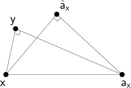 Figure 1
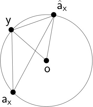 Figure 2