Entropy non-conservation and boundary conditions for Hamiltonian dynamical systems
Gerard McCaul, Alexander Pechen, Denys I. Bondar

TL;DR
This paper explores how boundary conditions influence entropy conservation in Hamiltonian systems, revealing classical-quantum distinctions and identifying conditions for entropy preservation through self-adjoint extensions.
Contribution
It introduces a framework using self-adjoint extensions to determine entropy conservation in classical mechanics and links boundary conditions to quantum tunneling effects.
Findings
Entropy is conserved only for specific probability distributions.
Nonconserving states can be interpreted as quantum tunneling.
Boundary conditions determine the classical-quantum transition.
Abstract
Applying the theory of self-adjoint extensions of Hermitian operators to Koopman von Neumann classical mechanics, the most general set of probability distributions is found for which entropy is conserved by Hamiltonian evolution. A new dynamical phase associated with such a construction is identified. By choosing distributions not belonging to this class, we produce explicit examples of both free particles and harmonic systems evolving in a bounded phase-space in such a way that entropy is nonconserved. While these nonconserving states are classically forbidden, they may be interpreted as states of a quantum system tunneling through a potential barrier boundary. In this case, the allowed boundary conditions are the only distinction between classical and quantum systems. We show that the boundary conditions for a tunneling quantum system become the criteria for entropy preservation in…
Click any figure to enlarge with its caption.
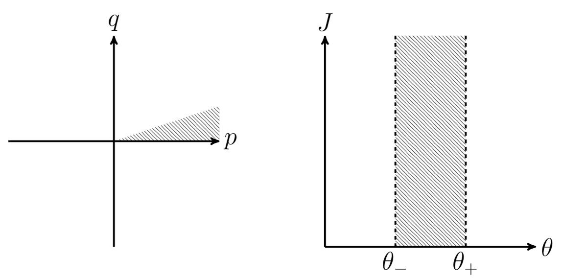 Figure 1
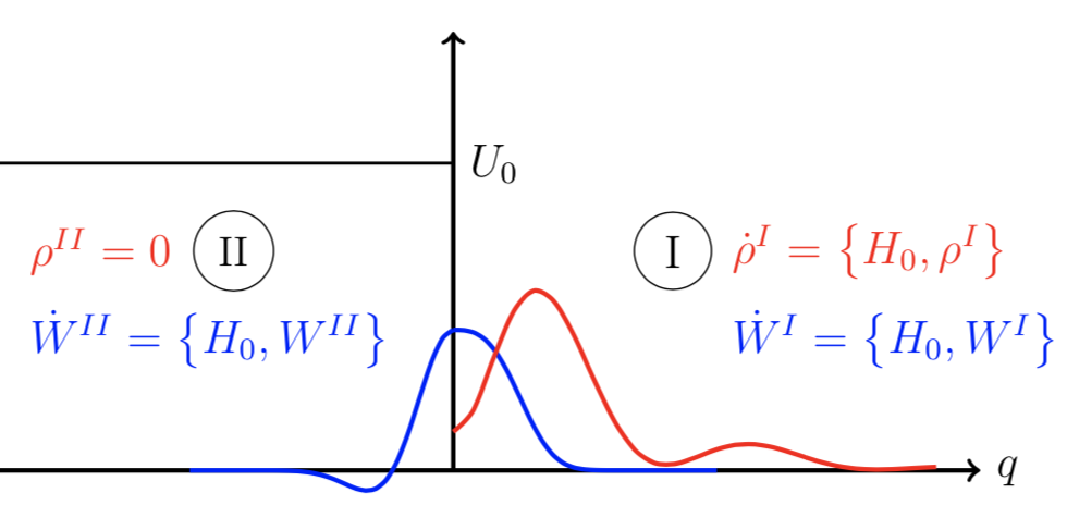 Figure 2
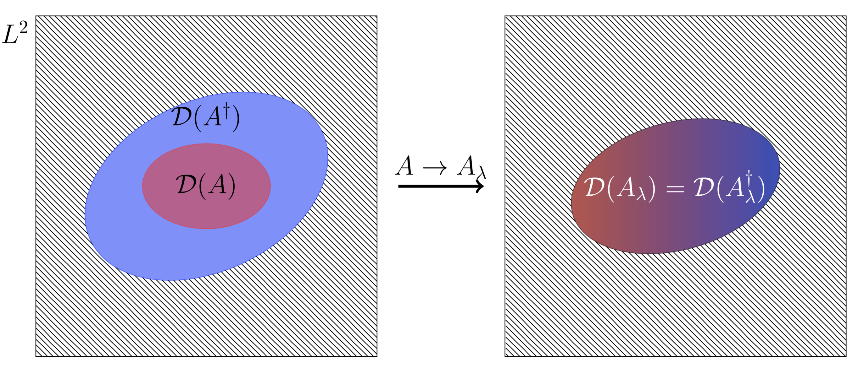 Figure 3
Peer Reviews
No public reviews on file for this paper yet. If you reviewed it on a platform where reviews are public (OpenReview, ICLR, NeurIPS, ICML), you can paste yours below so the community can read it here.
Videos
No videos yet. Explain this paper in a talk, walkthrough, or lecture? Add one.
Entropy non-conservation and boundary conditions for Hamiltonian dynamical systems
Gerard McCaul
Tulane University, New Orleans, LA 70118, USA
King’s College London, London WC2R 2LS, U.K.
Alexander Pechen
Steklov Mathematical Institute of Russian Academy of Sciences, Gubkina str. 8, Moscow 119991, Russia
National University of Science and Technology "MISIS", Leninski prosp. 4, Moscow 119049, Russia
Denys I. Bondar
Tulane University, New Orleans, LA 70118, USA
(March 2, 2024)
Abstract
Applying the theory of self-adjoint extensions of Hermitian operators to Koopman von Neumann classical mechanics, the most general set of probability distributions is found for which entropy is conserved by Hamiltonian evolution. A new dynamical phase associated with such a construction is identified. By choosing distributions not belonging to this class, we produce explicit examples of both free particles and harmonic systems evolving in a bounded phase-space in such a way that entropy is nonconserved. While these nonconserving states are classically forbidden, they may be interpreted as states of a quantum system tunneling through a potential barrier boundary. In this case, the allowed boundary conditions are the only distinction between classical and quantum systems. We show that the boundary conditions for a tunneling quantum system become the criteria for entropy preservation in the classical limit. These findings highlight how boundary effects drastically change the nature of a system.
I Introduction
Entropy is a critical element of physical theories, defining the notion of equilibrium (Lieb and Yngvason, 2000), as well as serving as a measure of irreversibility (Ford, 2015) and the arrow of time (Parrondo, den Broeck, and Kawai, 2009; Brown, Myrvold, and Uffink, 2009; Batalhão et al., 2015). In thermodynamics, the physical content of entropy is contained in its time dynamics, rather than its absolute value. Given the vital role which entropy plays in characterizing physical systems, the conditions under which entropy is time dependent are of great interest.
While entropy is an integral component of our understanding of thermodynamics and information, it is not a microscopic quantity and its definition therefore contains a degree of flexibility (Hanggi, Hilbert, and Dunkel, 2015). The entropy of a system depends on the level of course graining in the phase space, and on the variables considered (Jaynes, 1992). In this paper we shall adopt the Gibbs measure of entropy for a probability density of a one-dimensional system with coordinate and momentum ,
[TABLE]
which at equilibrium is equivalent to the thermodynamic entropy (Mackey, 1989).
It is often stated that, for a reversible process, the entropy change is zero. Another common assumption is that Hamiltonian systems are time reversible. The two ideas are often combined into the claim that systems with a Hamiltonian evolution conserve entropy. This is not in fact the case. The probability density of a Hamiltonian system evolves according to the Liouville equation
[TABLE]
Taking the time derivative of Eq. (1), substituting the Poisson bracket , and integrating this by parts, one finds that the entropy production arises solely from the boundary terms. For a system with box boundaries at , ,
[TABLE]
It is at this point that one generally assumes boundary conditions to kill these terms (Landau and Lifshitz, 1951), but this assumption is overly restrictive, and peculiar to both the dynamics and distribution which is being evolved. This assumption does not give a * general* answer to the question of entropy conservation. At the same time, it is difficult to assess how modifications, such as a restriction in phase space, would affect the entropy production.
To answer the question of entropy conservation with the greatest possible generality, we shall employ the Koopman von-Neumann (KvN) formalism. In particular, we shall use this formalism to reduce the problem of entropy conservation to the analysis of a classical self-adjoint evolution operator.
The theory of self-adjoint extensions of Hermitian operators is closely related to boundary conditions, and is vital in the resolution of apparent paradoxes in quantum mechanics (Bonneau, Faraut, and Valent, 2001). The theory also makes explicit connection to topological phases of matter (Chen, Lu, and Vishwanath, 2014; Chen et al., 2012; Ahari, Ortiz, and Seradjeh, 2016) and spontaneously broken symmetries (Araujo, Coutinho, and Fernando Perez, 2004; Berman, 1991; Capri, 1977). Moreover, self-adjointness assumes a vital role in novel approaches to prove the Riemann zeta hypothesis (Bender, Brody, and Müller, 2017). It is, in short, a useful formalism that may be applied to the problem of entropy conservation when alloyed to the KvN description of classical dynamics.
We proceed as follows: A brief overview of KvN mechanics is provided in Section II. Section III outlines the theory of self-adjoint operators necessary for our analysis, and the conditions under which a Hermitian operator is self adjoint. The equivalence of the criteria for a generator of time translations to be self-adjoint and for that evolution to conserve entropy is shown. Section IV applies the developed technique to a classical oscillator, and establishes the conditions for entropy conservation when its coordinate is restricted to the half-line (i.e., a phase space . Section V provides specific counterexamples of distributions evolved by Hamiltonian dynamics which violate entropy conservation. Section VI discusses in detail these entropy violating distributions, providing an interpretation of their physical significance and relation to quantum dynamics. Finally, Sec. VII concludes with a discussion of the results.
II Koopman-von Neumann Dynamics
KvN mechanics is the reformulation of classical mechanics in a Hilbert-space formalism (Koopman, 1931). This operational formalism underlies ergodic theory (Reed and Simon, 1980), and is a natural method for modeling quantum-classical hybrid systems (Sudarshan, 1976; Viennot and Aubourg, 2018; Bondar and Tronci, 2018). KvN dynamics has also been applied to establish a classical speed limit for dynamics(Okuyama and Ohzeki, 2018) and an alternate formulation of classical electrodynamics (Rajagopal and Ghose, 2016). By using the KvN formalism it is even possible to combine classical and quantum dynamics in a unified framework known as operational dynamical modeling (Bondar et al., 2012; Bondar, Cabrera, and Rabitz, 2013).
The KvN formalism has been successfully applied to construct both deterministic and stochastic classical path integrals (Gozzi, Cattaruzza, and Pagani, 2014; Shee, 2015), including generalizations with geometric forms (Gozzi and Reuter, 1994). These path integral formulations may be usefully applied with classical many-body diagrammatic methods (Liboff, 2003) and for the derivation and analysis of generalized Langevin equations (McCaul, 2018). KvN has been used to study specific phenomena, including examinations of dissipative behavior (Chruściński, 2006), linear representations of nonlinear dynamics (Brunton et al., 2016), analysis of the time-dependent harmonic oscillator (Ramos-Prieto et al., 2018), and other industrial applications (Mezić, 2005; Budišić, Mohr, and Mezić, 2012).
Both KvN and quantum dynamics begin by defining the Hilbert space :
[TABLE]
which is the set of all functions on the space that are square integrable with measure . In classical KvN dynamics is a phase space, while in quantum mechanics it is a configuration space. The inner product of the elements of this Hilbert space is
[TABLE]
for . The elements of are interpreted as (unnormalized) probability density amplitudes which obey the Born rule in both quantum and KvN mechanics (Brumer and Gong, 2006),
[TABLE]
In both cases, the dynamics of elements of are given by a one-parameter, strongly continuous group of unitary transformations on ,
[TABLE]
The form of this family of unitary transformations is, by Stones’ theorem (von Neumann, 1932a):
[TABLE]
where is a unique self-adjoint operator. Self-adjointness is a stronger condition than Hermiticity, and its necessity shall be demonstrated in Sec. III.1. The family of unitary transformations may be interpreted as time evolution, leading to the differential equation:
[TABLE]
Specifying the form of this operator adds physics to the formalism. For example, one may derive both quantum and classical dynamics from this model by defining a fundamental commutation relation and assuming that observable expectations obey the Ehrenfest theorems.
The sole distinction between Koopman dynamics and quantum mechanics is in the choice of commutation relations (Bondar et al., 2012). In the quantum case , and the self-adjoint operator is then , yielding:
[TABLE]
which is the familiar Schrödinger equation. In KvN dynamics, , and is the Koopman operator defined as
[TABLE]
This leads to the remarkable conclusion that probability density amplitudes are governed by the Liouville equation, in the same way as probability densities themselves:
[TABLE]
The choice of commutation relation also defines the measure on the Hilbert space. While is a valid measure in the classical case, only (in the coordinate representation) preserves non-negativity for the quantum commutation relation (Hamhalter, 2003). One may still use the full phase space quantum mechanically, but the object under consideration in this case is the Wigner quasiprobability distribution (Baker, 1958; Curtright, Fairlie, and Zachos, 2014; Groenewold, 1946).
It may appear at first glance that the KvN framework is a formal hammer cracking a classical nut, but this formulation provides a key advantage; one may exploit the deep theory of operators on Hilbert space. In particular, the theory of self-adjoint operators allows the same general statements to be made about entropy conservation as in the quantum case. Explicitly, if is self-adjoint, then the Gibbs entropy will be conserved. To prove this however, we must first review the definition of a self-adjoint operator.
III Criteria for Conservation of Entropy
III.1 Self-Adjoint Operators
An operator in the Hilbert space is a pair where is a linear mappings of elements in a subset of the Hilbert space onto ,
[TABLE]
The set is the domain of the operator, i.e., the set of vectors in the Hilbert space for which the operator mapping is defined. If the Hilbert space is finite, operators may be represented as finite matrices, and multiplication of a vector by a matrix is well defined for all vectors in a finite-dimensional Hilbert space, in this case (Akhiezer and Glazman, 1993). For infinite-dimensional Hilbert spaces however, this is not the case and the operator domain does not necessarily coincide with the full Hilbert space.
Assuming an operator is densely defined [i.e., is a dense subspace of ] (Reed and Simon, 1980), one may define its adjoint operator as follows. A vector belongs to the domain if and only if the linear functional is continuous. Then, by the Riesz representation theorem, there exists a unique such that for any . Action of the adjoint operator on is defined as . One has
[TABLE]
It may happen that the adjoint operator does not exist (its domain may not be dense or even empty; see, e.g., Example 4 in Sec. VIII.1, Vol. 1 of Ref. (Reed and Simon, 1980)). This occurs if the graph of the operator; that is, the set of pairs , , is not closable in . Otherwise the adjoint operator is correctly defined.
A Hermitian (or symmetric) (Reed and Simon, 1980) operator is such that and the action of the operator and its adjoint is identical on . Then
[TABLE]
In the special case the operator is called self-adjoint. The condition requires that the adjoint of a symmetric operator is defined for any element in , but does not otherwise restrict its domain. Figure 1 illustrates the fact that the domain of a symmetric operator on a Hilbert space is a subset of the domain of its adjoint operator.
To illustrate the difference between a Hermitian and self-adjoint operator, we evaluate a Koopman operator with domain
[TABLE]
The Hermitian property of this operator may be investigated by using integration by parts:
[TABLE]
If is Hermitian, the following boundary condition holds:
[TABLE]
which is automatically satisfied by using the example domain of Eq. (16). As a result, these boundary conditions for the wavefunction specify the operator’s domain.
For the example domain, the boundary condition is satisfied regardless of the domain of the adjoint operator, . This potential mismatch in the domains of an operator and its adjoint is deeply problematic, as it implies a violation of time-reversal invariance (Bonneau, Faraut, and Valent, 2001). For this reason, the generator of time-translations (and in fact all observable operators) must be self-adjoint, as defined above. Given an operator with a defined action, it is a nontrivial exercise to find which domains, if any, will make the operator self-adjoint. Fortunately, there is a powerful theorem of functional analysis that may be applied to this problem.
III.2 The von Neumann deficiency index theorem
The von Neumann deficiency index theorem (von Neumann, 1932b) can be used to answer the question of whether an operator may be made self adjoint. Details of this important theorem may be found in Refs. (Bonneau, Faraut, and Valent, 2001; Akhiezer and Glazman, 1993; Naimark, 2009), but we shall briefly outline its use here.
The deficiency index theorem determines all possibilities for a Hermitian operator with domain by considering the eigenstates in with imaginary eigenvalues, i.e., those satisfying the equation:
[TABLE]
The number of linearly independent solutions for are the deficiency indices . They determine the following three possibilities (Reed and Simon, 1980):
[TABLE]
A self-adjoint extension is an operator with the same action as on , but whose domain has been modified, , to enforce the self-adjoint condition. Figure 1 shows an example schematic, demonstrating the domain modification made by a self-adjoint extension.
If , each self adjoint extension is characterized by parameters, in the form of an unitary matrix . For the Koopman operator, the boundary condition corresponding to a self-adjoint extension with domain is simply Eq. (18), replacing with (Araujo, Coutinho, and Fernando Perez, 2004):
[TABLE]
Here is one of the solutions to Eq. (19) and is an element of the unitary matrix . Consequently, one may use the deficiency index theorem to characterize the most general boundary condition on for which is self-adjoint in terms of .
III.3 Self-Adjoint Operators and Entropy Conservation
While the von Neumann deficiency index theorem establishes the conditions under which is self-adjoint, this does not explicitly address the question of entropy conservation. We now demonstrate that a self-adjoint Koopman operator guarantees entropy conservation. First, define the operator 111In the quantum case, the trace of this operator is the von Neumann entropy. This similarly obeys an theorem when is evolved by a Lindblad equation (Alicki, 1979).:
[TABLE]
where
[TABLE]
Note that the operator is explicitly nonlinear; however, the proof of its time independence does not rely on linearity, as if is self-adjoint, then
[TABLE]
where in the final equality, we have exploited that is self-adjoint and all the traces are finite. Having demonstrated the time independence of the trace of , we now express it in the basis:
[TABLE]
Expanding this yields:
[TABLE]
and therefore
[TABLE]
Thus, we establish that is the entropy, and is conserved for self-adjoint . Note, however, that entropy conservation is not in itself a guarantee of unitary evolutions.
To summarize, entropy conservation is guaranteed when the Koopman operator is self-adjoint. The domain of the self-adjoint extensions may be determined by using the deficiency index theorem. This domain corresponds to the most general boundary conditions which conserve entropy for a given Hamiltonian.
Establishing the self-adjoint extensions of an operator is a nontrivial exercise, but the analysis is most straightforward in a system whose Koopman operator is functionally dependent on only one phase-space coordinate. Therefore, in the following we consider the specific examples of free and periodic systems in action-angle coordinates, but emphasize that this is a choice of computational convenience in applying generic arguments.
IV Entropy Conservation For Cyclic Systems
We now apply the results of the previous section to derive the most general entropy-preserving boundary conditions for both the harmonic oscillator and free particle with a bounded phase space. The first section will consider general box boundaries in action-angle coordinates.
IV.1 Self-adjoint domain In action-angle coordinates
Consider a system whose coordinates can be canonically transformed into a space where one coordinate is cyclic, i.e., a Hamiltonian that functionally depends on only one phase-space coordinate. Any periodic system may be described by these canonical action-angle coordinates (Goldstein, 2014), but here we take the simplest example of a harmonic oscillator:
[TABLE]
Using action-angle coordinates greatly simplifies the analysis, and can be achieved with the substitution:
[TABLE]
In the action-angle representation, we choose box phase-space boundaries, with and (see Fig. 2), which contains a particle restricted to the half-line as a special case. In the new coordinates, , leading to the following form of the Koopman operator for the harmonic oscillator:
[TABLE]
We now apply the deficiency index theorem in this new basis by finding the wavefunctions satisfying
[TABLE]
meaning that we look for solutions to
[TABLE]
Solutions to this equation have the form
[TABLE]
The solutions which belong to are all those for which:
[TABLE]
Any function satisfying determines a particular solution to . From this we conclude that .
Rather than apply Eq. (20) directly, in this case the Koopman operator has the same form as the quantum-mechanical momentum operator on a fixed interval. Following the examples of Refs. (Araujo, Coutinho, and Fernando Perez, 2004; Bonneau, Faraut, and Valent, 2001) we conclude that for each value of , the Koopman operator has a one parameter self-adjoint extension. Labeling each of these arbitrary parameters by , we find the boundary condition for the self-adjoint domain of :
[TABLE]
While this phase is not directly observable in expectations, it is gauge-invariant (in the sense of locally rotating a complete set of states).
Potential physical consequences of the choice of self-adjoint extension can be examined by observing that time evolution corresponds to a translation in . Including the time argument explicitly in the wavefunction, harmonic dynamics guarantee
[TABLE]
In particular, the wavefunction at the boundaries may be expressed in terms of a time translation of the wavefunction at an arbitrary point in
[TABLE]
Combining this with the fact that Eq. (34) must hold at all times, we obtain the relation
[TABLE]
where is an integer and . When is chosen to be , states may acquire an additional phase after each period of the motion. For this reason, although the dynamics are periodic, it is possible to choose boundary conditions such that the wavefunction is not periodically symmetric due to the additional phase. While observable expectations will be unaffected by such a phase, the time translation symmetry of correlation functions will be altered by its presence.
To demonstrate this, consider two observables and which have the two-time correlation function:
[TABLE]
where phase-space arguments on the right-hand side have been omitted for brevity. If one of the time arguments is shifted by the period of motion , the correlation function becomes
[TABLE]
Thus, the phase factor determining a self-adjoint extension has a nontrivial effect on time symmetries of observable correlations. This breaking of periodicity is in sharp contrast with correlation functions on the full phase space, where continuity of the wave function forces and hence .
The existence of a dynamical phase due to the boundary conditions is somewhat analogous to the Berry phase (Samuel and Bhandari, 1988) and its classical equivalent the Hannay angle (Hannay, 1985). The origin of these geometric phases is quite different, resulting from adiabatic holonomic variation of the Hamiltonian parameters. In both cases however, the naive expectation that the system will return to its original state (after either a single period of the motion, or returning to the original Hamiltonian parameters) is not always true. It is well known that, for the simple harmonic oscillator, the geometric phase change is zero (Usatenko, Provost, and Vallée, 1996), whereas here a phase may be acquired by the choice of boundary conditions.
IV.2 Entropy conservation on the half-line
Angular restrictions in the action-angle coordinate system may correspond to unphysical restrictions in the momentum subspace of the phase space. A restriction purely in the coordinate of phase space may be obtained by choosing the boundaries
[TABLE]
which leads to the half-line phase space in the original coordinates. The phase space is then and the Hilbert space is . Converting the wavefunction back to its original coordinates at the boundary we obtain
[TABLE]
which may be substituted into Eq. (34) to give the domain of self-adjoint evolutions on the half-line:
[TABLE]
Entropy preserving probability distributions therefore obey the condition
[TABLE]
which automatically satisfies Eq. (18).
This condition can be given a physical interpretation by considering the Liouville evolution as a continuity equation, where is the probability current in phase space:
[TABLE]
The probability current in the direction (integrated over ) is given by
[TABLE]
Substituting Eq. (43) into the above equation, we find that at the boundary,
[TABLE]
From this boundary condition, we conclude that the domain of states for self-adjoint Koopman operators corresponds precisely to a reflecting boundary condition at the boundary (Risken, 1989).
Finally, we note that there is no dependence in Eqs. (42) and (47). In the limit , the boundary condition for entropy preserving distributions is therefore unaffected, but the system Hamiltonian now describes a free particle rather than a harmonic oscillator. For this reason, Eq. (47) also describes the self-adjoint domain of the free particle.
V nonconserving States
Given the self-adjoint conditions derived in the previous section, one can construct a reasonable initial wavefunction (and hence probability density) on the half line which does not conserve entropy. Take for example the initial wavefunction
[TABLE]
where crucially, and the normalization factor is . The rate of entropy change for this state can be calculated directly from Eq. (3). For the free particle we have in the domain
[TABLE]
and for the harmonic oscillator in the same domain (setting )
[TABLE]
In both cases the entropy is nonconserved. The energy expectation and partition function for both systems are also time dependent. For this state the integrated boundary probability current is
[TABLE]
i.e., at the boundary the probability is being either partially absorbed or generated depending on the sign of .
VI Interpreting nonconserving States
To give an interpretation to the nonconserving states, we now consider the boundary conditions for a quantum-mechanical system in the full phase space . The dynamics are governed by the Hamiltonian H\left(q,p\right)=H_{0}\left(q,p\right)+U_{0}\Theta\text{\left(-q\right)}, where is the Hamiltonian for either a free-particle or harmonic oscillator, is the Heaviside step function, and is a constant that satisfies
[TABLE]
i.e., the U_{0}\Theta\text{\left(-q\right)} term represents a classically impenetrable barrier on the negative part of the real line.
We describe the quantum system with the wavefunction . This can be brought into contact with earlier results by using the Wigner distribution to describe the quantum system in phase space (Case, 2008):
[TABLE]
The Wigner distribution is a quasiprobability that captures quantum-mechanical expectations as a distribution over phase space, which in the classical limit becomes the classical wavefunction (Bondar et al., 2013). Here, the classical wavefunction refers to the wavefunction evolved according to KvN dynamics, i.e., from Secs. II-V.
For an arbitrary quantum operator its expectation may be described by using the Wigner distribution:
[TABLE]
where is the Wigner map of the operator :
[TABLE]
The Wigner distribution evolution is described by the Moyal bracket (Bondar et al., 2013):
[TABLE]
When the system Hamiltonian is at most quadratic in both the and coordinates (as is the case for the example Hamiltonians studied in Sec. IV), the Moyal bracket is simplified, and the Wigner distribution is evolved by the Poisson bracket (Case, 2008), in the same way as Eq. (2):
[TABLE]
Remarkably, in this case, the quantum Wigner distribution, classical probability distribution, and classical wave function *all *share the same equation of motion. In this scenario, quantum and classical systems are distinguished purely by the restrictions placed on them by their boundary conditions.
Labeling the positive half-line as region I and the negative half-line as region II (see Fig. 3), we consider a system initially confined to region I. By Eq. (50), it is impossible for a classical system to transition into region II. In this case the classical system is described by the phase space and the results of section IV.2 apply. Most importantly, Eq. (47) holds, meaning that at all times and .
For the quantum system, while the equation of motion for is identical to that for both the classical wave function and the associated probability density , a quantum state initially confined to region I may tunnel into the classically forbidden region II. For such a quantum system, the boundary condition between regions I and II is not described by Eq. (50), but must be generalized. This quantum boundary condition simply enforces continuity for the quantum wavefunction on the border between regions I and II (Griffiths, 2004):
[TABLE]
To account for this boundary condition, the Wigner distribution over the whole real-line is expressed piecewise
[TABLE]
The quantum boundary conditions can then be expressed in terms of the Wigner function with (Case, 2008)
[TABLE]
and
[TABLE]
Substituting these expressions into the quantum boundary conditions of Eqs. (56) and (57), yields these boundary conditions in terms of Wigner distributions:
[TABLE]
where the left-hand side of the second boundary condition is the Wigner flow (Steuernagel, Kakofengitis, and Ritter, 2013; Oliva, Kakofengitis, and Steuernagel, 2018) over the boundary, defined in the same way as Eq. (47). Focusing exclusively on region I, the current boundary condition is:
[TABLE]
Here is some functional dependent only on the Wigner distribution of region II. This boundary condition is the only feature that distinguishes from the classical system described by . Furthermore, in the classical limit, and (for a system initially confined to region I), . In this case Eq. (63) is equivalent to Eq. (47), recovering the classical boundary condition.
Equation (63) also allows one to interpret the entropy nonconserving states in Sec. V. These states are characterized by . While this violates the classical boundary condition, if is interpreted instead as , then the non-zero integrated current is consistent with Eq.(63). Hence, for the free-particle and harmonic oscillator, the entropy nonconserving states in a classical system with a classically impassible potential barrier are partial solutions for a quantum system tunneling through the barrier.
Finally, we note that the arguments presented in this section may be applied to the phenomenon of reflection above a barrier. This is another purely quantum effect, which may be regarded as tunneling through a momentum space barrier (Jaffe, 2010). Performing an analogous classical analysis for a harmonic system restricted to the half-line in momentum space, a similar relationship between allowed states and boundary conditions can be obtained, where classically forbidden reflected Wigner distributions match entropy nonconserving states of the classical system.
VII Conclusions
We have applied the Koopman von Neumann formalism to reduce the problem of entropy conservation in a classical system to the problem of identifying self-adjoint extensions of the Koopman operator. In this way, one can explore for a given system the full range of admissible, physical probability distributions and phase-space restrictions which preserve entropy. Applying this technique to the harmonic oscillator and free particle, a relationship between the choice of self-adjoint extension and the boundary condition was determined. In the case of the harmonic oscillator, this choice is reflected in the breaking of the periodic symmetry of correlation functions. This demonstrates a new class of situations where self-adjoint extensions of operators play an important role in distinguishing subtle phenomena.
In the example cases studied, it was possible to construct apparently reasonable states in the phase space which do not belong to the domain of a self-adjoint Koopman operator, and consequently do not preserve entropy. These states were interpreted using the fact that the restricted phase space for the classical system corresponds to a classically impenetrable potential barrier, but a quantum system may tunnel into this forbidden region.
For both the free particle and harmonic oscillator, quantum and classical dynamical equations coincide, and the two regimes are distinguished purely by the allowed boundary conditions. This allowed for the interpretation of entropy nonconserving classical states as partial descriptions of tunneling quantum states. Additionally, this approach demonstrated that the classical boundary condition corresponding to a self-adjoint Koopman operator is the classical limit of the quantum boundary condition for a tunneling state.
These results highlight the importance of boundary conditions for fundamental aspects of Hamiltonian evolution. While Hamilton’s equations of motion provide a local description of the dynamics, the entropy provides a global characterization of the evolution, and is therefore sensitive to the self-adjointness of the Koopman operator. Even in the case that equations of motion are formally time-reversal symmetric, the choice of boundary condition can break entropy preservation, and thus time-reversal symmetry.
Acknowledgements.
The authors would like to thank the referees for their valuable comments, which have inspired a number of the results presented here. D.I.B. is grateful to Jean-Luc Cambier for suggesting a research direction that has directly led to this work. G.M. and D.I.B. are supported by Air Force Office of Scientific Research Young Investigator Research Program (FA9550-16-1-0254). A.P. is supported by project No. 1.669.2016/1.4 of the Ministry of Science and Higher Education of the Russian Federation.
The reference list from the paper itself. Each links out to its DOI / PubMed record.
- 1Lieb and Yngvason (2000) E. H. Lieb and J. Yngvason, Phys. Today 53 , 32 (2000) . · doi ↗
- 2Ford (2015) I. J. Ford, New J. Phys. 17 , 075017 (2015) . · doi ↗
- 3Parrondo, den Broeck, and Kawai (2009) J. M. R. Parrondo, C. V. den Broeck, and R. Kawai, New J. Phys. 11 , 73008 (2009) .
- 4Brown, Myrvold, and Uffink (2009) H. R. Brown, W. Myrvold, and J. Uffink, Stud. Hist. Philos. Sci. 40 , 174 (2009) , ar Xiv:0809.1304 . · doi ↗
- 5Batalhão et al. (2015) T. B. Batalhão, A. M. Souza, R. S. Sarthour, I. S. Oliveira, M. Paternostro, E. Lutz, and R. M. Serra, Phys. Rev Lett. 115 , 190601 (2015) , ar Xiv:1502.06704 . · doi ↗
- 6Hanggi, Hilbert, and Dunkel (2015) P. Hanggi, S. Hilbert, and J. Dunkel, Philos. Trans. Royal Soc. A 374 (2015).
- 7Jaynes (1992) E. E. T. Jaynes, in Maximum entropy and Bayesian methods , Vol. 17 (Springer, 1992) pp. 1–21. · doi ↗
- 8Mackey (1989) M. C. Mackey, Rev. Mod. Phys. 61 , 981 (1989) . · doi ↗