Scaling and spatial intermittency of thermal dissipation in turbulent convection
Shashwat Bhattacharya, Ravi Samtaney, and Mahendra K. Verma

TL;DR
This paper derives scaling laws for thermal dissipation in turbulent convection, revealing boundary layer dominance and suppression of bulk dissipation, with numerical simulations confirming stretched exponential distributions.
Contribution
It introduces new scaling relations for thermal dissipation in turbulent convection at various Prandtl numbers, supported by direct numerical simulations.
Findings
Boundary layer dissipation dominates over bulk dissipation.
Thermal dissipation in the bulk is suppressed compared to passive scalar dissipation.
Dissipation rate distributions follow stretched exponential functions.
Abstract
We derive scaling relations for the thermal dissipation rate in the bulk and in the boundary layers for moderate and large Prandtl number (Pr) convection. Using direct numerical simulations of Rayleigh-B\'{e}nard convection, we show that the thermal dissipation in the bulk is suppressed compared to passive scalar dissipation. The suppression is stronger for large Pr. We further show that the dissipation in the boundary layers dominates that in the bulk for both moderate and large Pr. The probability distribution functions of thermal dissipation rate, both in the bulk and in the boundary layers, are stretched exponential, similar to passive scalar dissipation.
Click any figure to enlarge with its caption.
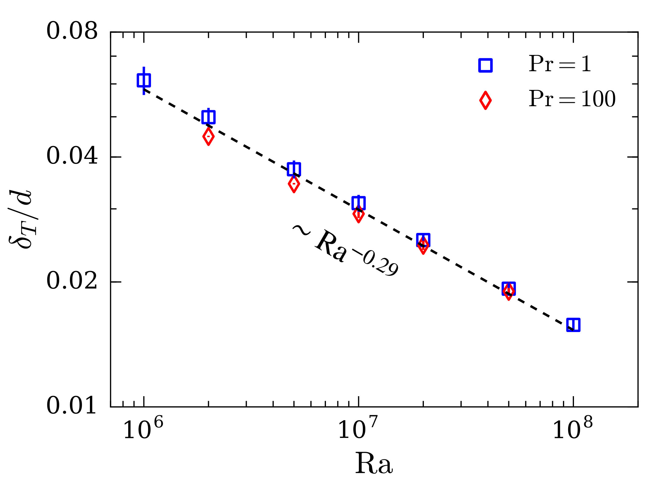 Figure 1
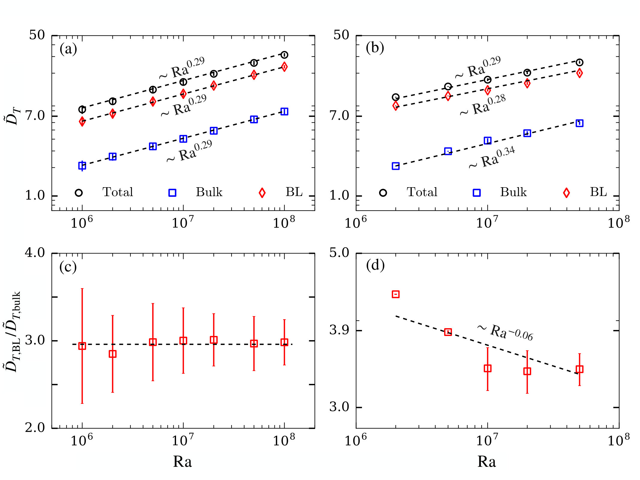 Figure 2
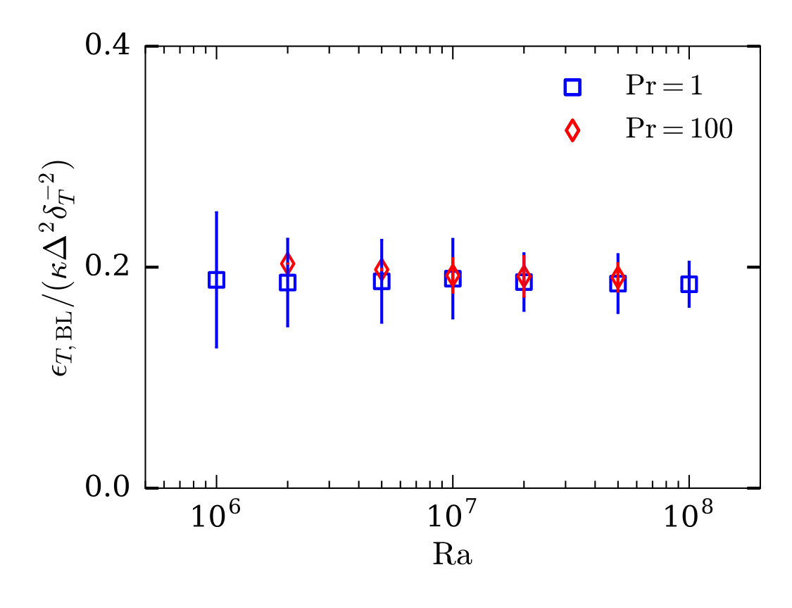 Figure 3
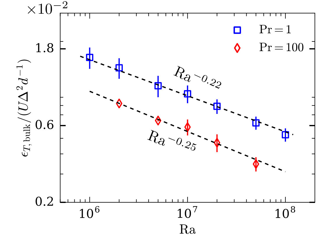 Figure 4
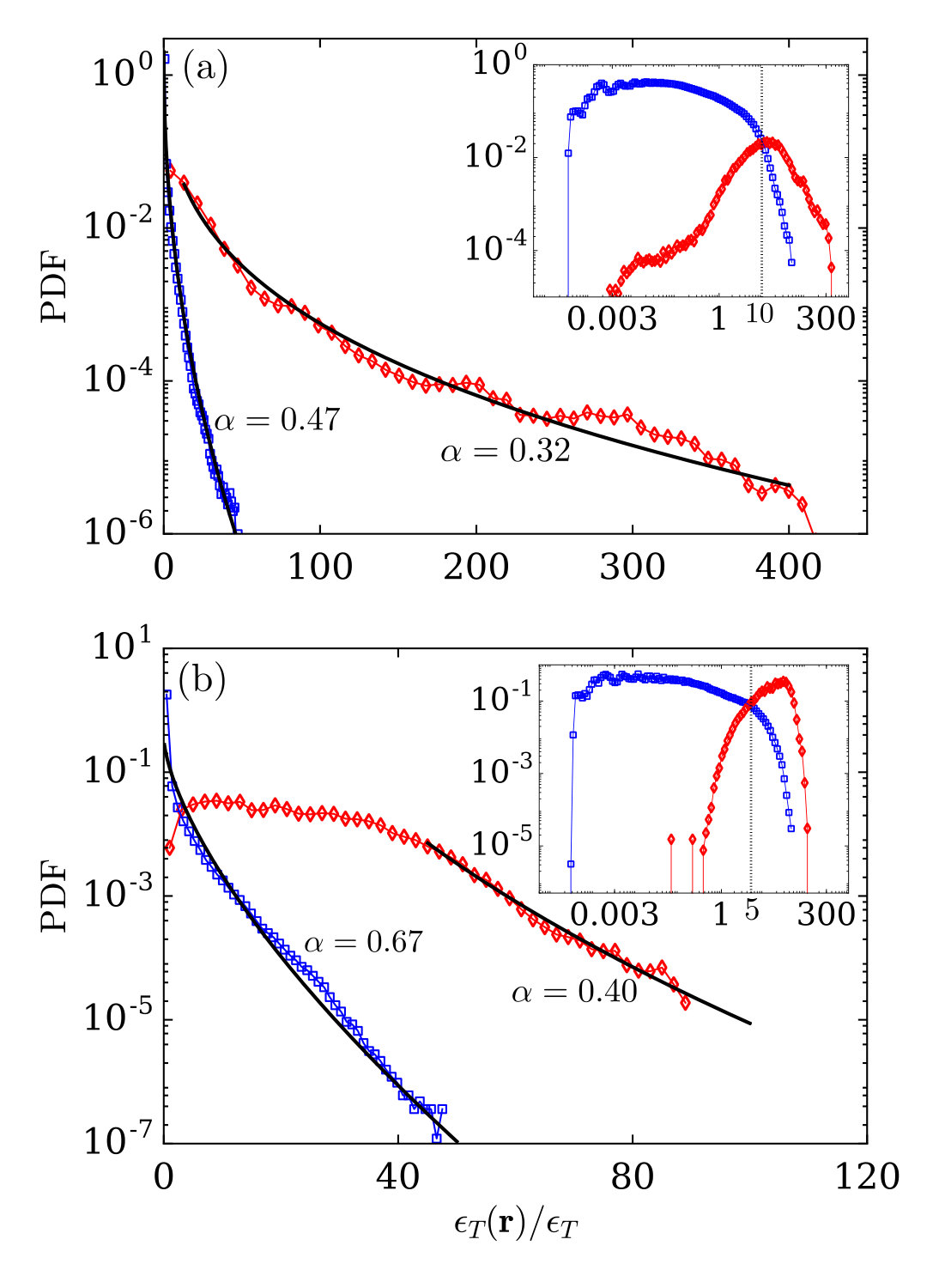 Figure 5
| Snapshots | |||||||||
|---|---|---|---|---|---|---|---|---|---|
Peer Reviews
No public reviews on file for this paper yet. If you reviewed it on a platform where reviews are public (OpenReview, ICLR, NeurIPS, ICML), you can paste yours below so the community can read it here.
Videos
No videos yet. Explain this paper in a talk, walkthrough, or lecture? Add one.
Scaling and spatial intermittency of thermal dissipation in turbulent convection
Shashwat Bhattacharya
Department of Mechanical Engineering, Indian Institute of Technology Kanpur, Kanpur 208016, India
Ravi Samtaney
Mechanical Engineering, Division of Physical Science and Engineering, King Abdullah University of Science and Technology, Thuwal 23955, Saudi Arabia
Mahendra K. Verma
Department of Physics, Indian Institute of Technology Kanpur, Kanpur 208016, India
(17 June 2019)
Abstract
We derive scaling relations for the thermal dissipation rate in the bulk and in the boundary layers for moderate and large Prandtl number (Pr) convection. Using direct numerical simulations of Rayleigh-Bénard convection, we show that the thermal dissipation in the bulk is suppressed compared to passive scalar dissipation. The suppression is stronger for large Pr. We further show that the dissipation in the boundary layers dominates that in the bulk for both moderate and large Pr. The probability distribution functions (PDFs) of thermal dissipation rate, both in the bulk and in the boundary layers, are stretched exponential, similar to passive scalar dissipation.
pacs:
47.27.te, 47.27.-i, 47.55.P-
I Introduction
Scalar fields, such as temperature and concentration, are often carried along by turbulent flows. Flows with scalars are ubiquitous and frequently encountered in engineering and atmospheric applications. In general, these scalar fields influence the dynamics of fluid flow. The resulting coupling between the momentum and the scalar equations, along with strong nonlinearities, makes such flows very complex. Obukhov (1949) and Corrsin (1951) described the energetics of a simplified system consisting of homogeneous isotropic turbulence with passive scalar fields; such scalars do not affect the velocity field. In passive scalar turbulence, both kinetic energy [defined as ] and scalar energy [defined as ] are supplied at large scales. Here, and are scalar and velocity fields respectively, and denotes volume average. The supplied kinetic and scalar energies cascade to intermediate scales and then to dissipative scales. Similar to kinetic energy in homogeneous turbulence, the rate of scalar energy supply equals the scalar energy cascade rate and the scalar dissipation rate Lesieur (2008); Verma (2018). Dimensional analysis gives , where , , and are large-scale length, velocity, and scalar respectively.
In the present work, we consider turbulence in buoyancy-driven convection, which is an example of active scalar turbulence where the scalar field (temperature) influences the flow-dynamics. We focus on an idealized system called Rayleigh–Bénard convection (RBC) in which a fluid is enclosed between two horizontal walls, with the bottom wall being hotter than the top one. Ahlers, Grossmann, and Lohse (2009); Lohse and Xia (2010); Verma, Kumar, and Pandey (2017). Each horizontal wall is isothermal. RBC is specified by two nondimensional parameters—Rayleigh number () and Prandtl number (). These parameters are defined as
[TABLE]
where , , and respectively are the thermal expansion coefficient, kinematic viscosity, and thermal diffusivity of the fluid, is the gravitational acceleration, and and respectively are the temperature difference and the distance between the top and bottom plates.
The energetics of thermally-driven convection is more complex than that of passive scalar turbulence; this is due to the two-way coupling between the governing equations of momentum and thermal energy (see Sec. II), along with the presence of thermal boundary layers. Presently, we focus on the properties of thermal dissipation rate , where is the temperature field. In RBC, the volume-averaged thermal dissipation rate is related to the Nusselt number () by the following relation derived by Shraiman and Siggia (1990):
[TABLE]
The Nusselt number is the ratio of the total heat flux and the conductive heat flux, and is the Péclet number. When the thermal boundary layers are less significant than the bulk (as in the ultimate regime proposed by Kraichnan Kraichnan (1962)), or absent (as in a periodic boxVerma et al. (2012)), both Nu and Pe are proportional to (See Refs.Grossmann and Lohse (2000, 2001); Verma, Kumar, and Pandey (2017)). These relations, when substituted in Eq. (1), yield , similar to passive scalar turbulence.
In RBC, the thermal boundary layers near the conducting walls play an important role in the scaling of thermal dissipation rate. In our present work, we focus on the dependence of thermal dissipation rate and other quantities. For moderate Prandtl numbers (of order 1), it has been shown via scaling arguments Malkus (1954); Castaing et al. (1989); Grossmann and Lohse (2000, 2002), experiments Castaing et al. (1989); Qiu and Tong (2002); Qiu et al. (2004); Brown, Funfschilling, and Ahlers (2007); Funfschilling et al. (2005); Nikolaenko et al. (2005); He et al. (2012); Ahlers et al. (2012); Vial and Hernándes (2017), and numerical simulations Verzicco and Camussi (2003); Scheel, Kim, and White (2012); Scheel and Schumacher (2014); Waleffe, Boonkasame, and Smith (2015); Verma, Ambhire, and Pandey (2015); Zhou and Chen (2018); Pandey and Verma (2016); Pandey et al. (2016) that
[TABLE]
Note that the exponents in the above expressions shown here are approximate. Substitution of these expressions in Eq. (1) yields
[TABLE]
When compared to passive scalar flow, the additional term in RBC accounts for suppression of nonlinear interactions due to the presence of walls; Pandey and Verma (2016) and Pandey et al. (2016) showed that in RBC, the ratio of the non-linear term to the diffusive term in the equation for thermal energy is proportional to instead of Pe. The walls truncate some of the Fourier modes, resulting in several channels of nonlinear interations and energy cascades to be blocked (See Ref. Verma (2018) for details). Consequently, thermal dissipation in RBC is weakened compared to free passive scalar turbulence. For large Pr, Pandey and Verma (2016) and Pandey et al. (2016) have shown that instead of .
To better understand the effects of walls, we need to study the behavior of thermal dissipation separately in the boundary layers and in the bulk. It is generally believed that dissipation (thermal or viscous) occurs predominantly in the boundary layers Puthenveettil and Arakeri (2005); Puthenveettil, Ananthakrishna, and Arakeri (2005). However, phenomenological arguments and numerical results presented by Verma, Kumar, and Pandey (2017) imply that significant dissipation occurs also at large scales, i.e., in the bulk. Motivated by this, Bhattacharya et al. Bhattacharya et al. (2018) computed the viscous dissipation rate separately in the bulk and in the boundary layers for moderate Pr. Interestingly, they found the bulk dissipation to be greater, albeit marginally, than the boundary layer dissipation. On the other hand, the thermal dissipation for moderate Pr convection was shown to be dominant in the boundary layers; refer to Verzicco and Camussi Verzicco and Camussi (2003) and Zhang, Zhou, and Sun (2017).
In this paper, we conduct a more detailed analysis of thermal dissipation rate in the bulk and boundary layers for not only moderate Pr but also for large Pr convection. Note that the statistics of thermal dissipation for large Pr are less explored in literature. We compare and quantify the total and average thermal dissipation rates in the bulk and in the boundary layers using scaling arguments and numerical simulations. We also examine the probability distribution functions of the thermal dissipation in these regions. Our analysis is similar to that conducted by Bhattacharya et al. (2018) on viscous dissipation rate.
The outline of the paper is as follows. In Sec. II, we present the governing equations of RBC along with their nondimensionalization. We discuss the numerical method in Sec. III. In Sec. IV, we compute the thermal boundary layer thickness and present scaling arguments for the thermal dissipation rate in the bulk and in the boundary layers. We verify these scaling relations using our numerical results. We also study the spatial intermittency of thermal dissipation rate. Finally, we conclude in Sec. V.
II Governing Equations
In RBC, under the Boussinesq approximation, the thermal diffusivity () and the kinematic viscosity () are treated as constants. The density of the fluid is considered to be a constant except for the buoyancy term in the governing equations. Further, the viscous dissipation term is considered to be small and is therefore dropped from the temperature equation. The governing equations of RBC are as followsChandrasekhar (2013); Verma (2018):
[TABLE]
where and are the velocity and pressure fields respectively, is the temperature field with respect to a reference temperature, is the thermal expansion coefficient, is the mean density of the fluid, and is acceleration due to gravity.
Using as the length scale, as the velocity scale, and as the temperature scale, we non-dimensionalize Eqs. (3)-(5), which yields
[TABLE]
In Sec. III, we describe the numerical method used for our simulations.
III Numerical Method
We conduct our numerical analysis for (i) and (ii) fluids. For , we use the simulation data of Bhattacharya et al. (2018) and Kumar and Verma (2018), which were obtained using the finite volume code OpenFOAM Jasak et al. (2007). The simulations were conducted on a grid for Ra ranging from to . No-slip boundary conditions were imposed at all the walls, isothermal boundary conditions at the top and bottom walls, and adiabatic boundary conditions at the sidewalls. For time marching, second-order Crank-Nicholson scheme was used. For , we conduct fresh simulations following the aforementioned schemes, boundary conditions, and grid resolution for Ra’s ranging from to . A constant time-step was chosen, with and , depending on the parameters (see Table 1 for details). Here, corresponds to .
We ensure that a minimum of 8 grid points is in the thermal boundary layers, thereby satisfying the resolution criterion set by Grötzbach (1983) and Verzicco and Camussi (2003). In RBC, the thermal boundary layer thickness is defined as the distance between the wall and the point where the tangent to the planar-averaged temperature profile near the wall intersects with the average bulk temperature line Ahlers, Grossmann, and Lohse (2009); Scheel, Kim, and White (2012); Shi, Emran, and Schumacher (2012); Scheel and Schumacher (2014). To ensure that the smallest length scales are resolved, we note that the ratio of the Batchelor length scale Batchelor (1959) to the maximum mesh width remains greater than unity for all runs. The only exception is for , case where , which is marginally less than unity. The Nusselt numbers computed using our data are consistent with those obtained in other simulations of RBC for the same geometry Wagner and Shishkina (2013); Pandey and Verma (2016); Pandey et al. (2016); this is how we validate our data. Further, the Nusselt numbers computed numerically using match closely with those computed using and Eq. (1). This is further validates our simulations. See Table 1 for the comparison of these two Nusselt numbers. All the quantities analyzed in this work are time-averaged over 40-100 snapshots after attaining steady-state (see Table 1).
In the Sec. IV, we discuss the numerical results, focussing on the scaling of the thermal dissipation rate in the bulk and in the boundary layers, their relative contributions to the total thermal dissipation rate, and their spatial intermittency.
IV Numerical Results
IV.1 Boundary layer thickness
Using the simulation results, we first compute the thickness of the thermal boundary layers. Theoretically, boundary layer thickness () is related to the Nusselt number as Ahlers, Grossmann, and Lohse (2009)
[TABLE]
Now, as discussed in Sec. I, for of order 1. Numerical simulations Pandey, Verma, and Mishra (2014); Pandey and Verma (2016); Pandey et al. (2016) reveal that for large Pr as well. Therefore, for both and , we expect
[TABLE]
We numerically compute ’s using the planar averaged temperature profile and list them in Table 1. Further, we plot them versus Ra in Figs. 1(a) and (b) for both and . The best-fit curves of the data yield
[TABLE]
with the error in the exponents being approximately . The obtained fit is reasonably consistent with Eq. (10).
IV.2 Scaling of thermal dissipation rate
In this subsection, we study the scaling of average thermal dissipation rate in the bulk () and in the boundary layers () using our numerical data. These quantities are dissipation per unit volume. Based on these, using scaling arguments, we predict the relations for the total dissipation rate in the bulk () and in the boundary layers (), which are the products of average thermal dissipation rates in these regions and their corresponding volumes. We verify their scaling relations using our simulation data and analyze the relative strength of the bulk and the boundary layer dissipation.
IV.2.1 Bulk dissipation
Using our simulation data, we numerically compute and the large-scale mean flow . In deriving their unifying scaling theory, Grossmann and Lohse Grossmann and Lohse (2000, 2001) argued that . However, from our numerical data, we observe that
[TABLE]
instead of (see Fig. 2). The errors in the exponents are 0.02 and 0.01 for and respectively. Thus, the thermal dissipation in the bulk in RBC scales similar to the dissipation in the entire volume, and is distinctly weaker than that in passive scalar turbulence. For moderate Pr fluids, the decrease of with Ra has also been observed by Emran and Schumacher (2008) and Verzicco and Camussi (2003) for convection in a cylindrical cell, and by Zhang, Zhou, and Sun (2017) for two-dimensional RBC. As discussed in Sec. I, the walls suppress nonlinear interactions in RBC Pandey and Verma (2016); Pandey et al. (2016), consequently weakening the thermal dissipation rate at large scales. Note that Bhattacharya et al. (2018) observed similar suppression of viscous dissipation in the bulk, where instead of for .
The aforementioned suppression has an important implication in the scaling of the total thermal dissipation in the bulk (). The bulk volume can be approximated as
[TABLE]
because (see Table 1). We will now derive the scaling relations for separately for and .
: Using Eqs. (12) and (13), we write the following for the bulk dissipation:
[TABLE]
By multiplying the numerator and the denominator of the rightmost expression in Eq. (14) by , we rewrite as
[TABLE]
where is the Péclet number. As discussed in Sec. I, for moderate Pr. Substituting this relation in Eqs. (14) and (15), we obtain
[TABLE] 2. 2.
: Applying a similar procedure, we can write the total dissipation in the bulk for as
[TABLE]
because in this case. Now, according to the predictions of Grossmann and Lohse (2001) and Shishkina et al. (2017) for large Pr convection, . Pandey, Verma, and Mishra (2014), Pandey and Verma (2016), and Pandey et al. (2016) have also shown that for large Pr, . Substituting this relation in Eq. (17), we obtain
[TABLE]
Thus, the suppression of thermal dissipation in the bulk leads to a weaker dependence of the total thermal dissipation with Ra. Note that in the absence of this suppression, \tilde{D}_{T,\mathrm{bulk}}\sim{\color[rgb]{0,0,0}(\kappa\Delta^{2}d)}\mathrm{Pe}. Had this been the case, , normalized with , would have been proportional to for and for .
IV.2.2 Boundary layer dissipation
The heat transport in the boundary layers is primarily diffusive due to steep temperature gradients. Thus, we expect the thermal dissipation in the boundary layers to be given by
[TABLE]
We verify this by plotting the numerically computed versus in Fig. 3, where we observe the slope to be flat. For and at lower Ra, however, there is a very slight decrease of with Ra. However, we will ignore this in our scaling analysis.
The total thermal dissipation in the boundary layers is given by . Substituting Eq. (19) in the above relation and noting that , we obtain
[TABLE]
As discussed in Sec. IV.1, for and for . Substituting these relations in Eq. (20), we obtain
[TABLE]
IV.2.3 Ratio of the boundary layer and the bulk dissipation
To analyze the relative strengths of the thermal dissipation in the bulk and in the boundary layers, we divide Eq. (21) with Eqs. (16) and (18) to obtain the ratio of the total dissipation in the boundary layers and the bulk for and respectively. The predicted ratio is
[TABLE]
Thus, we expect the ratio of the boundary layer and bulk dissipation to have a weak dependence on Ra. For , this ratio remains approximately constant, implying that the relative strengths of the bulk and the boundary layer dissipation remain roughly invariant with Ra. However, for , the above ratio decreases weakly with Ra; this implies that the relative strength of the boundary layer dissipation decreases with Ra and that of the bulk dissipation increases with Ra. The magnitudes of the prefactors in Eq. (22) determine whether the bulk or the boundary layer dissipation is dominant. These prefactors are obtained using numerical simulations.
IV.2.4 Numerical verification of the scaling arguments
We numerically verify the scaling relations predicted by Eqs. (16), (18), (21), and (22). We compute (the total dissipation in the entire volume), , and using our simulation data and plot them versus Ra in Fig. 4(a) for and in Fig. 4(b) for . Our data fits well with following expressions:
[TABLE]
where . The errors in the exponents in the above expressions range from 0.001 to 0.02. The above expressions match with the scaling arguments presented in Eqs. (21), (16), and (18) within the fitting error.
The computed ratio of the boundary layer and the bulk dissipation is
[TABLE]
which agrees well with Eq. (22). We plot this ratio in Fig. 4(c) for and Fig. 4(d) for .
Because of the prefactors in Eq. (26), the ratio of the boundary layer and the bulk dissipation remains above unity, implying that the boundary layer dissipation is larger than the bulk dissipation, although they are of the same order. As shown in Figs. 4(c) and 4(d), the boundary layer dissipation is approximately 3-4 times greater than the bulk dissipation. This is unlike viscous dissipation for , where the dissipation in the bulk is greater, albeit marginally, than that in the boundary layers Bhattacharya et al. (2018). This is because while the temperature is fairly constant in the bulk (except for a few regions of localized plumes), the velocity in the bulk is not so, as illustrated in Fig. 5. Here, we show the temperature density plot superimposed with velocity vector plot on - plane at , for , . Clearly, the velocity fluctuations are large near the walls (just outside the viscous boundary layers) but small near the center. On the other hand, in the bulk. Thus, the velocity gradients in the bulk are more pronounced than the temperature gradients; this results in stronger viscous dissipation compared to thermal dissipation in the bulk. However, one must note that for , the viscous boundary layers will occupy almost the entire volume; thus the viscous dissipation in the boundary layers will be dominant. Also, we need to carefully simulate low Pr convection to find out whether bulk or boundary layer dissipation dominates in this regime.
The dominance of the total thermal dissipation in the boundary layers has been reported previously for convection in a slender cylindrical cell Verzicco and Camussi (2003) and for two-dimensional convection Zhang, Zhou, and Sun (2017).
IV.3 Spatial intermittency of thermal dissipation rate
In this subsection, we will study the intermittency of the local thermal dissipation rate . Since (see Fig. 1), the boundary layers occupy a much smaller volume than the bulk. Therefore, is much stronger in the boundary layers than in the bulk.
We compute the probability distribution functions (PDF) of in the entire volume, bulk and boundary layers to quantify the spatial intermittency of thermal dissipation rate. The PDFs are computed for for both and 100. We plot these quantities in Fig. 6(a) for and in Fig. 6(b) for . From the inset of Fig. 6(a), we observe that for , for , while for . This clearly shows that thermal dissipation is weak in the bulk and strong in the boundary layers. We observe a similar behaviour for Pr=100, but with cut-off [see the inset of Fig. 6(b)].
It has been analytically shown by Chertkov, Falkovich, and Kolokolov (1998) that the passive scalar dissipation has a stretched exponential distribution. This profile is given by for . Interestingly, the PDFs of thermal dissipation for RBC are also stretched exponential for both bulk and boundary layers. Our observation is consistent with earlier studies Emran and Schumacher (2008); He and Tong (2009); Zhang, Zhou, and Sun (2017). For bulk dissipation, the stretching exponent for , and for . The corresponding exponents for the boundary layers are 0.32 and 0.40 respectively.
Clearly, for both Pr, the tails of the PDFs are stretched more for the boundary layer dissipation. This is expected because extreme events are more frequent in the boundary layers than in the bulk; note that is stronger in the boundary layers. Further, for both bulk and boundary layer dissipation, ’s are smaller for . Thus, the tails of the PDFs are stretched more for , implying stronger spatial intermittency of thermal dissipation for the lower Pr fluid. This is because for Pr=1, convection is more turbulent than that for Pr=100, causing the temperature fluctuations to be more pronounced for the former.
V Conclusions
In this paper, we present scaling relations for thermal dissipation rate in the bulk and in the boundary layers in turbulent convection. Using numerical simulations of RBC, we show that compared to passive scalar turbulence, the thermal dissipation rate in the bulk is suppressed by a factor of for and for . Further, unlike viscous dissipation, the total thermal dissipation in the boundary layers is greater than that in the bulk. The ratio of the boundary layer and the bulk dissipation is roughly constant for , and decreases weakly with Ra for .
We also show that the probability distribution functions of thermal dissipation rate, both in the bulk and in the boundary layers, are stretched exponential, similar to passive scalar dissipation. The stretching exponent for the PDFs of boundary layer dissipation is lower than that of bulk dissipation, implying that extreme events occur more often in the boundary layers than in the bulk. We also show that the spatial intermittency of thermal dissipation is stronger for lower Pr fluids.
The results presented in this paper are important for modelling thermal convection. For example, we may need to incorporate the suppression of thermal dissipation in the bulk in the scaling analysis for Pe and Nu. Thus far, our analysis has been for . We need to extend them to low Pr convection for a comprehensive modelling of thermal convection.
Acknowledgements
We thank A. Pandey, A. Guha, and R. Samuel for useful discussions. Our numerical simulations were performed on Shaheen II at Kaust supercomputing laboratory, Saudi Arabia, under the project k1052. This work was supported by the research grants PLANEX/PHY/2015239 from Indian Space Research Organisation, India, and by the Department of Science and Technology, India (INT/RUS/RSF/P-03) and Russian Science Foundation Russia (RSF-16-41-02012) for the Indo-Russian project.
The reference list from the paper itself. Each links out to its DOI / PubMed record.
- 1Obukhov (1949) A. M. Obukhov, “Structure of the temperature field in a turbulent flow,” Isv. Geogr. Geophys. Ser. 13 , 58–69 (1949).
- 2Corrsin (1951) S. Corrsin, “On the spectrum of isotropic temperature fluctuations in an isotropic turbulence,” J. Appl. Phys. 22 , 469–473 (1951).
- 3Lesieur (2008) M. Lesieur, Turbulence in Fluids (Springer-Verlag, Dordrecht, 2008).
- 4Verma (2018) M. K. Verma, Physics of Buoyant Flows (World Scientific, Singapore, 2018).
- 5Ahlers, Grossmann, and Lohse (2009) G. Ahlers, S. Grossmann, and D. Lohse, “Heat transfer and large scale dynamics in turbulent Rayleigh-Bénard convection,” Rev. Mod. Phys. 81 , 503–537 (2009).
- 6Lohse and Xia (2010) D. Lohse and K.-Q. Xia, “Small-scale properties of turbulent Rayleigh–Bénard convection,” Annu. Rev. Fluid Mech. 42 , 335–364 (2010).
- 7Verma, Kumar, and Pandey (2017) M. K. Verma, A. Kumar, and A. Pandey, “Phenomenology of buoyancy-driven turbulence: recent results,” New J. Phys. 19 , 025012 (2017).
- 8Shraiman and Siggia (1990) B. I. Shraiman and E. D. Siggia, “Heat transport in high-Rayleigh-number convection,” Phys. Rev. A 42 , 3650–3653 (1990).