TL;DR
This paper introduces a flexible, parallel geometric multigrid method for finite element analysis on adaptively refined meshes, optimized for high-performance computing environments.
Contribution
It presents a novel adaptive multigrid algorithm with local smoothing and space-filling curve partitioning, implemented in the deal.II library for improved parallel efficiency.
Findings
Model of mesh hierarchy distribution efficiency
Comparison of model predictions with runtime measurements
Implementation in the deal.II library
Abstract
We present the design and implementation details of a geometric multigrid method on adaptively refined meshes for massively parallel computations. The method uses local smoothing on the refined part of the mesh. Partitioning is achieved by using a space filling curve for the leaf mesh and distributing ancestors in the hierarchy based on the leaves. We present a model of the efficiency of mesh hierarchy distribution and compare its predictions to runtime measurements. The algorithm is implemented as part of the deal.II finite element library and as such available to the public.
Click any figure to enlarge with its caption.
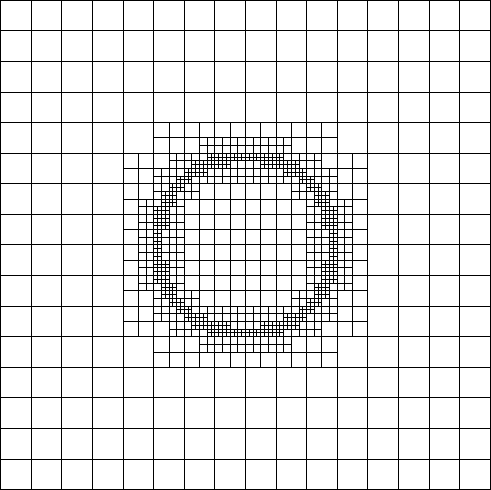 Figure 1
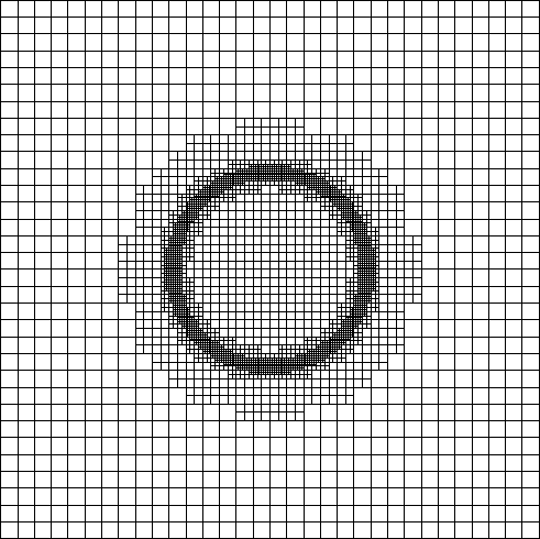 Figure 2
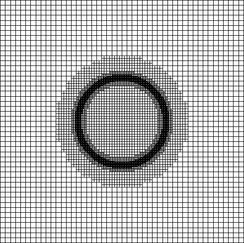 Figure 3
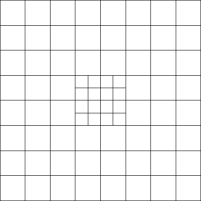 Figure 4
 Figure 5
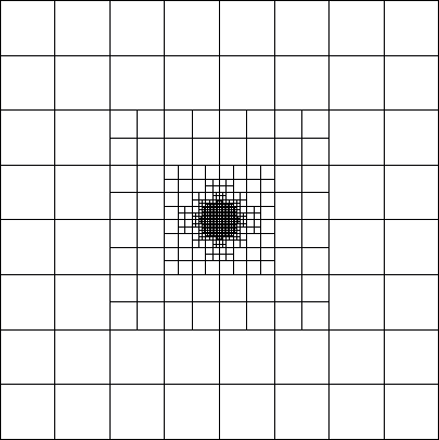 Figure 6
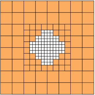 Figure 7
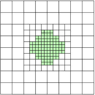 Figure 8
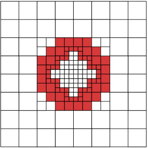 Figure 9
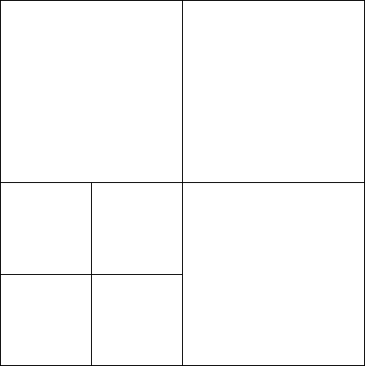 Figure 10
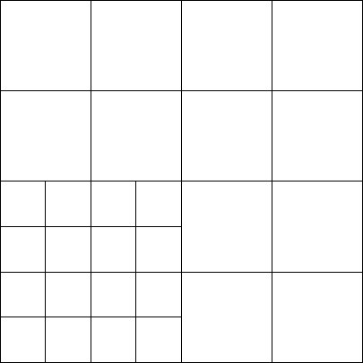 Figure 11
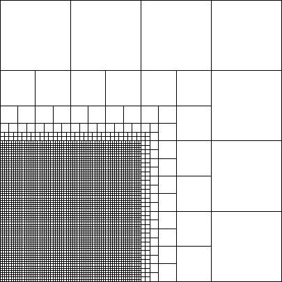 Figure 12
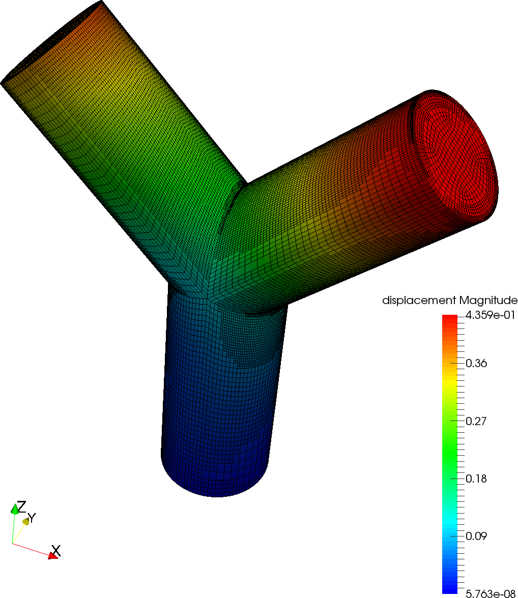 Figure 13
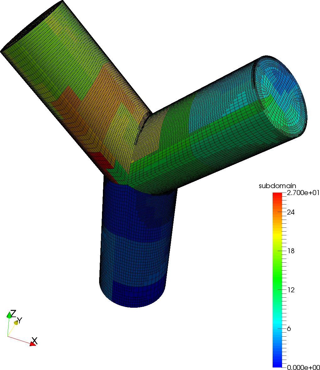 Figure 14
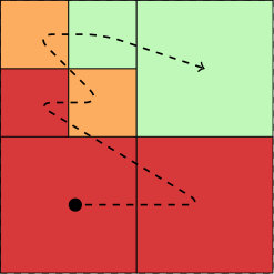 Figure 15
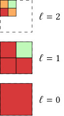 Figure 16
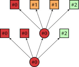 Figure 17
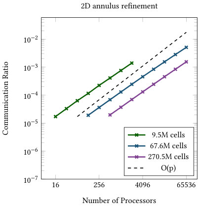 Figure 18
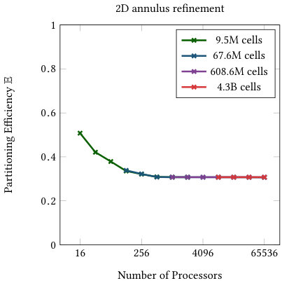 Figure 19
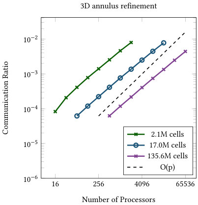 Figure 20
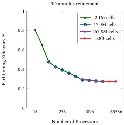 Figure 21
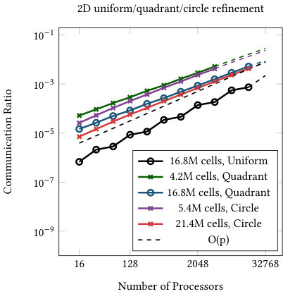 Figure 22
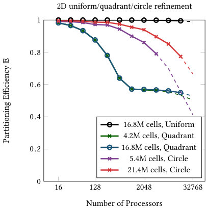 Figure 23
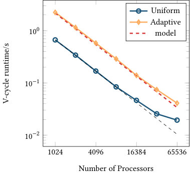 Figure 24
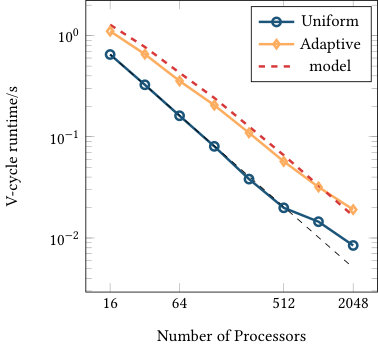 Figure 25
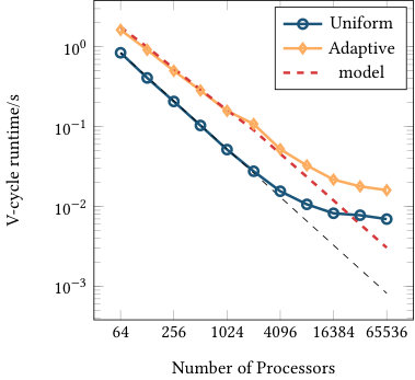 Figure 26
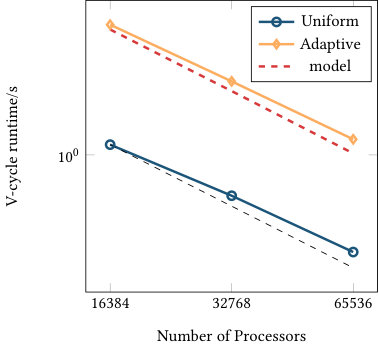 Figure 27
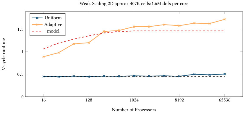 Figure 28
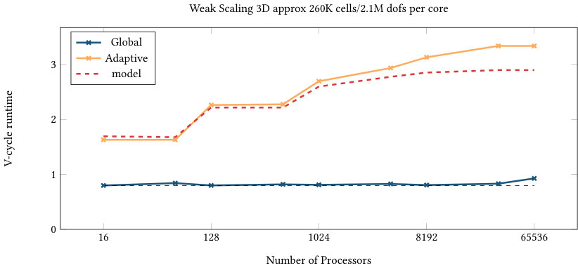 Figure 29
| Partition efficiency | Communication ratio | |||||||
|---|---|---|---|---|---|---|---|---|
| level | cells | ghost | native | ratio | ||||
| 0 | 125 | 1 | 1 | 0.1221 | 0.12207 | 513 | 487 | 0.51300 |
| 1 | 1,000 | 8 | 1 | 0.9766 | 0.12207 | 866 | 7,134 | 0.10825 |
| 2 | 8,000 | 64 | 8 | 7.8125 | 0.12207 | 2,028 | 61,972 | 0.03169 |
| 3 | 64,000 | 506 | 63 | 62.500 | 0.12352 | 3,118 | 508,882 | 0.00609 |
| 4 | 512,000 | 4,048 | 500 | 500.00 | 0.12352 | 3,017 | 354,743 | 0.00843 |
| 5 | 357,760 | 3,988 | 350 | 349.38 | 0.08761 | 2,635 | 807,349 | 0.00325 |
| 6 | 809,984 | 2,316 | 791 | 791.00 | 0.34154 | 0 | 2,977,280 | 0.00000 |
| 7 | 2,977,280 | 4,048 | 2,908 | 2,907.5 | 0.71826 | - | - | - |
| Total | 4,730,149 | 14,979 | 4,622 | 4,619.3 | 0.30838 | 12,177 | 4,717,847 | 0.00257 |
| coarse direct solver | coarse CG/AMG iteration | |||||||
| time | time / DoF | coarse solve | time | time / DoF | ||||
| levels | DoFs | CG its | [s] | [s / DoF] | CG its | avg CG its | [s] | [s / DoF] |
| 2 | 1,819,584 | 27 | 46.1 | 25.3 | 27 | 28.8 | 113.4 | 62.3 |
| 3 | 2,456,325 | 27 | 63.6 | 25.9 | 27 | 29.7 | 152.7 | 62.2 |
| 4 | 4,916,538 | 28 | 121.7 | 24.8 | 28 | 29.7 | 251.9 | 51.2 |
| 5 | 11,684,817 | 28 | 260.3 | 22.3 | 28 | 27.8 | 420.0 | 35.9 |
| 1 node | 4 nodes | 16 nodes | 64 nodes | ||||||
| without | without | without | without | ||||||
| levels | DoFs | time | coarse | time | coarse | time | coarse | time | coarse |
| 2 | 1.8M | 27.3 | 14.9 | 35.5 | 5.2 | 30.3 | 1.5 | 40.9 | 0.4 |
| 3 | 2.5M | 44.5 | 28.7 | 32.7 | 8.4 | 30.5 | 3.0 | 30.1 | 1.1 |
| 4 | 4.9M | 85.9 | 71.5 | 51.2 | 21.4 | 34.9 | 7.8 | 45.8 | 2.8 |
| 5 | 11.7M | 188.3 | 173.1 | 82.7 | 54.4 | 48.9 | 18.2 | 35.1 | 6.3 |
| 6 | 35.7M | — | — | 212.1 | 185.3 | 91.3 | 62.1 | 48.8 | 20.6 |
| 7 | 101.1M | — | — | — | — | 214.2 | 178.9 | 92.8 | 61.6 |
| 8 | 316.8M | — | — | — | — | — | — | 262.3 | 227.8 |
| Setup | total | |||||||||
| Proc | Cycle | DoFs | mesh | FE | assembly | prec | total | solve | time | |
| MF | 112 | 13 | 4.1M | 0.562 | 0.151 | 0.029 | 0.393 | 1.135 | 0.200 | 1.335 |
| 448 | 15 | 16.3M | 0.703 | 0.154 | 0.027 | 0.535 | 1.419 | 0.253 | 1.672 | |
| 1792 | 17 | 65.1M | 0.910 | 0.182 | 0.030 | 0.686 | 1.808 | 0.309 | 2.117 | |
| 7168 | 19 | 256.3M | 1.030 | 0.152 | 0.032 | 0.893 | 2.107 | 0.521 | 2.628 | |
| MB | 112 | 13 | 4.1M | 0.564 | 0.527 | 0.623 | 2.934 | 4.648 | 0.716 | 5.364 |
| 448 | 15 | 16.3M | 0.702 | 0.548 | 0.677 | 3.776 | 5.703 | 1.190 | 6.893 | |
| 1792 | 17 | 65.1M | 0.898 | 0.575 | 0.698 | 4.862 | 7.033 | 1.660 | 8.693 | |
| 7168 | 19 | 256.3M | 1.040 | 0.619 | 0.727 | 7.260 | 9.646 | 2.560 | 12.206 | |
| AMG | 112 | 13 | 4.1M | 0.296 | 0.507 | 0.657 | 0.405 | 1.865 | 0.924 | 2.789 |
| 448 | 15 | 16.3M | 0.339 | 0.534 | 0.671 | 0.456 | 2.000 | 1.150 | 3.150 | |
| 1792 | 17 | 65.1M | 0.421 | 0.553 | 0.680 | 0.546 | 2.200 | 1.460 | 3.660 | |
| 7168 | 19 | 256.3M | 0.515 | 0.585 | 0.744 | 1.010 | 2.854 | 1.890 | 4.744 | |
Peer Reviews
No public reviews on file for this paper yet. If you reviewed it on a platform where reviews are public (OpenReview, ICLR, NeurIPS, ICML), you can paste yours below so the community can read it here.
Code & Models
Videos
No videos yet. Explain this paper in a talk, walkthrough, or lecture? Add one.
A Flexible, Parallel, Adaptive Geometric Multigrid Method for FEM
Thomas C. Clevenger
[email protected], Clemson University
,
Timo Heister
[email protected], Clemson University
,
Guido Kanschat
[email protected], Heidelberg University
and
Martin Kronbichler
[email protected], Technical University of Munich
Abstract.
Note: This is a preprint of the published article in ACM TOMS, see https://doi.org/10.1145/3425193.
We present the design and implementation details of a geometric multigrid method on adaptively refined meshes for massively parallel computations. The method uses local smoothing on the refined part of the mesh. Partitioning is achieved by using a space filling curve for the leaf mesh and distributing ancestors in the hierarchy based on the leaves. We present a model of the efficiency of mesh hierarchy distribution and compare its predictions to runtime measurements. The algorithm is implemented as part of the deal.II finite element library and as such available to the public.
Key words and phrases:
multigrid, message passing, finite element methods
1. Introduction
Geometric multigrid methods are known to be solvers for elliptic partial differential equations with optimal complexity in the number of total variables [31, 22], but optimal performance in a massively parallel environment depends on more than complexity alone. Sufficiently many concurrent operations must allow utilization of a sufficiently large part of the system, and it is not clear a priori if multigrid methods with their hierarchy of coarse meshes and synchronization due to grid transfer will be efficient on such systems. In this article, we present algorithms for such a method and demonstrate its feasibility in experiments.
Geometric multigrid methods for adaptive meshes and their implementation on parallel computers have been studied for almost four decades, for instance by [51, 13, 15] and others. A breakthrough was obtained in the late 1990s by the use of space filling curves (see [52] and literature cited therein), which allow the partitioning of a hierarchical mesh in almost no time. Thus, load balancing was reduced from an np-hard problem to a negligible task. Such methods were implemented for instance in the software libraries p4est [25], deal.II [11], DUNE [16], and Peano [50, 49].
Several different kinds of adaptive multigrid methods can be distinguished from the types of meshes and level spaces. Meshes can either be conforming or nonconforming. Conforming meshes are generated by bisection, or by refinement into children in dimensions dividing all edges and subsequent closure (red-green refinement). These methods are most commonly used with simplicial meshes, and typically require mixed topologies otherwise. The alternative are nonconforming methods, most prominently the one-irregular meshes introduced by Bank, Sherman, and Weiser [14]. Here, the difference in refinement between two cells sharing a common edge may not exceed one level. This constraint is not necessary and there have been codes which allow arbitrarily different refinement levels of neighbors (see [8] and references therein). It nevertheless simplifies the code considerably in particular in view of modern architectures. This method has been implemented for simplicial meshes as well as meshes based on (deformed) hypercubes. Since the meshes are nonconforming, additional care has to be taken to ensure conformity of associated finite element spaces. This is achieved by “elimination of hanging nodes” resulting in algebraic constraints on the possible finite element functions on the finer cell, see for instance [51].
After a locally refined mesh has been constructed, typically in an adaptive algorithm, and its finite element space has been properly defined with or without “hanging nodes”, the resulting mesh has cells on different levels. Thus, using a multigrid algorithm employing smoothing operations on all cells on “level or less” is not of optimal complexity on arbitrary meshes. Two remedies have been proposed: local smoothing [23, 35, 34, 2] and global coarsening [44, 19, 46]. We apply the former approach in this work. While optimal parallel work balance is more of a challenge with local smoothing, there are a few potential advantages over global coarsening that justify the investigation in this paper. First, the computational complexity for the former is slightly lower and optimal on all meshes, while there are (extreme) examples for suboptimal complexity of global coarsening. Second, the smoothing operation is always run on meshes without hanging nodes; while this is not an issue for point smoothers like the Jacobi method, it facilitates block smoothers, in particular patch smoothers as in [7, 36]. Finally, implementation on vectorizing and multicore architectures is fairly straight-forward and does not require special care at hanging nodes.
The hardware properties of state-of-the-art supercomputers have evolved most rapidly in terms of the node-level performance in the last decade, whereas network topologies across the nodes and node numbers have been relatively steady with a thousand to ten thousand nodes on the top machines. For these reasons, algorithmic components and data structures that have low communication requirements are essential to balance inter-node latencies with increasing intra-node performance, which can rely on hybrid parallelism, matrix-free algorithms to relax the memory bandwidth requirements [18, 17, 42, 40], as well as wide vectorization or offloading to GPUs, see e.g. [41] and references therein. These node-level optimizations provide fast matrix-vector products for use in smoothers and level transfer, including nearest-neighbor communication in the network. The main focus of the present work is on the algorithmic framework of local smoothing multigrid targeting the inter-node case of large-scale parallel computations with MPI on meshes with adaptive refinement. The components are flexible and allow for an arbitrary element degree, various conforming or non-conforming elements, as well as systems of equations, extending previous work on massively parallel multigrid [43, 3, 47, 45, 27]. Our contribution is integrated into the deal.II finite element library and available as open-source software [4, 5].
Our approach shown here can be summarized as a geometric multigrid method on adaptively refined meshes. Each V-cycle is built from smoother, transfer, and coarse solver operators that are equivalent to the serial method, while the work and data structures are distributed in parallel. In practice, it is common to use Krylov methods, like conjugate gradient, and perform a multigrid cycle as a preconditioner instead of using multigrid as the solver. This is the approach we use in the numerical examples.
The remainder of this work is structured as follows. In §2, we present the geometric multigrid algorithm based on local smoothing. The components for parallel execution in terms of the mesh infrastructure, supported by an efficiency analysis of one particular partitioning strategy, are given in §3. Performance results are shown in § 4 and the work is concluded in § 5.
2. Geometric multigrid with local smoothing
2.1. Bilinear forms and finite element discretization
The basis for our method is a partial differential equation in weak form, abstractly written as: find such that
[TABLE]
Here, is a suitable solution space and . For example, the Poisson equation with homogeneous Dirichlet boundary condition on the domain and right hand side translates to and the weak equation
[TABLE]
Our second example are the Lamé–Navier equations of linear elasticity in space dimension , where . With the strain operator , we obtain
[TABLE]
These weak forms are discretized by the finite element method. To this end, we introduce a mesh covering the domain . This article describes functionality of the library deal.II, see [4], where the mesh cells are quadrilaterals and hexahedra in two and three space dimensions, respectively. We use mapped elements and the mappings from the reference cell to the actual grid cell is not restricted to -linear functions or polynomials, but can be any function. On each mesh cell, we define a local shape function space, typically by mapping polynomials defined by a set of interpolation points from the reference cell . Using degrees of freedom, we establish continuity between cells and define a basis of the finite element space on the mesh . In the conforming case, the finite element discretization of equation (1) becomes: find such that
[TABLE]
We will not distinguish between finite element functions and their coefficient vectors with , since the meaning will be clear from context. The basis used for this identification consists of standard nodal finite element functions with local support.
Discontinuous Galerkin (DG) finite element methods are an alternative to conforming methods. Starting with the same mesh, we introduce finite element spaces which are no longer conforming to the space , i.e. , in particular spaces with no continuity requirements. Therefore, the straight-forward discretization using (4) is inconsistent and typically not converging to the continuous solution. This is remedied by introducing so-called flux terms on the interfaces, which guarantee consistency and stability of the method. Accordingly, the bilinear form on depends on the mesh itself and we write: find such that
[TABLE]
As an example, we mention the interior penalty method [6] for the Laplacian with its multilevel analysis in [28] and the bilinear form
[TABLE]
The right-hand side with Dirichlet boundary data is
[TABLE]
Here, are the -dimensional interfaces between mesh cells of and are the facets of cells on the boundary of . Every face has two adjacent cells, say and . We call the restriction of the finite element functions and to these cells , , , and , respectively. With these definitions, we have the jump and mean value operators
[TABLE]
Finally, is an appropriately chosen penalty parameter inversely proportional to the diameter of the cells attached to the face .
2.2. Geometric multigrid
The geometric multigrid method employs a hierarchy of meshes, which we generate as follows. Starting from the coarse mesh , we generate the mesh from by selecting a subset or all of its cells and refining these isotropically by bisecting each edge, generating children each. This results in a sequence
[TABLE]
where the symbol “” denotes nested meshes, that is, every cell of a mesh on the left of this symbol is the union of one or more cells of the mesh on the right.
As usual, we define finite element spaces on these meshes by defining local shape function spaces on each cell and concatenating these spaces, identifying shape functions on adjacent cells which are associated to joint degrees of freedom. For most finite elements, and these are the ones we consider here, the shape functions on a cell can be represented as linear combinations of the shape functions on its children in the mesh hierarchy. Therefore, the mesh hierarchy above induces a sequence of finite element spaces
[TABLE]
We discretize the weak formulation (1) on each mesh by a bilinear form and the problem: find , such that
[TABLE]
For conforming finite element methods, the bilinear forms and the right hand side are simply the restrictions of and to the space . For DG and other stabilized schemes, they contain additional terms for consistency and stability. Associated with the bilinear form is a linear operator defined by
[TABLE]
Here, the inner product on is the one used in the conjugate gradient method, typically the Euclidean norm of the coefficient vector of a function with respect to the nodal basis of , see for instance the discussion of mesh dependent norms in [21, 24] and their relation to the inner product of . Based on the embeddings in (10), we define the grid transfer operators
[TABLE]
On each mesh level , we employ a smoother , which employs the right hand side and the current state to compute a result. Examples for such smoothers are relaxation methods of the form in Algorithm 1.
Here, is the number of smoothing steps and is the type of relaxation method, for instance the diagonal for the Jacobi method or the lower triangle for Gauss–Seidel. Similarly, additive and multiplicative Schwarz methods fit into this concept, but it also extends to nonlinear methods like conjugate gradients or GMRES.
We are now ready to state the multigrid V-cycle algorithm in Algorithm 2 in abstract form, as it has been done in numerous publications. In addition to the level transfers and smoothers discussed before, the recursion of the algorithm requires closure at level 0, denoted as the inverse of . This is called coarse grid solver, and in an implementation can be a direct solver since the system is small, or a basic iterative method like conjugate gradients or GMRES since the system is well conditioned.
2.3. Level meshes and local smoothing
For uniformly refined meshes, the definition of the level meshes is trivial. For adaptively refined meshes, we consider the hierarchy as a tree or a forest (for more than one coarse cell). Each node of this forest is a cell in the mesh hierarchy. The cells of the coarse mesh are the roots of its trees. The level of a cell is defined as the distance from its root. The mesh on which we discretize the differential equation consists of the leaves of this tree (or forest) and is denoted as the leaf mesh . Since it is obtained by local refinement, it typically consists of cells on different levels up to level .
For intermediate levels , two different schemes have been devised. First, for global coarsening, the meshes are constructed from the leaf mesh. The mesh is obtained by replacing all cells in by their immediate parents in the forest. Once a cell of the coarse mesh is reached, it remains in further level meshes. For more information we refer to [19, 46].
Instead, in our definition of the level mesh consists of all cells of level and of all leaves with level less than . With such a definition of , a fairly coarse leaf cell can be part of many different level meshes.
In order to obtain an algorithm with optimal complexity, smoothing for the degrees of freedom of a given cell should only happen on a single level. This is where local smoothing enters: while we are running a multigrid method for the whole finite element space , we restrict smoothing only to the mesh cells which are actually on level . This splitting is explained in Figure 1.
The mesh is split into the submesh of cells strictly on level and of cells on lower levels than . For DG methods, this immediately results in a splitting , where the support of each subspace is its corresponding submesh. The splitting for continuous methods is more complicated since there are finite element basis functions with support straddling the interface and thus in both and . The span of these basis functions is called , the space of interface functions.
We now give a short review of the structure of the operators in the multigrid method outlined in [35, 34]. Here, the goal is to implement the algebraic equivalent of the original multigrid method for the space hierarchy with operators obeying the subspace splitting. We start with the observation that conforming methods require the function on the refined side of a refinement edge to coincide with the function on the coarse side. This translates into elimination of degrees of freedom on the refined side such that uses degrees of freedom representable on the coarse mesh only. The fact that shape functions in have different support from their counterparts in is taken care of by the grid transfer operators.
Thus, we can restrict smoothing on level to and can ignore . Furthermore, in the case of DG methods, , such that in both cases we can write . Our assumptions on local smoothing translate to
[TABLE]
where is now the local smoother on only. We observe that the embedding operator maps a function from to itself. Therefore, is the identity on . Thus, has the structure
[TABLE]
Note that the restriction operator involves more than two levels if its range is not in , because the other components of are not stored on this level. Therefore, we simplify the code considerably if we ensure . This can be achieved by an additional mesh refinement rule: require that there is a complete layer of cells on level surrounding .
Residuals on the other hand must be computed correctly on the whole space according to
[TABLE]
Note that the matrices and are the flux matrices of a DG method on the refinement edge and thus vanish for conforming methods. Furthermore, we see in the V-cycle algorithm that this residual is immediately restricted to the coarse space . Since the restriction acts as identity on , we can avoid computing and defer it to the lower level. Thus, the matrix is not needed in computations at all. The matrix is used for smoothing on level . The off-diagonal matrices correspond to coupling between degrees of freedom on the cells at the interface, and are needed in addition to for a consistent multigrid method.
A major advantage of local smoothing is its fairly simple data structure. The level meshes do not have hanging nodes, such that the results of cell-wise operations can be entered into global vectors very efficiently without any elimination process. This also simplifies implementation, especially when considering more involved smoothers such as patch smoothers, that would need to operate on patches of cells on different refinement levels. Furthermore, it is of optimal computational complexity on any locally refined mesh, while global coarsening may be suboptimal on some meshes with extreme local refinement, see [34]. Nevertheless, this second aspect does not seem to have much impact on actual computations.
3. Parallelization of geometric multigrid
We will now discuss the construction of an efficient and scalable parallel version of the adaptive multigrid method described in Section 2. We emphasize data and communication structures while keeping the algorithm mathematically equivalent to the weathered sequential version. Regarding parallelism, we have to consider three levels of parallelization in modern computer architectures, namely message passing between computer nodes and intra-node parallelization separated in multicore/multitasking (multiple instruction, multiple data) and vectorization (single instruction, multiple data). As motivated in the introduction, this article focuses on message passing. The intra-node parallelization approach employed is shortly discussed in §3.2.
A scalable approach requires distributed data structures and scalable algorithms operating on them including equal partitioning of the work. As demonstrated in the computations in the later sections of this paper, the parallel algorithms described here enable high resolution adaptive computations with billions of unknowns on 100,000+ cores. We concentrate on MPI as the parallelization framework and we refer to a single MPI rank or process as “processor”.
3.1. Parallel algorithm
Our algorithm is synchronized between applications of residual, smoothing, grid transfer operators, and coarse grid solvers. Hence, our focus lies in the parallel implementation of these operators.
The abstraction of parallel data structures and algorithms equivalent to the serial version is well-known. Libraries such as PETSc [9, 10] and Trilinos [33] have provided linear algebra data structures (vectors, sparse matrices) and algorithms (iterative solvers) with this abstraction for a long time. Up to a point, this isolates the user (for example finite element library implementors) from having to interface directly with the underlying parallel computing framework. Abstraction of this kind are of course not perfect, because operations like finite element assembly need to be partitioned between the processors. Nevertheless, it enables the design of parallel algorithms on a higher level, like it is done in deal.II, see [11].
The workload is typically distributed by partitioning the cells of the computation using graph based partitioners or using space-filling curves (like METIS [38], Zoltan [20], or p4est [25] – the latter one being used in deal.II). This partitioning can be used to distribute cell-based work, like matrix or residual assembly, and can be used to generate a partitioning of degrees of freedom that is needed for the row-wise division of linear algebra objects (vectors, matrices). The latter step requires a rule to decide on the ownership of degrees of freedom on the interface between processor boundaries of the cells. For the finite element framework, the main effort is to correctly assign and communicate ghost cells and ghost indices, while the communication for matrix-vector products and finite element assembly of foreign entities only involves neighboring processors and is typically provided by the linear algebra libraries.
Here, we will follow the same approach for the partitioning of cells and degrees of freedom on each level of the multigrid hierarchy: after partitioning of all cells strictly on level in some way, we use this to partition the degrees of freedom accordingly. Like above, it is advantageous for large computations if only part of the mesh that is relevant for the current processor are stored locally. There are different options for partitioning cells on each multigrid level. We will discuss different strategies and the approach we take in Section 3.3, but stress that our implementation is flexible in this respect.
While knowledge about the whole mesh is not required, we need ghost neighbors on each level, which can be on different levels in adaptive computations. In our implementation, we decided to always construct the ghost neighbors as the set of all cells that share at least a vertex with the local cells and exchange all information about them, even though specific implementations might require less information (for example only neighbors across faces for DG). Furthermore, information about parents/siblings is required for transfer operations. This allows us to compute and exchange the necessary information about degrees of freedom for smoothing and grid transfer.
To summarize the execution of multigrid in parallel, the following parallel ingredients are necessary:
- •
Prolongation and restriction are conceptually a multiplication of distributed vectors with a rectangular transfer matrix and as such equivalent to the serial transfer. Known algorithms for sparse matrix-vector products scale well in parallel.
- •
The smoothers we consider are conceptually a sequence of local operations on individual degrees of freedom or small subspaces. Additive smoothers (Jacobi, additive Schwarz, etc.) can be run in parallel on all processors and are still equivalent to the serial method. Sequential smoothers (Gauss–Seidel, multiplicative Schwarz, etc.) can of course not be used immediately.
Other parallelizable smoothers (for example block Gauss–Seidel variants) may not be equivalent to their sequential version. Only in this case equivalence to the sequential multigrid algorithm is lost, which can lead to an increase in iteration numbers when increasing the number of processors, albeit they often remain more effective than additive smoothers.
- •
There are several options for coarse solvers. First, if the problem is reduced to a very small number of cells and processors, runtime is negligible and (parallel) direct solvers can be applied. In other cases, when the coarse mesh still has a large number of degrees of freedom, switching to algebraic multigrid is an option used in [46, 47] for example and what we use in Section 4.2.
3.2. Matrix-free implementation
In the previous sections, we have derived the multigrid algorithm in an abstract way based on linear algebra operators. While these are typically implemented as sparse matrices, the concept directly translates to matrix-free operator evaluation. These methods often provide considerably faster evaluation of matrix-vector products than assembled matrices, in particular for higher order finite elements, because the access to memory is significantly reduced [39, 40], which is the limiting factor in matrix-based implementations. In this work, we consider methods based on sum factorization techniques on hexahedra which have a particularly high node-level performance [42] and are also applicable to GPUs [41]. We note that a fast intra-node performance puts more emphasis on possible communication bottlenecks.
3.3. Partitioning strategy for mesh hierarchy
When partitioning the cells on each level of the multigrid hierarchy, a balance between several conflicting goals is necessary:
- (1)
Minimize communication for transfer operations between multigrid levels. 2. (2)
Fair work balance on each level (same number of cells per processor). 3. (3)
Minimize interface between processor boundaries on each level (minimizes communication in smoother applications or residual computations). 4. (4)
Minimize required additional storage for the mesh hierarchy if local cells have little overlap between levels.
Previous work [46] has concentrated mainly on aspect (2) by using an independent partition on each level. The multigrid method there is based on global coarsening instead of local smoothing, so each level is an adaptively refined mesh that needs to be partitioned. While satisfying (2), this ignores (1) and requires duplicate storage, violating (4). Experiments in [46] have shown excellent scaling despite these deficiencies. Note that (1) is satisfied for meshes refined mostly globally, but duplicate storage (4) is still required. It is worth pointing out that the storage requirement reduces by a factor of 8 in each coarsening step in 3d.
In this work, we explore algorithms that ignore (2) and partition the hierarchy based on the partitioning of the leaf mesh to minimize communication cost and storage requirements (goal (1) and (4)). This option also represents a straight-forward implementation in terms of local tree data structures and can be seen as a baseline to more sophisticated setups. We will see that we satisfy goal (2) for mostly globally refined meshes and that we can quantify the partitioning efficiency (see Section 3.4).
Note that both approaches behave similarly for uniformly refined meshes, while goals (1) and (2) are conflicting for an adaptive scheme. Finally, note that (2) is desired when assuming that levels are passed through sequentially, as the multigrid algorithm suggests, but one could design a parallel method that does not require synchronization on each level.
In the following, we will partition the multigrid cells by the “first-child rule” as follows: First, distribute the leaf cells using a space filling curve (we use p4est [25] as described in [11]). Second, for each cell in the hierarchy, recursively assign the parent of a cell to the owner of the first child cell. A similar strategy has been used also by the Octor package [48] for the parent-child relationships.
For an example with seven cells, see Figure 2 that shows the mesh with the space-filling curve on the left, the tree representing the refinement in the middle, and the cells on each level on the right. This approach has the following consequences:
- (1)
The local cells and their parents are already present on each processor and the ownership of parents is known without any communication. This means the partitioning of the multigrid hierarchy can be done without communication. 2. (2)
No duplicated storage for the mesh is needed as all parent cells are already stored locally (goal (4)). 3. (3)
Transfer operations are local and require only a small amount of communication at processor boundaries (goal (1)). 4. (4)
Processors drop out automatically on coarser levels, which is desired. 5. (5)
The workload on each level is not distributed equally.
We will discuss the last point and its impact in the next subsection.
3.4. Partitioning efficiency model
Our model for the complexity of the partitioned workload, in short parallel complexity, is based on the assumption that parallelization is completely achieved by MPI ranks and that within each rank the workload is proportional to the number of cells. Below, we develop a complexity model based on this assumption, estimating the parallel complexity of our algorithm in terms of mesh cells per level.
Let be the number of cells on level and of the subset owned by processor . Here, cell refers to all cells in the hierarchy, not only leaf cells belonging to the discretization mesh. We assume that the workload for each cell is equal, such that is proportional to the total amount of work a processor has to invest on level . Obviously, the optimal parallel complexity is
[TABLE]
Here, the terms in brackets specify the total work of the multigrid algorithm and the total number of processors is given by . is the cost of the coarse grid solver, which may be different than the cost of a smoother application.
This calculation is based on perfect equidistribution of work and neglects communication overhead. In particular, it is not achievable if grid transfers are synchronized, as in our implementation. In this case, we can only distribute the work on each level such that we are bound from below on each level by
[TABLE]
where is the smallest integer greater or equal to . Therefore, the best achievable work time with syncing between levels is
[TABLE]
On the other hand, with imperfect distribution of work, the limiting effort on each level is
[TABLE]
and the total parallel complexity and partitioning efficiency due to imbalance against a hypothetical optimal partitioning are given by
[TABLE]
To summarize, the efficiency quantifies the overhead produced by not having a perfect work balance on each level of the multigrid hierarchy. The work is modeled as one unit per cell and, as such, can be used to model the computational cost for grid transfer, smoother application, and other operations. The efficiency, by definition, accumulates the imbalances on each level.
We give an example for these estimates for the mesh hierarchy displayed in Figure 2. It consists of 7 leaf cells obtained by successive refinement of a single coarse cell. The partitioning is done for three processors. The ownership of the leaf cells is determined by p4est using a space-filling curve (-curve, also known as Morton curve, dashed line on the left picture) or depth-first traversal (from left to right) in the tree representation depicted in the middle. The ownership of cells in the multigrid hierarchy (round circles in the tree) is determined by copying the leaf ownership and then applying the “first-child rule” recursively. For example, the parent of the four smallest cells on level 2 is red (#0) because the first (bottom-left) child also belongs to processor #0 (red).
One result of this partitioning is that processors drop out on coarser levels automatically. Here, processor #1 (green) recuses itself on level 1 and only processor #0 (red) remains on the coarsest level (here a single cell). The coarsest mesh is not necessarily completely owned by processor #0 if it consists of more than a single cell.
The optimal parallel complexity is simply the number of all cells in the hierarchy divided by the number of processors, hence . On the other hand, assuming the coarse grid solver has the same complexity as the work load per cell on higher levels,
[TABLE]
Comparing to
[TABLE]
we obtain in this example. In other words, our model predicts a slowdown of 100% and 20% compared to and , respectively. The slowdown with respect to is due to the non-optimal partitioning on level 1, where processor # 0 (red) works on three cells while the other processors have to wait. An optimal partitioning would only require operating on two cells sequentially on that level. Compared to , we do not have enough cells to keep three processors busy.
This example suggests that the efficiency of the algorithm depends significantly on the base of comparison, or . In fact, a closer inspection of the definitions reveals that they only differ by rounding up the load on each level to the next multiple of , a difference which drops below 1% as soon as we have 100 cells on each processor. Below, we only use when we assess the efficiency of our mesh hierarchy distribution.
3.5. Experimental study of the efficiency of the first-child rule
Making general conclusions about the partitioning efficiency is difficult as it depends on the number of processors, the coarse mesh, and the refinement. Instead, we study the efficiency for several test cases shown in Figure 3.
These are obtained by the following construction. All are based on a coarse mesh consisting of a single cell defined by . Finer meshes, where denotes the level of the finest cells, are obtained recursively by one of the following selection criteria:
**“uniform”: **
global refinement of the coarse mesh times, obtaining a uniform leaf mesh of cells in two dimensions.
**“circle”: **
times refinement of all mesh cells with at least one vertex inside the circle of radius around the origin.
**“quadrant”: **
times refinement of all mesh cells in the negative quadrant.
**“sine curve”: **
times refinement of all mesh cells intersected by the curve (plane for 3d) .
**“annulus”: **
After uniform refinements, add the steps:
- **(1): **
Refine all cells whose center lies in the circle (sphere for 3D) of radius . 2. **(2): **
Refine all cells in the shell between radius and . 3. **(3): **
Refine all cells in the shell between radius and .
All these procedures are completed by a closure after each refinement step, ensuring one-irregularity in the sense that two leaf cells may only differ by one level, if they share a degree of freedom or a face for conforming methods and for DG methods, respectively. These conditions are imposed in the deal.II library for practical reasons, because they simplify several aspects of the implementation. They can be relaxed at the price of software complexity.
Figure 4 shows the partitioning efficiency as defined in (18) for varying processor count and problem size. For uniformly refined meshes we observe 100% efficiency (this also holds in 3d, not shown). This is due to the fact that processor counts are multiples of , which implies perfect partitioning on each level. The “quadrant”, “sine curve”, and “annulus” refinement schemes show roughly the same behavior. Their efficiency drops until it levels off at 60% for the quadrant and 2d sine curve, 50% for the 3d sine plane, and about 30% for the annulus in two and three dimensions. This level of efficiency is then maintained over a wide range of processor counts. It only begins dropping again when the problem size is down to less than 1000 cells per processor, especially for the “circle” and ”sine curve” refinements. Both are extreme cases with very localized refinement and these examples have fewer cells compared to many of the other examples. For realistic problem sizes (more than 1000 active cells per processor), their efficiency remains above 50%.
All of this information together suggests that, given a sufficient number of cells per processor, the imbalance of this distribution is primarily dependent on the type of mesh refinement refinement scheme. The number of processors influences the efficiency only to a certain “leveling off” point. In all cases, the efficiency stays above 30% compared to the optimal workload. In order to reach higher efficiency, re-partitioning and additional communication to processes farther away would be necessary.
Table 1 gives a level-by-level breakdown of the partition efficiency for the 3D annulus refinement with 4.1M cells on 1,024 processors. Predictably, the efficiency is very low at lower levels where there are fewer cells, and trends towards 1 for higher levels. It should be noted that the partition efficiency calculated using would be very different on lower levels than the value in the table which uses (this is seen on the smaller example in Section 3.4). However, the difference in the total efficiency over all levels is only around 0.1% with a value of 0.309 using as compared to 0.308 using .
3.6. Communication
The second factor determining the performance of parallel algorithms, next to load balancing discussed above, is communication overhead. Communication is not only much slower than computation at the granularity of individual instructions, it also consumes more energy, because electrical charges must be transported over fairly long distances. We introduced the first-child rule with the express purpose to reduce communication overhead and keep it small compared to the local computations. In this section, we set out to demonstrate that this goal was achieved.
Communication happens in matrix-vector products and in grid transfer operations. Both of them apply a linear operator to a global discretization vector. The communication overhead in the first case is reduced by partitioning the leaf mesh into subdomains, such that their surface per volume ratio is small. Since the surface is of lower dimension, this implies that communication cost tends to zero as the number of cells on each processor grows to infinity. For weak scaling, this implies that it remains small compared to local operations, as long as there are sufficiently many cells on each processor. Such a partitioning is efficiently achieved by a space filling curve, in our case, the -curve. Enumerating the cells along such a curve implies that cells with close indices will typically be close geometrically. This approach has been a standard for many years now.
The first child rule for partitioning lower levels achieves a similar goal for grid transfer operations. If most children are on the same processor as their parents, the amount of communicated data is also much lower than the total amount of data processed. In Figure 5, we show that the number of “ghost children” is indeed very small compared to the total number of children. And while these numbers are rising with the number of processors, in the worst case observed less than 1% of the cells require communication. Additionally, the total communication volume seems to grow more slowly than the number of processors involved in the communication.
Finally, Table 1 gives a level-by-level breakdown of the communication ratio for the 3D annulus refinement with 4.1M cells on 1,024 processors. Each of the higher levels require the communication of about 2,000-3,000 cell during the transfer, with the exception of the highest level, which requires no communication since the p4est distribution used for the active level requires that all groups of terminal children are owned by the same processor. For refinement schemes where the majority of active cells are of the highest refinement level, this will result in low communication ratios, as is seen with global refinement in Figure 5.
4. Performance Results
The algorithm described in the previous sections has been implemented in the deal.II finite element library [12, 4]. The partitioning of the adaptively refined meshes uses p4est [25]. The implementation with sparse matrices uses Trilinos EPetra [33], while the matrix-free implementation is based on data distribution algorithms built into deal.II. The source code and parameters of the examples in this manuscript are available at https://github.com/tjhei/paper-parallel-gmg-data.
4.1. Scaling on SuperMUC
As a first experiment, we consider the constant-coefficient Laplacian on a cube, discretized with elements, and compare the runtime on a uniform mesh against an adaptively refined case with the annulus refinement. The adaptive mesh is set up such that the number of cells matches with the number of cells in the uniform case within 2%. The computations are run on phase 1 of SuperMUC, providing nodes with cores of Intel Xeon E5-2680 (Sandy Bridge), connected via an Infiniband FDR10 fabric. For pre- and post-smoothing, a Chebyshev iteration of the Jacobi method with Chebyshev degree five, i.e., five matrix-vector products, is selected [1]. The relatively high degree of the Chebyshev smoother is the result of an experimental study for the best run time for the chosen implementation described below on uniform grids. Most important to the decision is the mixed-precision setup with smoothing done in single precision as described in [41, 26]. The parameters of the Chebyshev polynomial are set to damp contributions in the eigenvalue range on each level . The estimate of the largest eigenvalue of the matrix is computed by a conjugate gradient iteration with 10 iterations from an initial vector of zero mean constructed as . As a coarse solver, the Chebyshev iteration is selected with a degree chosen such that a priori error estimate of the Chebyshev iteration ensures a residual reduction by , now for the full eigenvalue range of the coarse level matrix determined by a conjugate gradient solution to a relative tolerance in the unpreconditioned residual of . The coarse grid tolerance is chosen as a balance between the accuracy needed to not influence the convergence rate of the V-cycle for the chosen smoother (see section 5.1 of [41] for a detailed study) and its cost. Sine the coarse grid only consists of a single cell in this experiment, the number of iterations is less than 5 in both 2D and 3D.
In order to reveal possible communication bottlenecks, we choose a fast node-level implementation by matrix-free evaluation of the matrix-vector products both for level matrices and level transfer [42]. The implementation exploits SIMD vectorization across several cells [39] using four-wide registers on the given Intel Xeon processors. To further enhance performance, we run the multigrid V-cycle in single-precision as suggested originally in [30]. When combined with a correction in double precision after each V-cycle, e.g. within an outer conjugate gradient solver, the reduced precision (which is of high-frequency character and thus easily damped in subsequent cycles) does not substantially alter the multigrid convergence [41].
Figures 6 and 7 list the strong and weak scaling for the runtime of one multigrid V-cycle run as a preconditioner, including all aforementioned communication steps as well as the conversion from double to single precision and vice versa. The presented numbers are consistent over several runs (with standard deviations of at most 2% of the runtime). Each plot contains runtimes for the uniform and adaptive refinement and the optimal scaling (black dashed line) coinciding with the first data point of the uniform refinement graph. The red dashed line shows the model prediction based on the imbalance of the adaptively refined mesh computed as multiplied by the ideal scaling of the uniform computation for the same processor counts (black dashed line). Given the results in Figure 4, the 2D annulus refinement suggests an efficiency gap of a factor close to 3 in two dimensions. Figure 7(a) confirms this behavior, confirming that the model assumption is realistic: the uniform refinement is predicted to be 100% efficient and the adaptive refinement is 31% efficient, so we predict a gap of 3.2 in runtime.
Finally, it is worth mentioning that we only looked at the performance of a single V-cycle so far. When using it as a preconditioner of a Conjugate Gradient solver, the performance results are very similar as the number of iteration stays nearly constant. In fact, the number of iterations is between 7 and 11 for a relative reduction of for uniform and adaptive runs in 2d and 3d.
The strong scaling limit of the adaptive implementation follows the one of the uniform case, highlighting the efficiency in the communication setup. In three dimensions with 16.9 million cells, scaling of the uniform mesh case starts to flatten for 8,192 MPI ranks, corresponding to 2048 cells or approximately 54,000 unknowns (DoFs) per MPI rank. For this data point, the absolute runtime for the V-cycle is 0.01 seconds. Given the fact that 12 matrix-vector products are performed per level (8 in the smoother, two for the residuals, two for the transfer) for a total of 8 levels, this data point corresponds to approximately seconds per matrix-vector product, which is an expected scaling limit of nearest neighbor communication for up to 26 neighbors combined with some local computation on the given architecture. The adaptive case scales at least as well as the uniform one even beyond 8k processors, and also for the other experiments. Partly, this is due to an overlap of different levels e.g. when some processors do not own any part of a fine level, they can start working on coarser levels as long as the local communication data arrives. Furthermore, the imbalance also leads to more cells on the processors for a given level in relative terms approximately proportional to the inverse efficiency factor .
4.2. Linear elasticity with discontinuous Galerkin discretization
As a second experiment, we consider the equations of linear elasticity (3) on a mesh constructed from three cylinders with the Lamé parameters according to the setup in Fig. 8. The solid is loaded by surface forces on the upper bases of the top two cylinders. It is fixed at the base of the lower cylinder and traction-free on the sides the cylinders. In order to represent the geometry with a high-quality mesh, we use 2808 hexahedral cells with one global and a series of up to three adaptive refinements based on a residual-based error estimator. Fig. 8 shows how the error estimator chooses to refine around the sharp corners with lower solution regularity. The outer layer of cells is represented by a curved cylindrical manifold aligned with the respective cylinder sides. To smoothly relax the curved surface description into a straight-sided one towards the center of the cylinder, we apply a transfinite interpolation [29] over approximately half the cylinder radius. For approximation, we use vector-valued discontinuous elements of tensor degree 2 and the symmetric interior penalty method with penalty factor equal to 2.0 weighted by the minimum vertex difference in face-normal direction and the factor to account for the inverse estimate on quadratic shape functions.
We solve the elasticity example with a point-Jacobi smoother with four pre- and postsmoothing sweeps and relaxation parameter 0.5 on all levels, using a matrix-based implementation based on Trilinos EPetra linear algebra. On the coarse level, there are 227K () unknowns and 123M nonzero entries in the matrix. We compare two different strategies for solving this coarse linear system. The first setup uses a direct solver based on the SuperLUDist package, whereas the second uses an iterative conjugate gradient solver preconditioned by the Trilinos AMG preconditioner ML. The coarse grid CG solver is run to a relative tolerance of , compared against the initial unpreconditioned residual. The AMG solver is given the near-null space of elasticity, i.e., three translational and three rotational modes, the latter using the coordinates of the nodal points of the finite element interpolation. Two sweeps of an incomplete LU factorization (no fill-in, no overlap in parallel) are used for pre- and post-smoothing, and the aggregation threshold is 0.01. All other setting use the standard settings for elliptic problems.
The systems are then solved by a conjugate gradient solver on the leaf mesh preconditioned by the proposed geometric multigrid scheme to a relative tolerance of , measured in the unpreconditioned residual norm. Table 2 displays the number of iterations and runtimes on 28 processors (one node) for the two options. The results demonstrate that the multigrid preconditioner yields mesh-independent iteration counts also for the elasticity problem and a more complex geometry. In particular, the run time per unknown is constant or even slightly decreases as the grid is refined, showing that all components in the multigrid algorithm show optimal weak scaling as the problem size is increased. However, the iterative coarse-grid solver produces solver runtimes which are considerably worse than the direct solver SuperLUDist. The high cost of the iterative solver is due to the large number of iterations. For the example of 11.7 million unknowns, the coarse solver takes 27.8 iterations for each outer CG iteration on average (or 779 when accumulating over all iterations). This high iteration count is due to the higher-order discontinuous nature of the solution space and could be overcome, e.g., by p-multigrid techniques [32], see also [26] and references therein.
Table 3 shows a scaling experiment of the elasticity example on up to 3,072 processors with the coarse direct solver SuperLUDist. In order to separate the lack of parallel scaling in the direct solver from the proposed contributions, the table also reports the solver time for all parts except the coarse grid solver, derived from subtracting timing results of the coarse grid solver with an MPI barrier around it from the overall solver time. For all cases, the number of solver iterations is between 27 and 29, similar to the results reported in Table 2. The results demonstrate the ability of the proposed framework to run on a large scale also when using matrix-based solvers. However, due to the discontinuous basis, the average number of nonzero entries per row exceeds 500, leading to a high memory consumption with up to 4 GB per MPI process of resident virtual memory for the largest computation of 317 million unknowns on 3,072 cores. Larger problems for a given memory configuration could be solved with matrix-free solvers [40].
Figure 9 shows the strong and weak scaling behavior of the data presented in Table 3 alongside the efficiency model from Section 3.4. In the strong scaling experiment on 11.7 million DoFs, the partitioning efficiency increases from 2.12 on 48 MPI ranks to 3.81 on 3,072 MPI ranks. For weak scaling, the largest problem with 317 million DoFs on 8 levels has an imbalance of 4.85. The model explains the loss of efficiency especially for the strong scaling test and moderate sizes. For weak scaling, the measured run time scales somewhat worse than the one predicted by the model, which can be traced back to a memory bandwidth effect: On low node counts, the imbalance is within a shared memory region, and cores with more work on a particular level can use the memory bandwidth of idle cores. This effect mostly disappears for higher node counts.
4.3. Laplace: comparison against AMG
In this example we consider the variable-coefficient Laplacian
[TABLE]
on the domain (a 3D Fichera corner) with if and otherwise. The boundary conditions are on the whole boundary and the right-hand side is . Figure 10 visualizes the solution. We use continuous Q2 elements to discretize and use an adaptively refined grid.
For this example, we compare a matrix-free geometric multigrid implementation, a matrix-based geometric multigrid implementation, and an algebraic multigrid based on Trilinos ML. With this problem and this discretization, we expect the algebraic multigrid method to work very well. For a balanced comparison, we are picking the same settings for all solvers, namely a single Jacobi smoothing step. These might not be the optimal settings for each individual method, though. We compare the solution with the conjugate gradient method to a relative tolerance of in the unpreconditioned residual norm with the following preconditioners:
- (1)
“MF”: matrix-free geometric multigrid using 1 Jacobi step (without damping) in single precision, constructed all the way down to the coarsest mesh. The coarse solver is an unpreconditioned CG solve. 2. (2)
“MB”: geometric multigrid using Trilinos Epetra matrices using 1 Jacobi step (without damping), constructed all the way down to the coarsest mesh. The coarse solver is an unpreconditioned CG solve. 3. (3)
“AMG”: Trilinos ML using Epetra with 1 Jacobi smoother, aggregation threshold 0.02, and coarse solve “Amesos-KLU”.
We start with a coarse mesh with 7 cells (and 117 Q2 unknowns) and refine adaptively using the residual-based, cell-wise a posteriori error estimator from [37] with
[TABLE]
We double the number of cells approximately in each step of the adaptive loop by refining the 14.2% of the cells with the largest contribution to the estimator.
In Table 4 we present the time in seconds for the setup and for solving the linear system for the three methods and different problem sizes. The different columns contain the following operations:
- •
“mesh”: refine the mesh adaptively, repartition the cells between processors, computing cell ownership, exchange ghost information (MF and MB).
- •
“FE”: enumerate the degrees of freedom, create vectors, create system matrix (MB, AMG).
- •
“assembly”: assemble system matrix (MB, AMG) and right-hand side, evaluate viscosity (MF).
- •
“prec”: enumerate DoFs on each multigrid level (MB, MF), assemble level matrices (MB), create intergrid transfer operators (MB and MF), create matrix-free operators (MF), create AMG preconditioner (AMG).
The efficiency for the four different problem sizes is 0.371, 0.294, 0.229, and 0.161, respectively. This can explain a slow-down of the preconditioner setup from the smallest to largest problem, which is close to what we observe here.
Finally, we present strong scaling of the CG solve for this highly resolved mesh in Figure 11. While the matrix-based solver and algebraic multigrid scale similarly and have a similar time to solution, the matrix-free implementation scales much better and solves the finer problem in roughly the same time as the AMG method for the coarser mesh with only an eighth of the number of unknowns. For large numbers of processors, the solve time for the matrix-based solver degrades considerably. Based on microbenchmarks, we hypothesize that this effect is mostly caused by the implementation of the ghost exchange of the Epetra_CrsMatrix in Trilinos, which includes a global barrier and MPI ready-sends.111The implementation is given at https://github.com/trilinos/Trilinos/blob/67064dc0bd94754b56ded6ee2a0a09a2dcc45433/packages/epetra/src/Epetra_MpiDistributor.cpp\#L781-L938 This operation involves all processors, including those idle on a given level. For the high number of levels (16 for the 32M DoFs case, 19 for the 256M DoFs case) and the appearance both in the residual, the level transfer computations, and the coarse grid CG solver, this operation affects the run time. While the situation could be improved by suitable sub-communicators, the much better scaling with the matrix-free solvers and their non-blocking MPI communication show that this limit is not inherent to the proposed multigrid algorithms but rather the linear algebra back-end.
5. Conclusions
In this article, we described the implementation of a parallel, adaptive multigrid framework within the multi-purpose finite element library deal.II. The framework allows for conforming as well as discontinuous finite elements on locally refined meshes. We have shown scaling results involving up to 65,536 cores with very good weak scaling and strong scaling as long as the local problem size is large enough. The distribution of mesh hierarchies is optimized for communication reduction, such that the framework is expected to scale well after node-level optimizations through vectorization and algorithms with higher computational intensity. We exemplified the efficiency by evaluating the parallel scaling using a matrix-free implementation with optimized node-level performance. We presented a model for the efficiency of the partitioning of the hierarchy and compared its prediction to actual runtimes. Computational experiments include an elastic structure with a nontrivial coarse mesh and comparison to algebraic multigrid. The presented ingredients are flexible in terms of finite element spaces, matrix-based or matrix-free implementations, and smoothers.
The proposed performance model and the computational results suggest that minimizing solely for communication is not optimal for performance. It is subject of future research to identify the best tradeoff between load imbalance and longer-distance communication in the level transfer in terms of performance.
Acknowledgments
Thomas C. Clevenger and Timo Heister were partially supported by NSF Award OAC-2015848 and by the Computational Infrastructure in Geodynamics initiative (CIG), through the NSF under Award EAR-0949446 and EAR-1550901 and The University of California – Davis. Timo Heister was also partially supported by NSF Award DMS-2028346, EAR-1925575, and by Technical Data Analysis, Inc. through US Navy SBIR N68335-18-C-0011. The work of Guido Kanschat and Martin Kronbichler was supported by the German Research Foundation (DFG) via the project “High-order discontinuous Galerkin for the exa-scale” (ExaDG) within the priority program 1648 “Software for Exascale Computing” (SPPEXA), grant agreements KA 1304/2-1 and KR 4661/2-1. Furthermore, the support by the state of Baden-Württemberg through bwHPC and the DFG through grant INST 35/1134-1 FUGG are acknowledged.
The Gauss Centre for Supercomputing e.V. (www.gauss-centre.eu) funded this project by providing computing time on the GCS Supercomputer SuperMUC at Leibniz Supercomputing Centre (www.lrz.de) through project pr83te. Clemson University is acknowledged for generous allotment of compute time on Palmetto cluster. This work used the Extreme Science and Engineering Discovery Environment (XSEDE), which is supported by National Science Foundation grant number ACI-1548562. The authors acknowledge the Texas Advanced Computing Center (TACC) at The University of Texas at Austin for providing access to both the Stampede2 and Frontera machines that have contributed to the research results reported within this paper.
The authors would like to thank their coauthors on the deal.II project.
The reference list from the paper itself. Each links out to its DOI / PubMed record.
- 1[1] M. Adams, M. Brezina, J. Hu, and R. Tuminaro. Parallel multigrid smoothing: polynomial versus Gauss–Seidel. J. Comput. Phys. , 188:593–610, 2003.
- 2[2] M. Adams, P. Colella, D. T. Graves, J. N. Johnson, H. S. Johansen, N. D. Keen, T. J. Ligocki, D. F. Martin, P. W. Mc Corquodale, D. Modiano, P. O. Schwartz, T. D. Sternberg, and B. Van Straalen. Chombo software package for AMR applications design document. Technical report, Lawrence Berkeley National Laboratory, 2015.
- 3[3] M. F. Adams, J. Brown, J. Shalf, B. Van Straalen, E. Strohmaier, and S. Williams. HPGMG 1.0: A benchmark for ranking high performance computing systems. Technical Report LBNL-6630 E, LBNL, Berkeley, 2014.
- 4[4] D. Arndt, W. Bangerth, T. C. Clevenger, D. Davydov, M. Fehling, D. Garcia-Sanchez, G. Harper, T. Heister, L. Heltai, M. Kronbichler, R. M. Kynch, M. Maier, J.-P. Pelteret, B. Turcksin, and D. Wells. The deal.II library, version 9.1. J. Numer. Math. , 27(4):203–213, 2019.
- 5[5] Daniel Arndt, Wolfgang Bangerth, Denis Davydov, Timo Heister, Luca Heltai, Martin Kronbichler, Matthias Maier, Jean-Paul Pelteret, Bruno Turcksin, and David Wells. The deal.II finite element library: design, features, and insights. Comput. Math. Appl. , 2020.
- 6[6] D. N. Arnold. An interior penalty finite element method with discontinuous elements. SIAM J. Numer. Anal. , 19(4):742–760, 1982.
- 7[7] D. N. Arnold, R. S. Falk, and R. Winther. Preconditioning in H ( div ) 𝐻 div H({\rm div}) and applications. Math. Comput. , 66(219):957–984, 1997.
- 8[8] E. Aulisa, G. Capodaglio, and G. Ke. Construction of h-refined continuous finite element spaces with arbitrary hanging node configurations and applications to multigrid algorithms. SIAM J. Sci. Comput. , 41(1):A 480–A 507, 2019.
