TL;DR
This paper introduces a convex relaxation approach using nuclear norm minimization to efficiently identify dense subgraphs in large graphs, providing theoretical guarantees and empirical validation for its effectiveness.
Contribution
It proposes a novel convex relaxation method for the densest subgraph problem, with theoretical recovery guarantees and a practical first-order algorithm.
Findings
Exact recovery of dense subgraphs under certain probabilistic models
The proposed method outperforms traditional approaches in simulated and real-world networks
Empirical results confirm the theoretical recovery thresholds
Abstract
We consider the densest -subgraph problem, which seeks to identify the -node subgraph of a given input graph with maximum number of edges. This problem is well-known to be NP-hard, by reduction to the maximum clique problem. We propose a new convex relaxation for the densest -subgraph problem, based on a nuclear norm relaxation of a low-rank plus sparse decomposition of the adjacency matrices of -node subgraphs to partially address this intractability. We establish that the densest -subgraph can be recovered with high probability from the optimal solution of this convex relaxation if the input graph is randomly sampled from a distribution of random graphs constructed to contain an especially dense -node subgraph with high probability. Specifically, the relaxation is exact when the edges of the input graph are added independently at random, with edges within a…
Click any figure to enlarge with its caption.
 Figure 1
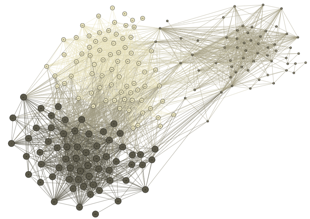 Figure 2
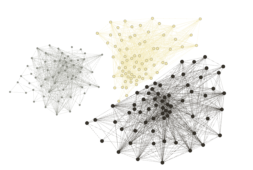 Figure 3
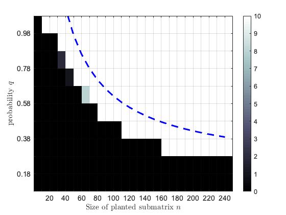 Figure 4
| Graph | Number of vertices | Number of edges | Size of dense subgraph | Running time |
|---|---|---|---|---|
| JAZZ | 198 | 2742 | 100 | 0.605735 sec |
| 1133 | 5451 | 289 | 20.139186 sec |
Peer Reviews
No public reviews on file for this paper yet. If you reviewed it on a platform where reviews are public (OpenReview, ICLR, NeurIPS, ICML), you can paste yours below so the community can read it here.
Code & Models
Videos
No videos yet. Explain this paper in a talk, walkthrough, or lecture? Add one.
Convex optimization for the densest subgraph and densest submatrix problems
Polina Bombina Department of Mathematics, University of Alabama, Tuscaloosa, Alabama, [email protected]
Brendan Ames University of Alabama, Tuscaloosa, Alabama, [email protected]
Abstract
We consider the densest -subgraph problem, which seeks to identify the -node subgraph of a given input graph with maximum number of edges. This problem is well-known to be NP-hard, by reduction to the maximum clique problem. We propose a new convex relaxation for the densest -subgraph problem, based on a nuclear norm relaxation of a low-rank plus sparse decomposition of the adjacency matrices of -node subgraphs to partially address this intractability. We establish that the densest -subgraph can be recovered with high probability from the optimal solution of this convex relaxation if the input graph is randomly sampled from a distribution of random graphs constructed to contain an especially dense -node subgraph with high probability. Specifically, the relaxation is exact when the edges of the input graph are added independently at random, with edges within a particular -node subgraph added with higher probability than other edges in the graph. We provide a sufficient condition on the size of this subgraph and the expected density under which the optimal solution of the proposed relaxation recovers this -node subgraph with high probability. Further, we propose a first-order method for solving this relaxation based on the alternating direction method of multipliers, and empirically confirm our predicted recovery thresholds using simulations involving randomly generated graphs, as well as graphs drawn from social and collaborative networks.
1 Introduction
We consider the densest -subgraph problem: given graph , identify the -node subgraph of of maximum density, i.e., maximum average degree. Equivalently, the problem reduces to finding the -node subgraph of with maximum number of edges. It is easy to see that the densest -subgraph problem is NP-hard by reduction to the maximum clique problem, well-known to be NP-hard [1]. Indeed, if contains a clique of size , it would induce the densest -subgraph of ; any polynomial time algorithm for densest -subgraph would immediately provide a polynomial-time algorithm for maximum clique. Moreover, it has been shown by [2, 3, 4] that the densest -subgraph problem does not admit polynomial-time approximation schemes in general. Despite this intractability, the identification of dense subgraphs plays a significant role in many practical applications, especially in the analysis of web graphs, and social and biological networks [5, 6, 7, 8, 9, 10].
We propose a new convex relaxation for the densest -subgraph problem to address this intractability. Although we do not, and should not, expect our algorithm to provide a good approximation of the densest -subgraph for all graphs, we will show that it is functionally equivalent to the densest -subgraph problem for a large class of program instances. In particular, suppose that the random input graph consists of a -node subgraph with edges added with significantly higher probability than those edges outside . We will show that if is sufficiently large then is the densest -subgraph of , and it can be recovered from the optimal solution of our convex relaxation.
This result can be thought of as a specialization of recent developments regarding the recovery of clusters in graphs. In graph clustering, one seeks to partition the nodes of a given graph into dense subgraphs. Several recent results [11, 12, 13, 14, 15, 16, 17, 18, 19, 20, 21, 22, 23, 24, 25, 26, 27, 28], among others, have established sufficient conditions on the generative model under which dense subgraphs can be recovered in a random graph, typically from the solution of some convex relaxation. These results assume that the random graph is generated using some generalization of the stochastic block model (see [29]), which assumes that the edges are added within blocks or clusters with higher frequency than between blocks, and provide sufficient conditions on the number and relative sizes of clusters, and the probabilities of adding edges that guarantee that the underlying block structure can be recovered in polynomial-time. The recent survey article [30] provides an overview of such recovery guarantees.
Relatively few analogous results exist for the densest -subgraph problem. Ames and Vavasis [31, 32] consider convex relaxations for the maximum clique problem. Given an input graph, the maximum clique problem aims to identify the largest clique in the graph, that is, the vertex set of the largest complete subgraph (see [33, 34] for further discussion of the maximum clique problem). Ames and Vavasis [31, 32] establish that the maximum clique can be recovered from the optimal solution of particular convex relaxation if the input graph consists of a single large complete graph that is obscured by noise in the form of random edge additions and deletions. In particular, both results show that hidden cliques of size at least can be identified with high probability for -node random graphs constructed so that the probability of adding an edge between nodes in the hidden clique is significantly higher than adding other potential edges to the graph. The notation indicates that there is some constant such that for all sufficiently large and we say that an event occurs with high probability if the probability of the event tends to polynomially as the size of the graph tends to . The latter result recasts the hidden clique problem as that of finding the densest -subgraph, where is the size of the hidden clique. Similar theoretical recovery guarantees can be found in [35, 36, 37, 38, 39, 40]. We delay the derivation of our convex relaxation and statement of the general recovery guarantee until Section 2.
We generalize these results for the densest subgraph problem to obtain an analogous recovery guarantee for the densest submatrix problem, which seeks to find the densest submatrix of given size. That is, we seek the submatrix of desired size with maximum number of nonzero entries. Similar results for the submatrix localization problem, where one seeks to find a block of entries with elevated mean in a random matrix, were presented in [41, 42, 43]. We will see that our convex relaxation correctly identifies the densest submatrix (of fixed size) in random matrices provided that entries within this submatrix are significantly more likely to be nonzero than an arbitrary entry of the matrix. We present our generalization of the densest subgraph problem to the densest submatrix problem and the statement of our theoretical recovery guarantees in Section 3. We provide proofs of our main results in Section 4 and conclude with discussion of a first-order method for solving our convex relaxations and empirical results illustrating efficacy of our approach in Section 5.
2 Relaxation of the Densest -Subgraph Problem and Perfect Recovery of a Planted Clique
Our relaxation hinges on the observation, made in [32], that the adjacency matrix of any subgraph of can represented as the difference of a rank-one matrix and a binary correction matrix; this observation is closely related to the sparse plus low-rank decomposition of clustered graphs first considered in [25, 44], although with the restriction to submatrices of the adjacency matrix. Let be a subset of nodes of . We denote by the subgraph induced by ; that is, is the graph with node set and edge set given by the subset of with both endpoints in . Let be the characteristic vector of : if and otherwise for all . The matrix is a rank-one binary matrix with nonzero entries indexed by . If is a complete subgraph, i.e., for all , then is equal to the sum of the adjacency matrix of and the binary diagonal matrix with nonzero entries indexed by ; we call this sum the perturbed adjacency matrix of , and denote it by .
If is not a complete subgraph, then there is some , such that . Let denote the set of all such . For each , we have , while . It follows that where is the projection onto the set of matrices having support contained in , defined by
[TABLE]
We call the matrix representation of the subgraph . The density of is given by
[TABLE]
where denotes the number of nonzero entries of , because is equal to twice the number of nonadjacent nodes in . Moreover, the entries of the correction matrix are binary, which implies that . Therefore, we may pose the densest -subgraph problem as the rank-constrained binary program
[TABLE]
where denotes the matrix trace function, and denotes the all-ones vector in . Unfortunately, combinatorial optimization problems involving rank and binary constraints are intractable in general. In particular, the densest -subgraph problem is NP-hard and, hence, we cannot expect to be able to solve (1) efficiently. Relaxing the rank constraint with a nuclear norm penalty term given by as in [45], the binary constraints with box constraints, and ignoring the symmetry constraints yields the convex program
[TABLE]
where is a regularization parameter chosen to control emphasis between the two objectives.
As mentioned earlier, we do not expect the solution of (2) to give a good approximation of the densest -subgraph for an arbitrary graph. We instead restrict our focus to those graphs which we can expect to to contain a single especially dense -subgraph with high probability.
Definition 2.1
We construct the edge set of a -node random graph as follows. Let be a -subset of nodes; for each , we add to independently with probability . For each , we add to independently with probability . We say such a graph is sampled from the planted dense -subgraph model.
This model, considered in [32], is a generalization of the planted clique model considered in [31], where is chosen to be . On the other hand, the planted dense -subgraph model is a special case of the generalized stochastic block model [44], corresponding to a graph with exactly one cluster of size and outlier nodes. Note that any graph sampled from the planted dense -subgraph contains a -subgraph, , with higher density than the rest of the graph in expectation. Our goal is to derive conditions on the size of this subgraph and the edge densities and that ensure recovery of the planted subgraph from the optimal solution of (2). The following theorem provides such a sufficient condition.
Theorem 2.1
Suppose that the -node graph is sampled from the planted dense -subgraph model with edge probabilities and respectively. Let denote the matrix representation of the planted dense -subgraph . Then constants exist such that if
[TABLE]
then is the unique optimal solution of (2) for penalty parameter
[TABLE]
and is the unique densest -subgraph of with high probability; here and are equal to the edge creation variances and inside and outside of the planted dense -subgraph, respectively.
Here, and in the rest of the paper, an event holding with high probability (w.h.p.), means that the event occurs with probability tending polynomially to one as ; that is, there are scalars such that the event occurs with probability at least . Note that (3) is only satisfiable when . To illustrate the contribution of Theorem 2.1 we consider a few choices of , and .
First, suppose that and are fixed so that the edge densities in are fixed as we vary . In this case, Theorem 2.1 states that we may recover , with high probability, provided that . This bound is identical to that found many times in the planted clique literature [31, 46, 47, 48, 35], up to constants and the logarithmic term. It is widely believed that finding planted cliques of size is intractable; indeed, several heuristic approaches have recently been proven to fail to recover planted cliques of size in polynomial-time [3, 2, 4] and this intractability has been exploited in cryptographic applications [49].
On the other hand, our bound shows that planted cliques of size much smaller than can be recovered in the presence of sparse noise. This should not be seen as a proof that we can recover planted cliques of size in general, but rather evidence of the intimate relationship between the size of hidden cliques recoverable and the noise obscuring them. If very little noise in the form of diversionary edges is hiding the signal, here the planted clique, we should expect the signal to be significantly easier to recover. This is reflected in the fact that we can recover significantly smaller cliques than in this setting. For example, let be a fixed constant and let vary with such that . The probability of adding an edge outside of tends to zero as . Further, the left-hand side of (3) tends to as , and the dominant term in the right-hand side is . This implies that we can have exact recovery of the hidden clique w.h.p. provided . This lower bound on the size of recoverable -subgraph matches that for identifying clusters in sparse graphs provided in the graph clustering literature, albeit for the case where the graph contains the single cluster indexed by surrounding by many outlier nodes (see [30] and the references within). Moreover, this lower bound improves significantly upon that given by [32], where it is shown to that is sufficient for exact recovery w.h.p. in the presence of sparse noise.
3 The Densest Submatrix Problem
The densest -subgraph problem is a specialization of the far more general densest submatrix problem. Let for each positive integer . Given a matrix , the densest -submatrix problem seeks subsets and of cardinality and , respectively, such that the submatrix with rows index by and columns indexed by contains the maximum number of nonzero entries. It should be clear that this specializes immediately to the densest -subgraph problem when the input matrix is the perturbed adjacency matrix of the input graph and . However, the densest -submatrix problem allows far more flexible problem settings.
For example, the densest submatrix problem also specializes immediately to the maximum edge/density biclique problem. Let be a bipartite graph. Given integer , the decision version of the maximum edge biclique problem determines if contains an biclique, i.e., whether there are vertex sets , of cardinality and such that each vertex in is adjacent to every vertex in . This problem immediately specializes to the densest -subgraph problem with equal to the -block of the adjacency matrix of . Similar specializations exist for finding the densest subgraph in directed graphs, hypergraphs, and so on.
Let denote the index set of zero entries of given matrix . Without loss of generality, we may assume that the entries of are binary. If not, then we may replace with the binary matrix having the same sparsity pattern without changing the index set of the densest -submatrix. We would like to obtain a rank-one matrix with nonzero entries with minimum number of disagreements on :
[TABLE]
where is used to count the number of disagreements between and . Relaxing binary and rank constraints as before, we obtain the convex relaxation
[TABLE]
where is a regularization parameter chosen to tune between the two objectives. As before, we should expect to recover the solution of (5) from that of (6) when contains a single large dense block. The following definition proposes a class of random matrices with this property.
Definition 3.1
We construct an random binary matrix as follows. Let and be and -index sets. For each and , we let with probability and [math] otherwise. For each remaining we set with probability and take otherwise. We say such a matrix is sampled from the planted dense -submatrix model.
The following theorem provides a sufficient condition for exact recovery of a planted dense -submatrix generalizing the analogous result for recovery of a planted dense -subgraph given by Theorem 2.1.
Theorem 3.1
Suppose that the matrix is sampled from the planted dense -subgraph model with edge probabilities and , respectively, with rows and columns of the planted dense subgraph indexed by and , respectively. Let denote the matrix representation of . Let and . Then there are constants such that if
[TABLE]
then is the unique optimal solution of (6) for penalty parameter for all , and is the unique densest -submatrix of with high probability.
In the case when and , the inequality (7) specializes to (3), although the constants should differ due to the lack of an assumption of symmetry of and in Theorem 3.1.
4 Derivation of the Recovery Guarantees
This section will consist of a proof of Theorem 3.1. The proof of Theorem 2.1 is identical except for minor modifications due to the symmetry of . We begin with the following theorem, which provides the required optimality conditions for (6).
Theorem 4.1
Let be a -subset of and let be a -subset of , and be their characteristic vectors. Then the solutions and are optimal for (6) if and only if there are dual multipliers , , , and satisfying
[TABLE]
The proof of Theorem 4.1 is nearly identical to that of [32, Theorem 4.1] and is omitted. Suppose that is sampled from the planted dense -subgraph model with edge probabilities . Our goal is to establish the conditions on given by Theorem 3.1 that guarantee exact recovery (w.h.p.) of the matrix representation of the planted submatrix with rows and columns given by and respectively. Our approach follows that of [32, Section 4]. We first explicitly construct dual multipliers and using the dual feasibility condition (8a) and the complementary slackness conditions (8b) and (8c). We then use the characterization of the subdifferential of the nuclear norm (8d) to construct the remaining dual variables . We conclude the proof by using concentration inequalities to establish feasibility of the proposed dual variables under the hypothesis of Theorem 2.1.
We choose and according to the dual feasibility condition (8a) so that the orthogonality conditions and are satisfied. We consider the following cases.
- Case 1. If , then (8a) implies that
[TABLE]
if we take and define
- Case 2. If , , and , then we have , so by (8c). It follows that in this case.
- Case 3. If such that then we take and .
- Case 4. If , such that , we take and .
- Case 5. If and such that , we take
[TABLE]
where denotes the number of nonzero entries in the th column of indexed by rows in . so that . By our choice of , we have
[TABLE]
- Case 6. If , , and then we take
[TABLE]
where denotes the number nonzero entries in the th row of indexed by columns in .
By our choice of and , we have for all and for all . We choose the remaining dual variables and so that for all and for all .
The orthogonality conditions and define a linear system with equations for the unknown entries of when all other dual variables are fixed. To obtain a particular solution of this underdetermined linear system, we make the additional assumption that has rank at most 2, taking the form for some and . Under this assumption, the conditions , and , yield the linear system
[TABLE]
where the vectors and are defined by for all and for all . It is easy to see that this system is singular with null space spanned by . However, it is also easy to see that the unique solution of
[TABLE]
is a solution of (9); see [32, Section 4.2] for further details. Applying the Sherman-Morrison-Woodbury Formula (see [50, Equation (2.1.4)]), we have
[TABLE]
The entries of and are binomial random variables corresponding to and independent Bernoulli trials ith probability of success , respectively. Therefore, we have
[TABLE]
Choosing for some to be chosen later ensures that the entries of are strictly positive in expectation.
We next describe how to choose so that the entries of and are positive with high probability. To do so, we will make repeated use of the following specialization of the classical Bernstein inequality to bound the sum of independent Bernoulli random variables (see, for example,[51, Section 2.8]).
Lemma 4.1
Let be a sequence of independent Bernoulli random variables, each with probability of success . Let be the binomially distributed random variable denoting the number of successes. Then
[TABLE]
Applying (13) with to each component of and and the union bound shows that
[TABLE]
for all and w.h.p., where . On the other hand, is equal to the number of nonzero entries in the block of . Therefore, is a binomially distributed random variable, with . Applying (13) with again establishes that
[TABLE]
w.h.p. It follows immediately that
[TABLE]
for each if (14) and (16) are satisfied. Following an identical argument, we see that
[TABLE]
if (15) and (16) hold. Substituting (17) and (18) into the formula for shows that
[TABLE]
for all , w.h.p.; here, we use the assumption that . Choosing
[TABLE]
ensures that the entries of are nonnegative w.h.p.
4.1 Nonnegativity of
We next establish conditions on the regularization parameter ensuring that the entries of the dual variable are nonnegative. Recall that takes value [math] or for all except those corresponding to Cases 4 through 6 in the choice of and .
We begin with Case 5 in the construction of and . Recall that
[TABLE]
if and such that . Since is a binomial random variable corresponding to independent Bernoulli trials with probability of success , applying Bernstein’s inequality (13) shows that , and, hence,
[TABLE]
w.h.p., where . Under the gap assumption
[TABLE]
and the choice of given by we see that
[TABLE]
w.h.p. for some constant . An identical bound holds for entries of corresponding to Case 6 by symmetry. Finally, the bound for Case 4 follows by substituting in (20) which establishes that if in this case. Applying the union bound over all entries in establishes that is nonnegative w.h.p. if and satisfy the gap assumption (21) and
[TABLE]
4.2 A bound on the matrix
To complete the proof, we derive a sufficient condition involving , and that ensures that , as constructed above, satisfies with high probability. To simplify our notation, we again make the assumption that and . Our analysis will translate superficially to the cases when and , and , and and . We bound using the triangle inequality and the decomposition , where if , and otherwise. To bound the norms of and , we will make repeated use of the following bound on the norm of a random matrix. Specifically, Lemma 4.2 is a special case of the matrix concentration inequality given by [52, Corollary 3.11] on the spectral norm of matrices with i.i.d. mean zero bounded entries.
Lemma 4.2
Let be a random matrix with i.i.d. mean zero entries having variance and satisfying . Let . Then there is a constant such that
[TABLE]
for all .
The following lemma provides the desired bound on .
Lemma 4.3
Suppose that the matrix is constructed according to Cases 1 through 6 for a matrix sampled from the planted dense submatrix model with and . Then there is a constant such that
[TABLE]
with high probability.
We delay the proof of Lemma 4.3 until Appendix A. The following lemma provides the required bound on . Our analysis follows a similar argument to that of [31, Section 4.2]; we include it here for completeness.
Lemma 4.4
Suppose that the matrix is constructed according to Cases 1 through 6 for a matrix sampled from the planted dense submatrix model with and . Let and . Assume that is bounded away from so that . Then exists constant such that
[TABLE]
with high probability.
It follows immediately from Lemmas 4.3 and 4.4 that
[TABLE]
w.h.p. On the other hand,
[TABLE]
where we obtain the first inequality by substituting the choice of given by (22) and the upper bound . We obtain the last inequality using the fact that . Further, we have
[TABLE]
Substituting back into (24), we see that
[TABLE]
w.h.p. Enforcing so that (21) holds and the right-hand side of (25) is bounded above by establishes Theorem 3.1. This completes the proof.
5 A First-Order Method Based on the Alternating Direction Method of Multipliers
We conclude with discussion of an optimization algorithm for solution of (6) based on the alternating direction method of multipliers (ADMM); see [53] for details regarding the ADMM. We first present a derivation of the method and then empirically validate its performance using randomly generated matrices and real-world collaboration and communication networks.
5.1 The Optimization Algorithm
To apply the ADMM to (2), we first introduce artificial variables , , to obtain the equivalent convex optimization problem
[TABLE]
where denote the constraint sets
[TABLE]
Here, is the indicator function of the set , such that if , and otherwise. We solve (26) iteratively using the ADMM. Specifically, we update each primal variable by minimizing the augmented Lagrangian in Gauss-Seidel fashion with respect to each primal variable. Then the dual variables are updated using the updated primal variables. The augmented Lagrangian of (26) is given by
[TABLE]
where is a regularization parameter chosen so that is strongly convex in each primal variable. Minimization of the augmented Lagrangian with respect to each of the artificial primal variables and is equvalent to projection onto each of the sets and ; each of these projections has an analytic expression.
We update using projection onto the nonnegative cone: is the matrix with th entry if and [math] otherwise. On the other hand, we update using the proximal function for the nuclear norm , which can be computed by applying the soft thresholding operator defined by to the vector of singular values. Here, is the vector whose entries are the signs of the corresponding entries of , denotes the vector whose entries are the magnitudes of the corresponding entries of , and the maximum denotes the vector of pairwise maximums. We declare the algorithm to have converged when the primal and dual residuals , and are smaller than a desired error tolerance. The steps of the algorithm are summarized in Algorithm 1111A MATLAB implementation of Algorithm 1 is available from http://bpames.people.ua.edu/software..
5.2 Random matrices
We empirically verified the theoretical phase transitions provided by Theorem 3.1 using matrices randomly sampled from the planted dense subgraph model with fixed noise edge probability and varied the submatrix size and in-submatrix probability . We perform two sets of experiments: one where the matrix is sparse outside the planted submatrix and another when the noise obscuring the planted submatrix is relatively dense. For the dense graph simulations, we choose and . In the sparse experiments, we choose and for ten equally spaced spanning the interval . For each set of simulations, we vary and set . In the sparse experiments, we have and we use in dense experiments. In both the dense and sparse graph simulations, we generate matrices according to the planted dense submatrix model for each choice of the parameters and (with remaining parameters , , and chosen as described above). We call Algorithm 1 to solve the instance of (6) corresponding to each randomly sampled matrix. The regularization parameter , augmented Lagrangian parameter , and stopping tolerance are used in each call of Algorithm 1. We declared the planted submatrix to be recovered if the relative error is less than , where is the solution returned by Algorithm 1 and is the matrix representation of the planted submatrix. The empirical probability of recovery of planted submatrix is plotted in Figure 1. Color of a square indicates rate of recovery in the corresponding simulations, with black corresponding to [math] and white corresponding to recoveries out of trials. The dashed curves show the phase transition to perfect recovery predicted by Theorem 3.1. The empirical recovery rates observed in these trials closely matches that predicted by Theorem 3.1. The discrepancy between the observed phased transition and that more conservatively predicted by Theorem 3.1 is due to the presence of the logarithmic terms in (3); a slight modification of our proof to follow that of [31, Theorem 7] eliminates these terms when and are constants and the gap is sufficiently large.
5.2.1 Collaboration and Communication Networks
We also applied our algorithm to identify communities in networks taken from the 10th DIMACs Implementation Challenge, which focused on graph partitioning and clustering [54, 55]. The first graph (JAZZ) represents a collaboration network with musicians and edges, and was compiled by [56]. Here, two musicians are connected if they have performed together. Earlier studies [10] showed that this network contains a cluster of musicians. We apply Algorithm 1 to the adjacency matrix of this network with regularization parameter , stopping tolerance , and . Our algorithm converges to the dense submatrix representing this community after iterations. Figure 2 is a visualization of this network using the software package Gephi [57] and the ForceAtlas2 algorithm [58]. The statistics function of Gephi is used to identify three communities within this network, including the community of size identified by Algorithm 1.
We also consider the graph (EMAIL) representing the network of e-mail interchanges between faculty, researchers, technicians, managers, administrators, and graduate students of the Univeristy Rovira i Virgili (Tarragona). Two individuals are connected if they exchanged an email. There are nodes and edges. From [59], we know that the EMAIL graph has a dense subgraph of vertices, representing a community of ; additionally, we can identify clusters using the statistics function of Gephi corresponding to academic units within this university, including this community. Applying Algorithm 1 with , , and stopping criteria finds this subgraph in iterations. The results of these analyses are summarized in Table 1.
6 Conclusions
We have presented an analysis of new convex relaxations for the densest subgraph and submatrix problems and have established sufficient conditions under which the optimal solution of original combinatorial problem coincides with that of these relaxations. In particular, these sufficient conditions characterize a signal-to-noise (SNR) ratio for matrices sampled from a particular distribution of random matrices, such that if this ratio is sufficiently large then we can expect to recover the combinatorial solution from the solution of the relaxation. Here, we expect perfect recovery if the strength of signal, as measured by the gap between probabilities of existence of nonzero within-group edges and out-group entries, is sufficiently larger than noise, as measured by variability of presence of nonzero entries. Further, the SNR corresponding to this phase transition to perfect recovery matches the current state of the art identified in the previous literature (up to constant and logarithmic terms); see [43].
This recovery guarantee provides a sufficient condition for perfect recovery of the planted subgraph or submatrix. It would be very interesting to determine if this condition is also necessary. For example, we establish that we have perfect recovery of planted dense -submatrices and subgraphs if when the probabilities , are sufficiently large constants. It is unclear if it is possible, either using our relaxation or some other method, to efficiently recover planted submatrices and subgraphs of size for some .
A secondary open problem focuses on efficient solution of the proposed convex relaxations. We currently solve these problems using a multi-block variant of the ADMM. Each iteration of this algorithm requires arithmetic operations; the bulk of these operations are used by the calculation of the singular value decomposition used to update . This per-iteration cost scales unfavorably when is large. The recent manuscript by Sotirov [60] proposed a coordinate descent heuristic for the densest -subgraph, with empirical evidence that this heuristic efficiently solves large-scale instances of the densest -subgraph problem. However, sufficient conditions for perfect recovery of a planted dense submatrix have not yet been established for this method has not been. Further research is needed to design efficient and scalable algorithms, i.e., with per-iteration cost , with provable theoretical guarantees of recovery for the solution of the densest subgraph and submatrix problems.
Acknowledgements. B. Ames was supported by University of Alabama Research Grants RG14678 and RG14838.
Appendix A Proof of Lemma 4.3
The proof is virtually identical to that of [32, Lemma 4.5]. We decompose as , where is matrix defined by if and otherwise. We can further decompose as where are constructed as below.
We first bound . Note that has i.i.d. mean-zero entries, with variance and values either with probability or with probability . Applying (23) with and ,
[TABLE]
w.h.p. Next, we let . Note that
[TABLE]
Applying (14) shows that for all w.h.p. It follows that
[TABLE]
w.h.p. Next, let . An identical argument shows that
[TABLE]
w.h.p. Finally, we let
[TABLE]
It is easy to confirm that . Applying (16) shows that
[TABLE]
w.h.p. Combining (27), (28), (29), and (30) establishes that
[TABLE]
w.h.p., as required.
Appendix B Proof of Lemma 4.4
To obtain the desired bound on , we first approximate with a random matrix with mean zero entries. In particular, we let be the random matrix constructed as follows. For all such that , or such that , we let . All remaining entries of are sampled independently from the generalized Bernoulli distribution , where sampled from satisfy
[TABLE]
Note that is a random matrix with i.i.d. mean zero entries sampled independently from by our choice of . Applying Lemma 4.2 shows that
[TABLE]
w.h.p. The remainder of the proof establishes that is well-approximated by , i.e., we complete the proof by bounding the norm of the error . We begin with the error in the block. Let . Applying Lemma 4.2 with again shows that
[TABLE]
w.h.p. We define by
[TABLE]
To bound the norm of , we will use the following lemma, which provides a bound on the spectral norm of random matrices of this form.
Lemma B.1
Let be an matrix whose entries are chosen according to with . Let be the random matrix defined by
[TABLE]
where is the number of ’s in the th column of . Then there are constants such that
[TABLE]
The proof of Lemma B.1 follows a similar argument to that of [31, Theorem 4] and is included as Appendix C. It is easy to see that the nonzero block has form as in the hypothesis of Lemma B.1. It follows that
[TABLE]
w.h.p. Similarly, we define the final correction matrix by
[TABLE]
Applying Lemma B.1 to the transpose of we have
[TABLE]
w.h.p. Combining (31), (32), (33), and (34) and applying the union bound completes the proof.
Appendix C Proof of Lemma B.1
The result relies on an application of the Matrix Bernstein Inequality; see [61, Theorem 6.1.1] and [62, Theorem 1.6] for further details. We first state the necessary bound on the spectral norm of the sum of finitely many independent, bounded random matrices.
Theorem C.1** (Matrix Bernstein Inequality)**
Let be a finite sequence of independent random matrices such that and for all almost surely. Let and let denote the matrix variance defined by
[TABLE]
Then
[TABLE]
for all .
The remainder of the proof consists of a specialization of this inequality to the special case . Indeed, let
[TABLE]
where denotes the th column of and denotes the th standard basis vector. It is clear that . It remains to estimate an upper bound on the spectral norms of the matrices and an upper bound on the variance . Once we have estimated these quantities, we will substitute them into (36) to complete the proof.
We begin with the following estimate on , which is an immediate consequence of the standard Bernstein Inequality (13).
Lemma C.1
There is a constant such that matrices defined by (37) satisfy
[TABLE]
for all with probability at least .
**Proof: ** Fix . Note that the . Moreover, the Bernstein Inequality (13) implies that
[TABLE]
with probability at least , where the last inequality follows from the fact that w.h.p. (by (13)) and (by the gap assumption). Taking the square root completes the proof.
We next bound the matrix variance .
Lemma C.2
The matrix defined by (37) satisfies for any constant satisfying for all .
**Proof: ** It suffices to construct upper bounds on each of and . We begin with the latter. Note that . This implies that is a diagonal matrix with th diagonal entry equal to . It follows that For each , we have
[TABLE]
where the inequality follows from the assumption that and the second to last inequality follows from the fact that is equal to the variance of the binomial variable . This implies that
[TABLE]
On the other hand, . It follows immediately that
[TABLE]
by the triangle inequality and Jensen’s inequality. Applying (38), we see that
[TABLE]
Substituting (39) and (41) into the formula for , we see that we have .
We are now ready to complete the proof of Lemma B.1. Let’s consider the following cases. First, suppose that and let in (36). Recall that applying the Bernstein Inequality (13) to each binomial variable implies that there is a constant such that for all with probability at least . This implies that we have with the same probability. Substituting into (36), along with the choice of from Lemma C.1, we see that
[TABLE]
using the assumption that . Rearranging further, we see that
[TABLE]
if we choose large enough that (which is possible if we impose the assumption that ).
Next, consider the case that and let . Then the Matrix Bernstein Inequality (36) implies that
[TABLE]
for any satisfying . Combining the two cases, we see that there are constants such that
[TABLE]
with probability at least . This completes the proof.
The reference list from the paper itself. Each links out to its DOI / PubMed record.
- 1[1] Karp, R.: Reducibility among combinatorial problems. Complexity of Computer Computations 40 (4), 85–103 (1972)
- 2[2] Alon, N., Arora, S., Manokaran, R., Moshkovitz, D., Weinstein, O.: Inapproximability of densest κ 𝜅 \kappa -subgraph from average case hardness. Unpublished manuscript 1 (2011)
- 3[3] Feige, U.: Relations between average case complexity and approximation complexity. In: Proceedings of the thiry-fourth annual ACM symposium on Theory of computing, pp. 534–543. ACM (2002)
- 4[4] Khot, S.: Ruling out ptas for graph min-bisection, dense k-subgraph, and bipartite clique. SIAM Journal on Computing 36 (4), 1025–1071 (2006)
- 5[5] Henzinger, M.R., Motwani, R., Silverstein, C.: Challenges in web search engines. In: ACM SIGIR Forum, vol. 36, pp. 11–22. ACM (2002)
- 6[6] Gibson, D., Kumar, R., Tomkins, A.: Discovering large dense subgraphs in massive graphs. In: Proceedings of the 31st international conference on Very large data bases, pp. 721–732. VLDB Endowment (2005)
- 7[7] Angel, A., Sarkas, N., Koudas, N., Srivastava, D.: Dense subgraph maintenance under streaming edge weight updates for real-time story identification. Proceedings of the VLDB Endowment 5 (6), 574–585 (2012)
- 8[8] Gajewar, A., Das Sarma, A.: Multi-skill collaborative teams based on densest subgraphs. In: Proceedings of the 2012 SIAM International Conference on Data Mining, pp. 165–176. SIAM (2012)
