Network design for s-t effective resistance
Pak Hay Chan, Lap Chi Lau, Aaron Schild, Sam Chiu-wai Wong, Hong Zhou

TL;DR
This paper studies the problem of designing a subgraph with limited edges to minimize the effective resistance between two nodes, providing hardness results and approximation algorithms, including a PTAS for series-parallel graphs.
Contribution
It introduces the first approximation algorithms and hardness results for the s-t effective resistance network design problem, bridging shortest path and flow problems.
Findings
The problem is NP-hard and hard to approximate within a factor of two.
A convex relaxation yields a constant factor approximation algorithm.
A PTAS exists for series-parallel graphs, improving approximation ratios.
Abstract
We consider a new problem of designing a network with small - effective resistance. In this problem, we are given an undirected graph , two designated vertices , and a budget . The goal is to choose a subgraph of with at most edges to minimize the - effective resistance. This problem is an interpolation between the shortest path problem and the minimum cost flow problem and has applications in electrical network design. We present several algorithmic and hardness results for this problem and its variants. On the hardness side, we show that the problem is NP-hard, and the weighted version is hard to approximate within a factor smaller than two assuming the small-set expansion conjecture. On the algorithmic side, we analyze a convex programming relaxation of the problem and design a constant factor approximation algorithm. The key of the…
Click any figure to enlarge with its caption.
 Figure 1
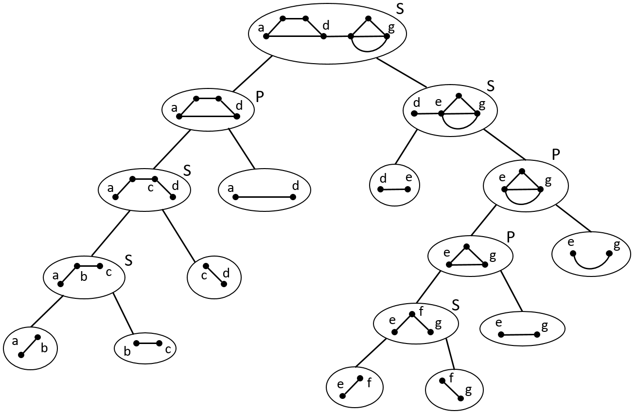 Figure 2
 Figure 3
 Figure 4
Peer Reviews
No public reviews on file for this paper yet. If you reviewed it on a platform where reviews are public (OpenReview, ICLR, NeurIPS, ICML), you can paste yours below so the community can read it here.
Videos
No videos yet. Explain this paper in a talk, walkthrough, or lecture? Add one.
Taxonomy
TopicsReliability and Maintenance Optimization · Sustainable Supply Chain Management · Complexity and Algorithms in Graphs
Network Design for - Effective Resistance
Pak Hay Chan111University of Waterloo. Email: [email protected], Lap Chi Lau222University of Waterloo. Supported by NSERC Discovery Grant 2950-120715 and NSERC Accelerator Supplement 2950-120719. Email: [email protected], Aaron Schild333University of California, Berkeley. Email: [email protected], Sam Chiu-wai Wong444Microsoft Research Redmond. Email: [email protected], Hong Zhou555University of Waterloo. Email: [email protected]
We consider a new problem of designing a network with small - effective resistance. In this problem, we are given an undirected graph , two designated vertices , and a budget . The goal is to choose a subgraph of with at most edges to minimize the - effective resistance. This problem is an interpolation between the shortest path problem and the minimum cost flow problem and has applications in electrical network design.
We present several algorithmic and hardness results for this problem and its variants. On the hardness side, we show that the problem is NP-hard, and the weighted version is hard to approximate within a factor smaller than two assuming the small-set expansion conjecture. On the algorithmic side, we analyze a convex programming relaxation of the problem and design a constant factor approximation algorithm. The key of the rounding algorithm is a randomized path-rounding procedure based on the optimality conditions and a flow decomposition of the fractional solution. We also use dynamic programming to obtain a fully polynomial time approximation scheme when the input graph is a series-parallel graph, with better approximation ratio than the integrality gap of the convex program for these graphs.
1 Introduction
Network design problems are generally about finding a minimum cost subgraph that satisfies certain “connectivity” requirements. The most well studied problem is the survivable network design problem [22, 1, 23, 25, 19], where the requirement is to have a specified number of edge-disjoint paths between every pair of vertices . Other combinatorial requirements are also well studied in the literature, including vertex connectivity [29, 15, 5, 10, 30, 7] and shortest path distances [12, 11].
Some spectral requirements are also studied, including spectral expansion [28, 2], total effective resistances [21, 35], and mixing time [4], but in general much less is known about these problems. See Section 1.1 for more discussions of previous work.
In this paper, we study a basic problem in designing networks with a spectral requirement – the effective resistance between two vertices.
Definition 1.1** (The - effective resistance network design problem).**
The input is an undirected graph , two specified vertices , and a budget . The goal is to find a subgraph of with at most edges that minimizes , where denotes the effective resistance between and in the subgraph . See Section 2.2 for the definition of effective resistance and Section 3.1 for a mathematical formulation of the problem.
The - effective resistance is an interpolation between - shortest path distance and - edge connectivity. To see this, let be a unit - flow in and define the -energy of as , and let - be the minimum -energy of a unit - flow that the graph can support. Thomson’s principle (see Section 2.2) states that , so that a graph of small - effective resistance can support a unit - flow with small -energy. Note that the shortest path distance between and is (as the -energy of a flow is just the average path length and is minimized by a shortest - path), and so a graph with small has a short path between and . Note also that the edge-connectivity between and is equal to the reciprocal of (because if there are edge-disjoint - paths, we can set the flow value on each path to be ), and so a graph with small has many edge-disjoint - paths. As is between and , the objective function takes both the - shortest path distance and the - edge-connectivity into consideration.
A simple property suggests that -energy may be even more desirable than and as a connectivity measure. Conceptually, adding an edge to would make and more connected. For and , however, adding would not yield a better energy if does not improve the shortest path and the edge connectivity respectively. In contrast, the -energy would typically improve after adding an edge, and so -energy provides a smoother quantitative measure that better captures our intuition how well and are connected in a network.
Traditionally, the effective resistance has many useful probabilistic interpretations, such as the commute time [6], the cover time [34], and the probability of an edge in a random spanning tree [27]. These interpretations suggest that the effective resistance is a useful distance function and have applications in the study of social networks. Recently, effective resistance has found surprising applications in solving problems about graph connectivity, including constructing spectral sparsifiers [40] (by using the effective resistance of an edge as the sampling probability), computing maximum flow [9], finding thin trees for ATSP [3], and generating random spanning trees [33, 39].
Thomson’s principle also states that the electrical flow between and is the unique flow that minimizes the -energy. So, designing a network with small - effective resistance has natural applications in designing electrical networks [13, 21, 24]. One natural formulation is to keep at most wires in the input electrical network to minimize , so that the electrical flow between and can still be sent with small energy while we switch off many wires in the electrical network.
Based on the above reasons, we believe that the effective resistance is a nice and natural alternative connectivity measure in network design. More generally, it is an interesting direction to develop techniques to solve network design problems with spectral requirements.
1.1 Main Results
Unlike the classical problems of shortest path and min-cost flow (corresponding to the and versions of the problem), the - effective resistance network design problem is NP-hard.
Theorem 1.2**.**
The - effective resistance network design problem is NP-hard.
On the other hand, we analyze a natural convex programming relaxation for the problem (Section 3.1), and use it to design a constant factor approximation algorithm for the problem.
Theorem 1.3**.**
There is a convex programming based -approximation randomized algorithm for the - effective resistance network design problem.
The algorithm crucially uses a nice characterization of the optimal solutions to the convex program (Lemma 3.2) to design a randomized path-rounding procedure (Section 3.2) for Theorem 1.3.
A simple example shows that the integrality gap of the convex program is at least two. When the budget is much larger than the length of a shortest - path, we show how to achieve an approximation ratio close to two with a randomized “short” path rounding algorithm (Section 3.5).
Theorem 1.4**.**
There is a -approximation algorithm for the - effective resistance network design problem, when where is the length of a shortest - path.
1.2 Other Results
We consider some variants of the - effective resistance network design problem, including the weighted version, the dual version, and the problem on special graphs.
There is a natural weighted generalization of the - effective resistance network design problem, where we associate a cost and resistance to each edge of the input graph.
Definition 1.5** (The weighted - effective resistance network design problem).**
The input is an undirected graph where each edge has a non-negative cost and a non-negative resistance , two specified vertices , and a cost budget . The goal is to find a subgraph of that minimizes subject to the constraint that the total edge cost of is at most . In the following, we may refer to this problem as the weighted problem for simplicity.
In the weighted problem, the integrality gap of the convex program (Section 3.1) becomes unbounded, even when the cost on the edges are the same ( for all ). This suggests that the weighted version may be strictly harder. Indeed, we show stronger hardness result for the weighted problem assuming the small-set expansion conjecture [37, 38].
Theorem 1.6**.**
Assuming the small-set expansion conjecture, it is NP-hard to approximate the weighted - effective resistance network design problem within a factor of for any , even when for every edge .
On the other hand, when the cost on the edges are the same, the following approximation follows from the randomized path rounding algorithm in a black box manner.
Corollary 1.7**.**
There is a convex programming based -approximation randomized algorithm for the weighted - effective resistance network design problem when for every edge , where is the ratio between the maximum and minimum resistance.
As our problem is related to electrical network design, it is natural to consider the special case when the input graph is a series-parallel graph. In this setting, we can use dynamic programming to design an exact algorithm for the original problem, and a fully polynomial time approximation scheme (FPTAS) for the weighted problem.
Theorem 1.8**.**
There is an exact algorithm for the - effective resistance network design problem with running time when the input graph is a series-parallel graph.
There is a -approximation algorithm for the weighted - effective resistance network design problem when the input graph is a series-parallel graph. The running time of the algorithm is where is the ratio between the maximum and minimum resistance. By a simple preprocessing scaling step, we can assume that is bounded by a polynomial, and so the algorithm is a FPTAS for the weighted problem.
We note that the integrality gap examples in Section 3.1 are actually series-parallel graphs, and so the dynamic programming algorithms go beyond the limitation of the natural convex program. We leave it as an open problem whether the weighted problem admits a constant factor approximation algorithm (possibly by combining these techniques).
We also consider the “dual” problem where we set the effective resistance as a hard constraint, and the objective is to minimize the number of edges in the solution subgraph. We present similar results as the original problem in Section 3.6.
1.3 Related Work
In the survivable network design problem, we are given an undirected graph and a connectivity requirement for every pair of vertices , and the goal is to find a minimum cost subgraph such that there are at least edge-disjoint paths for all . This problem is extensively studied and captures many interesting special cases [22, 1, 23, 19]. The best approximation algorithm for this problem is due to Jain [25], who introduced the technique of iterative rounding to design a -approximation algorithm. His result has been extended in various directions, including element-connectivity [16, 8], directed graphs [18, 19], and with degree constraints [31, 14, 17, 32].
Other combinatorial connectivity requirements were also considered. A natural variation is to require internally vertex disjoint paths for every pair of vertices . This problem is much harder to approximate [29, 30], but there are good approximation algorithms for global connectivity [15, 7] and when the maximum connectivity requirement is small [5, 10]. Another natural problem is to require a path of length between every pair of vertices . This problem is also hard to approximate in general but there are better approximation algorithms when every edge has the same cost and the same length [12].
Spectral connectivity requirements were also studied, including spectral gap [20, 28] (closely related to graph expansion), total effective resistances [21], and mixing time [4]. Some of the earlier works only proposed convex programming relaxations and heuristic algorithms. Approximation guarantees are only obtained in two recent papers for the more general experimental design problem. When every edge has the same cost, there is a -approximation algorithm for minimizing the total effective resistance when the budget is at least [35], and there is a -approximation algorithm for maximizing the spectral gap when the budget is at least [2]. For our problem, the interesting regime is when is much smaller than , where the techniques in [2, 35] do not apply. We have developed a set of new techniques for analyzing and rounding the solutions to the convex program that will hopefully find applications for solving related problems.
1.4 Techniques
Our main technical contribution is in designing rounding techniques for a convex programming relaxation of our problem. There is a natural convex programming relaxation, by using the conductance of the edges as variables, and writing the - effective resistance as the objective function and noting that it is convex with respect to the variables (Section 3.1).
We show that optimal solutions of this convex program enjoy some nice properties666We can also show that there exists an optimal solution such that the fractional edges form a forest, but this is not included in the paper as we have not used this property in the rounding algorithm.. Given an optimal fractional solution and the unit - electrical flow supported in , we derive from the KKT optimality conditions that there is a flow-conductance ratio such that for every fractional edge with and for every integral edge with . The flow-conductance ratio is crucial in the rounding algorithm and the analysis.
The rounding techniques in the two recent papers on experimental design [2, 35] considered each edge/vector as a unit. In [2], a potential function as in spectral sparsification is used to guide a local search algorithm to swap two edges/vectors at a time to improve the current solution. In [35], a probability distribution on the edges/vectors is carefully designed for an independent randomized rounding. These techniques are only known to work in the case when the solutions form a spanning set so that the “contribution” of each individual edge/vector is well-defined. This is basically the reason why the results in [2, 35] only apply when the budget is at least .
Our approach is based on a randomized rounding procedure on - paths. Given , we compute the unit - electrical flow supported in , and decompose as a convex combination of - paths. The rounding algorithm has iterations (recall that is the flow-conductance ratio of the optimal solution ), where we pick a random path from the convex combination in each iteration, and return as our solution. One difference from the previous techniques in the literature is that each unit in the rounding algorithm is a - path, so in particular and are always connected in our solution. Another difference is that our problem has some extra structure, so that we can compute the electrical flow to guide our rounding procedure, where the variables are not in the convex program. These allow us to obtain a constant factor approximation algorithm for all budget (note that when there is no feasible integral solution).
In the analysis, we prove in Lemma 3.6 that the expected number of edges in is at most , and in Lemma 3.7 that the expected effective resistance is . To bound the expected effective resistance, we use Thomson’s principle and construct a unit - flow to show that . To construct the unit - flow , we keep the flow-conductance ratio and send units of flow on each sampled path (i.e. and ). The flow-conductance ratio plays a crucial role in the proofs of both lemmas. This is because the rounding algorithm is based on the flow variables , and thus the performance guarantees are in terms of , but the ratio allows us to relate them back to the variables in the convex program. Combining the two lemmas give us a constant factor bicriteria approximation algorithm for the problem. This can be turned into a true approximation algorithm by scaling down the budget to and run the bicriteria approximation algorithm with some additional claims (Section 3.4).
The improvement on the approximation ratio when budget is large comes from two observations. The first is that if is much larger than the length of the shortest - path, then the number of independent iterations in the rounding scheme is large (Lemma 3.3). The second is that we can ignore some - paths in the flow decomposition with many fractional edges without affecting the performance much. Combining these, we can apply a Chernoff-Hoeffding bound to show that the number of edges is at most with high probability. Then it is not necessary to scale down the budget by a factor of and we can prove a stronger bound that the effective resistance is at most times the optimal value.
1.5 Organization
In Section 2, we define the notations used in this paper and cover background knowledge on effective resistances. We present the convex programming relaxation and our two rounding procedures in Section 3, and the dynamic programming algorithm in Section 4. The NP-hardness and small set expansion hardness results are provided in Section 5.
2 Preliminaries
We introduce the notations and definitions for graphs and matrices in Section 2.1, and then define electrical flow and effective resistance and state some basic results in Section 2.2.
2.1 Graphs and Matrices
Let be an undirected graph with edge weight on each edge . The number of vertices and the number of edges are denoted by and . For a subset of edges , the total weight of edges in is . For a subset of vertices , the set of edges with one endpoint in and one endpoint in is denoted by . For a vertex , the set of edges incident on a vertex is , and the weighted degree of is . The volume of a set is defined as the sum of the weighted degrees of vertices in . The conductance of a set is defined as the ratio of the total weight on the boundary of to the total weighted degrees in . For two subsets , the set of edges with one endpoint in and one endpoint in is denoted by .
In this paper, an undirected graph with non-negative edge weights is interpreted as an electrical network, where each edge is a resistor with conductance (not to be confused with the conductance of a set as defined above), or equivalently with resistance . The adjacency matrix of the graph is defined as for all . The Laplacian matrix of the graph is defined as where is the diagonal degree matrix with for all . For each edge , let where is the vector with one in the -th entry and zero otherwise. The Laplacian matrix can also be written as
[TABLE]
Let be the eigenvalues of with corresponding orthonormal eigenvectors so that . It is well-known that the Laplacian matrix is positive semidefinite and with as the corresponding eigenvector, and if and only if is connected. The pseudo-inverse of the Laplacian matrix of a connected graph is defined as
[TABLE]
which maps every vector orthogonal to to a vector such that .
2.2 Electrical Flow and Effective Resistance
Before defining - electrical flow, we first define the standard unit - flow. For each edge , we have two variables and with , where is positive if the flow is going from to and negative otherwise. A unit - flow satisfies the following flow conservation constraints:
[TABLE]
Given a unit - flow , we overload the notation and define its undirected flow vector with for each edge . A unit - electrical flow is a unit - flow that also satisfies the Ohm’s law: There exists a potential vector such that for all ,
[TABLE]
The effective resistance between and is defined as
[TABLE]
which is the potential difference between and when one unit of electrical flow is sent from to . The - effective resistance can be interpreted as the resistance of the whole graph as a big resistor when an electrical flow is sent from to .
One can write the effective resistance in terms of the Laplacian matrix. For , let b_{uv}=\mathrm{\raisebox{1.9919pt}{\chi}}_{u}-\mathrm{\raisebox{1.9919pt}{\chi}}_{v}, where \mathrm{\raisebox{1.9919pt}{\chi}}_{v}\in\mathbb{R}^{n} is the unit vector with in the -th entry and [math] in other entries. Combining the flow conservation constraint and the Ohm’s law, it can be checked that the potential vector of a unit - electrical flow is a solution to the linear system
[TABLE]
Note that is a solution, and if is connected then any solution is given by for . Therefore, we can write
[TABLE]
The effective resistance can also be characterized by the energy of a flow. The energy of an - flow is defined as
[TABLE]
Thomson’s principle [26] states that the unit - electrical flow is the unique unit - flow that minimizes the energy. This can be verified by writing down the optimality condition of the minimization problem. Moreover, this energy is exactly the - effective resistance. To see this, note that the flow value on edge in the unit - electrical flow satisfies and thus
[TABLE]
To summarize, we will use the following result from Thomson’s principle.
Fact 2.1** (Thomson’s principle [26]).**
Let be the unit electrical - flow in . Then
[TABLE]
A corollary of Thomson’s principle is the following intuitive result known as the Rayleigh’s monotonicity principle.
Fact 2.2** (Rayleigh’s monotonicity principle).**
The - effective resistance cannot increase if the resistance of an edge is decreased.
We will also use the following result to write a convex programming relaxation of our problem.
Fact 2.3** ([21]).**
The - effective resistance is a convex function with respect to the conductance of the edges.
3 Convex Programming Algorithm
In this section, we analyze a convex programming relaxation for our problem. We first describe the convex program and prove a characterization of the optimal solutions in Section 3.1. We then present a randomized rounding algorithm using flow decomposition in Section 3.2, and show that it is a constant factor bicriteria approximation algorithm in Section 3.3. Then, we show how to convert the bicriteria approximation algorithm into a true approximation algorithm in Section 3.4, and how to modify the algorithm slightly to achieve a better approximation guarantee when the budget is large in Section 3.5. Finally, we discuss the dual problem of minimizing the cost while satisfying the effective resistance constraint in Section 3.6.
3.1 Convex Programming Relaxation
The formulation is for the weighted problem, where each edge has a weight . We introduce a variable for each edge to indicate whether is chosen in our subgraph. Let
[TABLE]
be the Laplacian matrix of the fractional solution , and be the - effective resistance of the graph with conductance on edge . The following is a natural convex programming relaxation for the problem.
[TABLE]
This is an exact formulation if for all . The objective function is convex in by Fact 2.3. The convex program can be solved in polynomial time by the ellipsoid method to inverse exponential accuracy, or by the techniques described in [2] to inverse polynomial accuracy, which are both sufficient for the rounding algorithm.
3.1.1 Integrality Gap Examples
We show some limitations of the convex program for general and . The following figure shows a simple example where the integrality gap is unbounded if the cost could be arbitrary.
In this graph, the top path has length where each edge has cost . The bottom path has two edges with cost . The resistance of each edge is , and the budget is . The integrality gap of this example is . To see this, the integral solution can only afford the top path, and the effective resistance is . However, the fractional solution can set for each of the two bottom edges, and the effective resistance of this fractional solution is .
The following figure shows another simple example where the integrality gap is unbounded if the edge costs are the same but the resistances could be arbitrary.
In this example, the top path has length with each edge of resistance . The bottom path has only one edge with resistance . All edges have cost and the budget . The integral solution can only afford the bottom path, with effective resistance . The fractional solution can set for each edge in the top path, with effective resistance . When , the integrality gap could be arbitrarily large.
Even in the unit-cost unit-resistance case, the integrality gap is unbounded if is smaller than the - shortest path distance. Henceforth, in view of these observations we assume the following in the rest of this section.
Assumption 3.1**.**
We assume that for every edge , which is the setting of the - effective resistance network design problem, and the budget is at least the shortest path distance between and in the input graph.
The integrality gap of the convex program is still at least two with Assumption 3.1. For a simple example, consider a graph with two vertex-disjoint - paths, each of length , and the budget is . Then the optimal integral value is while the optimal fractional value is close to , and so the integrality gap gets arbitrarily close to two.
We will show that the integrality gap of the convex program is at most with these assumptions. Note that just to connect and , then must be at least the - shortest path distance. It is interesting that this small additional assumption could reduce the integrality gap from unbounded to a constant.
3.1.2 Characterization of Optimal Solutions
In the case for all edges , we will prove that the electrical flow supported in the optimal solution to (CP) satisfies a crucial property about the flow-conductance ratio .
Lemma 3.2** (Characterization of Optimal Solution).**
Let be the input graph with for all edges . Let be an optimal solution to the convex program (CP). Let be the set of fractional edges with , and be the set of integral edges with . Let be the undirected flow vector of the unit - electrical flow supported in . There exists such that
[TABLE]
Proof.
By removing edges with , we can assume for every . By removing isolated vertices, we can further assume that the nonzero edges form a connected graph. So, we can write , where has rank and the null space of is . Since , we have and , which implies that where is the all-ones matrix. Using the fact that (see e.g. [36]), we derive
[TABLE]
where we used the assumption that for all . With this, we write down the KKT conditions for the convex program. Let be the dual variable for the budget constraint , and and be the dual variables for the upper bound and the nonnegative constraint respectively. The KKT conditions states if is an optimal solution to (CP), then there exist and such that
[TABLE]
where we used the assumption that for all . For an integral edge with , we have by the complementary slackness condition. Since , it follows from the Lagrangian optimality condition that . For a fractional edge with , we have by the complementary slackness condition, and therefore by the Lagrangian optimality condition. We can assume that . Otherwise, implies that the flow on all fractional edges are zero, and so we can delete them from the graph without affecting the - effective resistance, and we have an integral solution.
Let be a potential vector of the electrical flow supported in . For an edge ,
[TABLE]
where the first equality is by Ohm’s law and the assumption that for all , and the second equality uses that as explained in Section 2.2. The lemma then follows from the above paragraph and writing as . ∎
The flow-conductance ratio will be crucial in the rounding algorithm and its analysis. The following lemma shows an upper bound on using the budget and the shortest path distance between and .
Lemma 3.3**.**
Under the conditions in Assumption 3.1, it holds that .
Proof.
Let be an optimal solution to (CP), and be the unit - electrical flow supported in . As , a shortest path is a feasible solution to (CP), and thus . On the other hand, by Thomson’s principle and Lemma 3.2,
[TABLE]
where the last equality holds since we can assume for the optimal solution without loss of generality by Rayleigh’s principle (or otherwise we have an integral optimal solution). The lemma follows by combining the upper bound and the lower bound. ∎
3.2 Randomized Path-Rounding Algorithm
Our rounding algorithm uses the unit electrical flow supported in the optimal solution to construct an integral solution. The algorithm will first decompose the flow as a convex combination of flow paths, and then randomly choose the flow paths and return the union of the chosen flow paths as our solution.
The following lemma about flow decomposition is by the standard argument to remove one (fractional) flow path at a time, which holds for any unit directed acyclic - flow.
Lemma 3.4** (Flow Decomposition).**
Given a unit - electrical flow , there is a polynomial time algorithm to find a set of - paths with such that the undirected flow vector can be written as a convex combination of the characteristic vectors of the paths in , i.e.
[TABLE]
where is the characteristic vector of the path with one on each edge and zero otherwise.
With the flow decomposition, we are ready to present the rounding algorithm.
Randomized Path Rounding Algorithm
Let be an optimal solution to the convex program (CP). Let be the unit - electrical flow supported in . Let be the flow-conductance ratio defined in Lemma 3.2. 2. 2.
Compute a flow decomposition of as defined in Lemma 3.4. 3. 3.
For from to do
- •
Let be a random path from where each path is sampled with probability . 4. 4.
Return the subgraph formed by the edge set .
The following lemma shows that the rounding algorithm will always return a non-empty subgraph.
Lemma 3.5**.**
Suppose the input instance satisfies the conditions in Assumption 3.1. Let be an optimal solution to (CP) and be the flow-conductance ratio as defined in Lemma 3.2. Then
[TABLE]
Proof.
Since we assumed that the budget is at least the length of a shortest - path, it follows from Lemma 3.3 that . This implies that
[TABLE]
∎
3.3 Bicriteria Approximation
The analysis of the approximation guarantee goes as follows. First, we show that the expected number of edge in the returned subgraph is at most the budget . Then, we prove that the expected effective resistance of the returned subgraph is at most two times that of the optimal fractional solution. Both of these steps use the flow-conductance ratio crucially. These combine to show that the randomized path rounding algorithm is a constant factor bicriteria approximation algorithm.
Let be an optimal solution to (CP). Let and be the set of fractional edges and integral edges in . We assume that each edge will be included in the subgraph returned by the rounding algorithm. We focus on bounding the number of edges in that will be included in .
Lemma 3.6** (Expected Budget).**
Let be an optimal solution to (CP) when for all edges . Let be an indicator variable of whether is included in the returned subgraph by the rounding algorithm, Then,
[TABLE]
Proof.
Note that an edge is contained in with probability . By the union bound, an edge is included in the returned subgraph by the rounding algorithm with probability
[TABLE]
where the last equality holds by the property of the flow decomposition of the electrical flow in Lemma 3.4.
By Lemma 3.2, for each fractional edge , and this implies that
[TABLE]
Therefore,
[TABLE]
∎
The key step is to show that . To prove this, we construct a unit - flow and show that , and hence by Thomson’s principle . To construct the flow , the idea is to follow the ratio in the fractional solution and send units of flow on each path selected.
Lemma 3.7** (Expected Effective Resistance).**
Suppose the input instance satisfies the conditions in Assumption 3.1. Let be an optimal solution to (CP) and be the unit - electrical flow supported in . The expected - effective resistance of the subgraph returned by the rounding algorithm is
[TABLE]
Proof.
Consider the undirected flow vector defined by sending units of flow on each path chosen by the rounding algorithm, i.e. the random variable with for each edge . We would like to upper bound the expected energy in order to upper bound .
Each is a random - path sampled from the flow decomposition of the undirected flow vector of the unit - electrical flow supported in , and is its characteristic vector with expected value
[TABLE]
Since each edge in is of conductance one, the expected energy of in is
[TABLE]
As each path is sampled independently, for ,
[TABLE]
For ,
[TABLE]
where the last equality follows from the property of the flow decomposition in Lemma 3.4. Combining these two terms, it follows that
[TABLE]
Thomson’s principle states that the is upper bounded by the energy of any one unit - flow. Note that is an - flow of units, and by Lemma 3.5. Scaling to a one unit - flow by dividing the flow on each edge by gives an upper bound on
[TABLE]
where the second inequality follows from Lemma 3.2 that for every edge and also for every edge , and the last equality is from Thomson’s principle that . Finally, notice that as . ∎
Combining Lemma 3.6 and Lemma 3.7, it follows from a simple application of Markov’s inequality that there is an outcome of the randomized path-rounding algorithm which uses at most edges with - effective resistance at most . In the following, we apply Markov’s inequality more carefully to show that the success probability is at least . In the next subsection, we will argue that can be assumed to be and so the path-rounding algorithm is a randomized polynomial time algorithm.
Theorem 3.8** (Bicriteria Approximation).**
Suppose the input instance satisfies the conditions in Assumption 3.1. Let be an optimal solution to (CP). Given , the randomized path rounding algorithm will return a subgraph with at most edges and with probability at least .
Proof.
First, we bound the probability that the subgraph has more than edges. Let be an indicator variable of whether the edge is included in the returned subgraph . Recall that and denote the set of fractional edges and integral edges in respectively. We assume pessimistically that all edges in will be included in the subgraph returned by the rounding algorithm. Then, by Markov’s inequality and Lemma 3.6,
[TABLE]
where the last inequality is by .
Next, we bound the probability that . By Markov’s inequality and Lemma 3.7,
[TABLE]
where the last inequality is because .
To prove the lemma, it remains to show that
[TABLE]
which follows from Lemma 3.5. ∎
3.4 Constant Factor Approximation
We showed that the randomized path rounding algorithm is a bicriteria approximation algorithm. To achieve a true approximation algorithm, a natural idea is to scale down the budget from to and apply the randomized path rounding algorithm. The following lemma takes care of the case of , when the shortest path assumption does not hold after scaling, by showing that simply returning a shortest - path is already a good enough approximation.
Lemma 3.9**.**
When the budget is at least the length of a shortest - path, any - shortest path is a -approximate solution for the - effective resistance network design problem.
Proof.
When , a - shortest path is a feasible solution to the problem with - effective resistance at most . To prove the lemma, we will show that for any feasible solution to (CP), and so an - shortest path is already a -approximation.
Let be the graph with fractional conductance on each edge . To show a lower bound on , we identify the vertices in to a form a path graph as follows: For each , let be the set of vertices in with shortest path distance to , where the shortest path distance is defined where each edge in is of length one. First, for each , we identify the vertices in to a single vertex . Then, we identify all the vertices in to a single vertex . The path graph has vertex set and edge set . For each edge in , its conductance in is the same as that in . As an electrical network, identifying two vertices is equivalent to adding an edge of resistance zero between and . So, it follows from Rayleigh’s monotonicity principle (Fact 2.2) that as and .
As is a series-parallel graph, we can compute directly. For each , let be the set of parallel edges connecting and in , and be the effective conductance between and in . Then, by Fact 4.3,
[TABLE]
Note that for any feasible solution . Using Cauchy-Schwarz inequality,
[TABLE]
Therefore, we conclude that . ∎
We are ready to prove our main approximation result.
Theorem 3.10**.**
Suppose the input instance satisfies the conditions in Assumption 3.1. There is a polynomial time -approximation algorithm for the - effective resistance network design problem.
Proof.
If the budget , then Lemma 3.9 shows that simply returning an - shortest path would give a -approximation. Henceforth, we assume .
Let be the objective value of an optimal solution to the convex program (CP) with budget , so . As is a feasible solution to (CP) with budget , by Thomson’s principle,
[TABLE]
Given the original budget , our algorithm is to find an optimal solution to (CP) with budget , and use the path-rounding algorithm with input to return a subgraph . By Theorem 3.8, with probability , the subgraph satisfies
[TABLE]
and so is an -approximate solution to the - effective resistance network design problem.
Finally, we consider the time complexity of the algorithm. The number of iterations in the path rounding algorithm is , and we need to run the path rounding algorithm times to boost the success probability to a constant. This is a randomized polynomial time algorithm when .
In the following, we show that when , it is easy to obtain a -approximate solution without running the path-rounding algorithm. Let be an optimal solution to (CP) with budget , and be the unit - electrical flow supported in . Let be the flow decomposition of as in Lemma 3.4. We call a path an integral path if every edge has ; otherwise we call a fractional path. When , we simply return the union of all integral paths as our solution . Clearly, has at most edges as it only contains integral edges. Next, we bound by the energy of the flow supported in the integral paths. By Lemma 3.2, an edge with has . This implies that each fractional path has . Since has at most paths (Lemma 3.4), the total flow in the fractional paths is at most , and thus the total flow in the integral paths is at least . By scaling the flow supported in the integral paths to a one unit - flow, we see that
[TABLE]
To summarize, in all cases including and , there is a polynomial time algorithm to return an -approximate solution to the - effective resistance network design problem. ∎
We make two remarks about improvements of Theorem 3.10.
Remark 3.11** (Approximation Ratio).**
The analysis of the 8-approximation algorithm is not tight. By a more careful analysis of the expected energy in Lemma 3.7 and the short path idea used in the next subsection, we can show that the approximation guarantee of the same algorithm in Theorem 3.10 is less than . However, the analysis is quite involved and not very insightful, so we have decided to omit those details and only keep the current analysis.
Remark 3.12** (Deterministic Algorithm).**
Using the standard pessimistic estimator technique, we can derandomize the path-rounding algorithm to obtain a deterministic -approximation algorithm. The analysis is standard and we omit the details that would take a few pages.
3.5 The Large Budget Case
In this subsection, we show how to modify the algorithm in Theorem 3.10 to achieve a better approximation ratio when the budget is much larger than the - shortest path distance.
The observation is that when , then is small by Lemma 3.3, and so there are many iterations in the path-rounding algorithm. Since each iteration is independent, we can use Chernoff-Hoeffding’s bound to prove a stronger bound on the probability that the number of edges in the returned solution is significantly more than (which outperforms the bound proved in Lemma 3.6 using Markov’s inequality). We can then show that the expected - effective resistance is close to two times the optimal value by arguments similar to the proof of Lemma 3.7.
Modified Rounding Algorithm
For our analysis, we slightly modify the path-rounding algorithm to ignore “long” paths in the flow decomposition, so that we have a worst case bound to apply Chernoff-Hoeffding’s bound. Unlike the flow decomposition in Lemma 3.4, the short path flow decomposition definition is specific to the electrical flow of an optimal solution to (CP). In the following definition, is a parameter which will be set to be to achieve a -approximation.
Definition 3.13** (Short Path Decomposition of Electrical Flow of Optimal Solution).**
Let be an optimal solution to the convex program (CP). Let be the unit - electrical flow supported in . Let be the flow-conductance ratio defined in Lemma 3.2.
Let be a flow decomposition of as defined in Lemma 3.4. Let be the total fractional value on the fractional edges in the optimal solution .
We call a path a long path if has at least edges in , i.e. . Otherwise we call a path a short path.
Let be the collection of short paths in . Let be the - flow defined by the short paths, and be the total flow value of .
The modified algorithm is very similar to the randomized path-rounding algorithm in Section 3.3. The only difference is that we only sample the paths in the short path flow decomposition in Definition 3.13, and we adjust the sampling probability of a path to so that the sum is one.
Randomized Short Path Rounding Algorithm
Let be an optimal solution to the convex program (CP). Let be the unit - electrical flow supported in . Let be the flow-conductance ratio defined in Lemma 3.2. 2. 2.
Compute a short path flow decomposition of as described in Definition 3.13. 3. 3.
For from to do
- •
Let be a random path from where each path is sampled with probability . 4. 4.
Return the subgraph formed by the edge set .
The following simple lemma shows that the total flow on the long paths is negligible when is large, which will be useful in the analysis.
Lemma 3.14**.**
For the short path flow decomposition in Definition 3.13, .
Proof.
Using for from Lemma 3.2 and the properties of the flow decomposition of in Lemma 3.4,
[TABLE]
where the last inequality is by the definition of long paths and the last equality is because is a unit - flow. ∎
Analysis of Approximation Guarantee
First, we consider the expected - effective resistance of the returned subgraph . For intuition, we can think of the modified rounding algorithm as applying the rounding algorithm in the scaled flow , and so it should follow from Lemma 3.7 that
[TABLE]
which will be at most when from Lemma 3.14.
We cannot directly apply Lemma 3.7 as stated, as the flow does not satisfy the flow-conductance ratio in Lemma 3.2, but essentially the same proof will work to get the same conclusion (but not exactly the same intermediate step).
Lemma 3.15**.**
Suppose the input instance satisfies the conditions in Assumption 3.1. Let be an optimal solution to (CP) and be the unit - electrical flow supported in . The expected - effective resistance of the subgraph returned by the randomized short path rounding algorithm is
[TABLE]
where is the short path flow decomposition of as described in Definition 3.13.
The main difference of the analysis is to apply the following Hoeffding’s inequality (instead of Markov’s inequality) to bound the probability that the returned subgraph has significantly more than edges.
Fact 3.16** (Hoeffding’s Inequality).**
Let be independent random variables. Let , and , then for any ,
[TABLE]
Lemma 3.17**.**
Suppose the input instance satisfies the conditions in Assumption 3.1. Let be an optimal solution to (CP) and be the unit - electrical flow supported in . Let be the subgraph returned by the randomized short path rounding algorithm given as input, and be the number of edges in . Then, for any ,
[TABLE]
where is the parameter in the short path flow decomposition in Definition 3.13 and is the flow-conductance ratio of and as defined in Lemma 3.2.
Proof.
As in Lemma 3.6, we assume pessimistically that all integral edges will be included in , and so we focus on the fractional edges . Let be the indicator variable of whether the edge is sampled in the -th iteration of the short path rounding algorithm, and be the total number of fractional edges sampled in the -th iteration. Let be the total number of fractional edges in . Note that , since if some fractional edge was sampled in different iterations, we only count it once in . By linearity of expectation, .
Let be the flow path decomposition of in Lemma 3.4, and be the short path flow decomposition of as described in Definition 3.13. For an edge , recall that is the total flow value on from the short paths in . As we scaled the probability of each path by in the rounding algorithm, the probability that edge is sampled in the -th iteration is . Let be the total flow value on from the long paths in . The expected value of is
[TABLE]
By the definition of the long paths,
[TABLE]
where we recall that . Therefore,
[TABLE]
where the last inequality uses that and . It follows that .
As each iteration is independent, the random variables for are independent. Since we only use short paths, the maximum value of each is at most . So we can apply Hoeffding’s inequality to show that
[TABLE]
Let be the total number of integral edges in . As , we conclude that
[TABLE]
∎
As in Section 3.3, we can combine Lemma 3.17 and Lemma 3.15 to show that the randomized short path rounding algorithm is a bicriteria approximation algorithm.
Theorem 3.18**.**
Suppose the input instance satisfies the conditions in Assumption 3.1. Suppose further that , where is an error parameter satisfying for a small constant . Let be an optimal solution to (CP). Given , the randomized short path rounding algorithm with will return a subgraph with at most edges and with probability at least .
Proof.
The additional assumption implies that by Lemma 3.3.
Setting and , it follows from Lemma 3.17 that
[TABLE]
where the last inequality holds for .
Since , Lemma 3.14 implies that for the short path flow decomposition in Definition 3.13. Using Markov’s inequality and Lemma 3.15, for sufficiently small we have
[TABLE]
Therefore, with probability at least , the subgraph returned by the randomized short path rounding algorithm satisfies both properties. ∎
Using the same arguments as in Section 3.4, we can turn the above bicriteria approximation algorithm into a true approximation algorithm.
Theorem 3.19**.**
Suppose the input instance satisfies the conditions in Assumption 3.1. Suppose further that , where is an error parameter satisfying for a small constant . There is a polynomial time -approximation algorithm for the - effective resistance network design problem.
Proof.
As in the proof of Theorem 3.10, we apply the bicriteria approximation algorithm in Theorem 3.18 with input , an optimal solution to (CP) with the scaled-down budget , to return a subgraph . As the new budget is still greater than , by Theorem 3.18, with probability at least the subgraph satisfies and
[TABLE]
where we used the notations and arguments in Theorem 3.10.
For the time complexity, note that by Lemma 3.3 and the large budget assumption, and so we can assume that , as otherwise there is a simple -approximation algorithm in the case described in Theorem 3.10. Therefore, the success probability can be boosted to a constant in polynomial number of executions of the bicriteria algorithm in Theorem 3.18. ∎
3.6 Cost Minimization with - Effective Resistance Constraint
In this subsection, we consider a “dual” problem of the - effective resistance minimization problem. In the dual problem, we are given a graph and a target effective resistance , and the objective is to find a subgraph of minimum number of edges such that . The same NP-hardness proof in Section 5.1 can be used to show that the dual problem is NP-complete.
Using the same techniques for the - effective resistance minimization problem, we can obtain a constant factor bicriteria approximation algorithm for this problem. As the proofs are very similar, we will just state the results and highlight the differences. The main difference is that the convex program has unbounded integrality gap, and as a consequence we cannot turn the bicriteria approximation algorithm into a true approximation algorithm as in the - effective resistance network design problem. Using the same technique as in Theorem 3.10, however, we can return an -approximation to the optimal number of edges without violating the effective resistance constraint, if we are allowed to buy up to four copies of the same edge (see Theorem 3.20).
Convex Programming Relaxation
We consider the following natural convex programming relaxation for the dual problem.
[TABLE]
Integrality Gap Examples
Unlike the - effective resistance network design problem, the convex program (DCP) has unbounded integrality gap. Consider the following example in Figure 3.3, where the top path has length , and the bottom path has only one edge. The target effective resistance is for some constant . Since , to satisfy the effective resistance constraint, any integral solution must contain both paths and thus has cost . However, the fractional solution can set for each edge in the top path and set for the bottom edge. It can be checked that this fractional solution satisfies the constraint, and the total cost is 1+. Therefore, the integrality gap of this example is .
Optimal Solutions
Although the convex program (DCP) has a large integrality gap, the same rounding technique can be used to obtain a constant factor bicriteria approximation algorithm. Exactly the same characterization of the optimality conditions as in the - effective resistance network design problem holds, such that any optimal solution satisfies the flow-conductance ratio as described in Lemma 3.2.
Analogous to Lemma 3.3, we can prove an upper bound on that
[TABLE]
Analogous to Lemma 3.9, we can prove a lower bound on any optimal solution that
[TABLE]
We can assume that , as otherwise a shortest - path is an optimal solution, and so we can assume that .
Rounding Algorithm
The rounding algorithm is exactly the same as in Section 3.3. The same proofs as in Lemma 3.6 and Lemma 3.7 will imply that, with probability , the subgraph returned by the randomized path rounding algorithm satisfies
[TABLE]
where is an optimal solution to (DCP) and so . The same lower bound on as described in Theorem 3.10 applies, and so this is a randomized polynomial time algorithm.
An Alternative Bicriteria Approximation Algorithm
In the - effective resistance network design problem, we turn a bicriteria approximation algorithm into a true approximation algorithm, by scaling down the budget by a factor of two and running the bicriteria approximation algorithm. For the proof, we argue by scaling down an optimal solution with budget to a solution with budget .
In the dual problem, we can also try a similar approach, by scaling down the target effective resistance by a factor of and run the bicriteria approximation algorithm. However, we cannot argue that , as an optimal solution with effective resistance may not be able to scale up to with effective resistance because of the capacity constraints for . This approach would work if we are allowed to violate the capacity constraint by a factor of .
Theorem 3.20**.**
Given an weighted input graph , there is a polynomial time algorithm for the dual problem which returns a multi-subgraph with and where there are at most parallel copies of each edge.
4 Dynamic Programming Algorithms for Series-Parallel Graphs
In this section, we will present the dynamic programming algorithms for solving the weighted - effective resistance network design problem on series-parallel graphs. We first review the definitions of series-parallel graphs in Section 4.1. Then, we present the exact algorithm in Theorem 1.8 when every edge has the same cost in Section 4.2, and the fully polynomial time approximation scheme in Theorem 1.8 in Section 4.3.
4.1 Series-Parallel Graphs
Definition 4.1** (two-terminal series-parallel graph).**
A two-terminal series-parallel graph (SP graph) is a graph with two distinguished vertices (the source and the target ) that can be constructed recursively as follows:
- •
Base case: A single edge
- •
Compose step: If and are two series parallel graphs with source and target (), then we can combine them in two ways:
- –
Series-composition: We identify with as the same vertex, the source of the new graph is and the target is .
- –
Parallel-composition: We identify with as the same vertex and with as the same vertex, the new source is and the new target is .
Given the sequence of steps of constructing a series-parallel graph , we can define a tree (SP-tree) as follows.
Definition 4.2** (SP-tree).**
- •
Leaf node: If is a single edge, then is a single node containing the edge.
- •
Recurse step: is either a series-composition (S) or a parallel-composition (P) of and , then is a S-node (P-node) containing , and its children are roots of the SP-trees of and .
For a tree node in a SP-tree , let be the subgraph that represents, be the two terminals of , and be its left and right child if is an internal node. Note that the SP-tree is a fully binary tree with nodes.
Given a two-terminal SP graph, the corresponding SP-tree can be computed in time. The linear time SP-graph recognition algorithm in [41] will give us the construction sequence of , and we can build the SP-tree bottom-up.
4.2 Exact Algorithm for Unit-Cost
The following fact shows that the weighted - effective resistance can be computed easily from the SP-tree.
Fact 4.3** (Resistance of series-parallel network).**
Let be a two-terminal SP graph and each edge has a non-negative resistance . Let be the corresponding SP-tree. For every tree node , we can compute the source-target effective resistance as follows.
- Leaf node: if is a leaf node with a single edge .
- S-node: .
- P-node:
We design the dynamic programming algorithm by defining the subproblems using the SP-tree . For every tree node and , we define the subproblem
[TABLE]
Since we assume that every edge has cost , there are at most subproblems, as the SP-tree has at most nodes and there are at most possibilities for the cost of a subgraph.
It follows from the definition that would be the optimal - effective resistance for our problem. To compute , with Fact 4.3, we can use the following recurrence which exhausts all possible distributions of the budget among the two children:
[TABLE]
As there are subproblems and each subproblem can be computed in time, the time complexity of this dynamic programming algorithm is .
4.3 Fully Polynomial Time Approximation Scheme
In this subsection, we use dynamic programming to design a fully polynomial time approximation scheme to prove Theorem 1.8. In the previous subsection, we assume that every edge has the same cost to obtain an exact algorithm, by having a bounded number of subproblems in dynamic programming. When the cost could be arbitrary, the number of subproblems can no longer be bounded by a polynomial. Since the cost constraint must be satisfied, we do not change the cost of the edges, but instead discretize the resistance of the edges and optimize over the cost. We show that this gives an arbitrarily good approximation provided that the discretization is fine enough.
Rescaling: First, by rescaling we assume that and in . Let and where is the error in the approximation guarantee. We further rescale the resistance by setting . This rescaling ensures that for any subgraph of in which - is connected, the - effective resistance is upper bounded by (when all the edges are in series) and is lower bounded by (when all the edges are in parallel).
Subproblems and Recurrence: Let be the SP-tree of and let be the root of . We define two similar sets of subproblems. For every tree node and a value , we define the subproblem
[TABLE]
Similar to the reasoning in the previous subsection, the subproblems satisfy the following recurrence relation:
[TABLE]
Discretized subproblems: We cannot use dynamic programming to solve the above recurrence relation efficiently as there are unbounded number of subproblems. Instead, we use dynamic programming to compute the solution of all the “discretized” subproblems using the same recurrence relation. For every integer from to , we define
[TABLE]
We can think of as the minimum cost required to select a subset of edges such that the effective resistance between and is at most , when the effective resistance is rounded up to an integer during each step of the computation in the recurrence relation.
Algorithm and Complexity: After computing all , the algorithm will return
[TABLE]
as the approximate minimum - effective resistance. Given a tree node , by trying all possible integral values of and , we can compute the values of for each possible in time. Therefore, the total running time of computing all is . To output the optimal edge set, we can store the optimal values of for each pair of to reconstruct the edge set.
Correctness and Approximation Guarantee: Since we have not changed the edge cost, the solution returned by the algorithm will have total cost at most . It remains to show that the - effective resistance is at most times the optimal - effective resistance. For every tree node and every , we define
[TABLE]
It follows from the definitions that the optimal - effective resistance is , and the output of our algorithm will be . The following lemma establishes the approximation guarantee.
Lemma 4.4**.**
For every tree node and for every , it holds that
[TABLE]
Proof.
We prove the lemma by induction on the tree node of the SP-tree.
Base Case: Suppose is a leaf node of and is a graph of a single edge .
- •
For , we have .
- •
For , we have and
[TABLE]
where the second inequality uses the fact that every resistance is at least , and the last equality uses and .
S-node: Suppose is a S-node. For every , we have
[TABLE]
where the first inequality follows from the induction hypothesis, and the second inequality follows from the fact that .
P-node: Suppose is a P-node. For every , we have
[TABLE]
where the first inequality follows from the induction hypothesis and the fact that , and the last inequality holds as the minimum resistance of any subgraph is at least .
Therefore, the lemma follows by induction on the SP-tree. ∎
By substituting and , we have
[TABLE]
which completes the proof of Theorem 1.8.
5 Hardness Results
In this section, we first prove that the - effective resistance network design problem is NP-hard in Section 5.1. Then, we prove that the weighted problem is APX-hard assuming the small-set expansion conjecture in Section 5.2.
5.1 NP-Hardness
We will prove Theorem 1.2 in this subsection. The following is the decision version of the problem.
Problem 5.1** (- effective resistance network design).**
- Input:* An undirected graph , two vertices , and two parameters and .*
- Question:* Does there exist a subgraph of with at most edges and ?*
We will show that this problem is NP-complete by a reduction from the 3-Dimensional Matching (3DM) problem.
Problem 5.2** (3-Dimensional Matching).**
- Input:* Three disjoint sets of elements ; a set of triples where each triple contains exactly one element in .*
- Question:* Does there exist a subset of pairwise disjoint triples in ?*
Reduction: Given an instance of 3DM with , let and denote the triples by .
We construct a graph as follows:
- Vertex Set: The vertex set is the disjoint union of five sets , , and . Each vertex in corresponds to a triple in , that is . Each vertex in corresponds to an element in , that is . Let . The set consists of “dummy” vertices . So, there are totally vertices in , which is polynomial in the input size of the 3DM instance.
- Edge Set: The edge set is the disjoint union of three edge sets , and . There are edges in , where we have three edges , and for each triple . There are edges in , where there is an edge from each vertex in to . There are edges in , where there is a path for each triple , . So, there are totally edges in , which is polynomial in the input size of the 3DM instance.
The following claim completes the proof of Theorem 1.2.
Lemma 5.3**.**
Let and . The 3DM instance has disjoint triples if and only if the graph has a subgraph with at most edges and .
Proof.
One direction is easy. If there are disjoint triples in the 3DM instance, say , then will consist of the paths , the edges in incident on , and all the edges in . There are edges in , and , as in the graph in Figure 5.6.
The other direction is more interesting. If there do not exist disjoint triples in the 3DM instance, then we need to argue that for any with at most edges. First, note that , and so the budget is not enough for us to buy more than paths. As it is useless to buy only a proper subset of a path, we can thus assume that consists of paths and all the edges in . has a total of exactly edges. For any such , we will argue that . Without loss of generality, assume that consists of and all edges in and . As are not disjoint, there are some vertices in that are not neighbors of . Call those vertices .
We consider the following modifications of to obtain , and use to lower bound . For every pair of vertices in , we add an edge of zero resistance. For each edge incident on , we decrease its resistance to zero. By the monotonicity principle, the modifications will not increase the - effective resistance, as we either add edges with zero resistance or decrease the resistance of existing edges. The modifications are equivalent to contracting the vertices with zero resistance edges in between, and so is equivalent to the graph in Figure 5.6. Therefore, we have .
We will prove that one of the inequalities in must be strict when (Figure 5.7). To argue the strict inequality, we look at the unit - electrical flow in and consider two cases.
- •
If there exists some vertex with no incoming electrical flow, then we can delete such a vertex without changing . But then in the modified graph , the number of parallel edges to is now strictly smaller than , and therefore .
- •
If there exists some vertex with some incoming electrical flow, then for some . Since we have decreased the resistance of such an edge to 0, the energy of in is strictly smaller than the energy of in . By Thomson’s principle, we have .
Since the 3DM instance has no disjoint triples, it follows that and thus one of the above two cases must apply. In either case, we have and this completes the proof of the other direction. ∎
5.2 Improved Hardness Assuming Small-Set Expansion Conjecture
In this subsection, we will prove Theorem 1.6 that it is NP-hard to approximate the weighted - effective resistance network design problem within a factor smaller than . First, we will state the small-set expansion conjecture and its variant on bipartite graphs, and present an overview of the proof in Section 5.2.1. Next, we will reduce the bipartite small-set expansion problem to the weighted - effective resistance network design problem in Section 5.2.2, and then reduce the small-set expansion problem to the bipartite small-set expansion problem in Section 5.2.3 to complete the proof.
5.2.1 The Small-Set Expansion Conjecture and Proof Overview
The gap small-set expansion problem is formulated by Raghavendra and Steurer [37]. We use the version stated in [38].
Definition 5.4** (Gap Small-Set Expansion Problem [37, 38]).**
Given an undirected graph , two parameters and , the -gap -small-set expansion problem, denoted by , is to distinguish between the following two cases.
- •
Yes*: There exists a subset with and .*
- •
No*: Every subset with has .*
It is conjectured in [37] that the gap small-set expansion problem becomes harder when becomes smaller.
Conjecture 5.5** (Small-Set Expansion Conjecture [37, 38]).**
For any , there exists sufficiently small such that is NP-hard even for regular graphs.
It is known that the small-set expansion conjecture implies the Unique Game conjecture [37] and is equivalent to some variant of the Unique Game Conjecture [38].
We will show the SSE-hardness of the weighted - effective resistance network design problem in two steps, and use the small-set expansion problem on regular bipartite graphs as an intermediate problem.
Proposition 5.6**.**
For any , there is a polynomial time reduction from on -regular graphs to on -regular bipartite graphs.
Proposition 5.7**.**
Given an instance of on a -regular bipartite graph , there is a polynomial time algorithm to construct an instance of the weighted - effective resistance network design problem with graph and cost budget satisfying the following properties.
- •
If is a Yes-instance, then there is a subgraph of with cost at most and
[TABLE]
- •
if is a No-instance, then every subgraph of with cost at most has
[TABLE]
Theorem 1.6 will follow immediately from the two propositions.
Theorem 5.8**.**
For any , it is NP-hard to approximate the weighted - effective resistance network design problem to within a factor of , assuming that is NP-hard on regular graphs for sufficiently small .
Proof.
First, given a -regular instance of , we apply Proposition 5.6 to obtain a -regular bipartite instance of . Then, we apply Proposition 5.7 with and and see that the ratio between the - effective resistance of the No-case and the Yes-case is at least
[TABLE]
for sufficiently small . ∎
We will prove Proposition 5.7 in Section 5.2.2 and Proposition 5.6 in Section 5.2.3.
5.2.2 From Bipartite Small-Set Expansion to weighted - Effective Resistance Network Design
We prove Proposition 5.7 in this subsection. In the Yes-case of bipartite SSE, we use the small dense subgraph (from the small low conductance set) to construct a small subgraph with small - effective resistance. In the No-case of bipartite SSE, we argue that every small subgraph has considerably larger - effective resistance.
Construction: Given an instance with a -regular bipartite graph , we construct an instance of the weighted - effective resistance network design problem with graph as follows. See Figure 5.8 for an illustration.
- Vertex Set: The vertex set of is simply the disjoint union of .
- Edge Set: The edge set of is the disjoint union of three edge sets . The edge set has edges, where there is an edge from to each vertex . The edge set has edges, where there is an edge from each vertex to .
- Costs and Resistances: Every edge in has and . Every edge has and .
- Budget: The cost budget is .
Yes**-case:** Suppose is a Yes-instance of . Since is regular, there exist subsets and such that and . We construct the subgraph of as follows.
- Subgraph : The subgraph includes all the edges from to , all the edges from to , and all the edges from to . Since edges from to are of cost zero, the total cost in is equal to .
The following claim will complete the proof of the first item of Proposition 5.7.
Lemma 5.9**.**
.
Proof.
Since is a -regular bipartite graph, we have
[TABLE]
where denotes the set of edges with one endpoint in and one endpoint in . Since , we have . Hence, the number of edges between and is
[TABLE]
In terms of - effective resistance, is equivalent to the graph in Figure 5.9, where is the set of vertices not in and . Since the edges from to and from to have zero resistance and edges between and have resistance one, we have . ∎
No**-case:** We will prove the second item of Proposition 5.7 by arguing that every subgraph of with total cost at most has considerably larger - effective resistance. Since all the edges between and have zero cost and adding edges never increases - effective resistance (by Rayleigh’s monotonicity principle), we can assume without loss of generality that any solution to the weighted - effective resistance network design problem takes all edges between and and also takes exactly edges from . Consider an arbitrary subgraph with the above properties. Let be the set of neighbors of and be the set of neighbors of , with . Let . Note that as we are in the No-case where for every . Using the same calculation as above, we have
[TABLE]
The subgraph is shown in Figure 5.10, where is the set of vertices not in and , and the edges within are not shown. To lower bound , we modify to obtain and argue that and then show a lower bound on .
To obtain from , we simply identify the three subsets of vertices to three vertices, which is equivalent to adding a clique of zero resistance edges to each of these three subsets. By Rayleigh’s monotonicity principle, this could only decrease the - effective resistance and so we have .
In terms of - effective resistance, the subgraph is equivalent to the graph with two paths between and (with parallel edges): one path of length one with parallel edges between and , another path of length two with parallel edges between and and parallel edges between and . To lower bound , we lower bound the resistance of and , denoted by and . Note that
[TABLE]
For , let and , then
[TABLE]
where the inequality holds since for any , and the last equality holds because . Finally, by Fact 4.3,
[TABLE]
where the last inequality is because we are in the No-case. This completes the proof of the second item of Proposition 5.7.
Remark 5.10**.**
In this subsection, we show the hardness of the weighted - effective resistance network design problem, when the edge cost and the edge resistance could be arbitrary. Using a similar argument as in the proof of Theorem 1.2, the reduction can be modified to the unit-cost case if we replace the edges from to and to by sufficiently long paths (so that the cost of connecting to a vertex in is much larger than the cost of connecting a vertex in to a vertex in ). Therefore, the same -SSE-hardness also holds in the case when every edge has the same cost.
5.2.3 From Small Set Expansion to Bipartite Small Set Expansion
We prove Proposition 5.6 in this subsection.
Construction: Given an instance on a -regular graph , we construct a -regular bipartite graph as follows. For each vertex in , we create a vertex and a vertex , so that . For each edge , we add two edges and to . It is clear from the construction that is -regular.
Correctness: To prove Proposition 5.6, we will establish the following two claims.
Yes**-case:** If there is a set with and in , then there exist and with and in . 2. 2.
No**-case:** If every set with has in , then every sets and with has in .
Yes**-case:** Let be a subset with and in . Let and , with . By construction, an edge if and only if both and are in , and thus . Since and is -regular, we have
[TABLE]
No**-case:** Consider arbitrary subsets and with . To lower bound , we will upper bound . We partition into groups where every group except the last group is of size and the last group is of size at most . We partition into groups in a similar way. The following claim uses the small-set expansion property in to show that there is no small dense subset in .
Lemma 5.11**.**
Suppose is a No-instance of . Then, for any and ,
[TABLE]
Proof.
We first argue that there is no small dense subset in , and then we will use it to bound . Suppose with . As is a No-instance, we know that and thus . Since , it follows that . Note that this also implies trivially that for any with .
Given and , let . In words, is the set of vertices in which have at least one copy in in . Since each and is of size at most , it follows that . Also, note that , as each edge in corresponds to one edge in while each edge in is corresponded to at most two edges in . Therefore, we can apply the bound in the previous paragraph to conclude that . ∎
We now use the lemma to bound . Since , it follows that and , and therefore
[TABLE]
As is bipartite,
[TABLE]
Therefore, we have
[TABLE]
This completes the proof of Proposition 5.6. We remark that a more careful argument gives and thus , but this constant does not matter for the proof of Theorem 5.8.
6 Concluding Remarks
We have formulated a new and natural network design problem and presented some hardness and algorithmic results. It opens up a number of interesting problems to be studied.
For the - effective resistance network design problem, we conjecture that the integrality gap of the convex program is exactly two. As mentioned in Remark 3.11, the analysis of the -approximation is not tight, and we can show that the same algorithm achieves an approximation ratio strictly smaller than . It would be good to close the gap completely. 2. 2.
The weighted case of arbitrary costs and arbitrary resistances is wide open. It will be interesting if there are stronger convex programming relaxations for the problem (perhaps adding some knapsack constraint as suggested by the dynamic programming algorithms for series-parallel graphs). 3. 3.
As in survivable network design, one could study the general problem when there are multiple source-sink pairs and each pair has a different effective resistance requirement. It will be very interesting if it is still possible to achieve a constant factor approximation in this general setting. 4. 4.
An interesting intermediate problem is to find a minimum cost network so that the maximum effective resistance over pairs (the resistance diameter) is minimized. This is an analog of the global connectivity problem in traditional network design.
A more open-ended direction is to unify and extend the techniques for network design problems with spectral requirements.
The reference list from the paper itself. Each links out to its DOI / PubMed record.
- 1[1] Ajit Agrawal, Philip Klein, and R Ravi. When trees collide: An approximation algorithm for the generalized steiner problem on networks. SIAM Journal on Computing , 24(3):440–456, 1995.
- 2[2] Zeyuan Allen-Zhu, Yuanzhi Li, Aarti Singh, and Yining Wang. Near-optimal discrete optimization for experimental design: A regret minimization approach. ar Xiv preprint ar Xiv:1711.05174 , 2017.
- 3[3] Nima Anari and Shayan Oveis Gharan. Effective-resistance-reducing flows, spectrally thin trees, and asymmetric tsp. In Foundations of Computer Science (FOCS), 2015 IEEE 56th Annual Symposium on , pages 20–39. IEEE, 2015.
- 4[4] Stephen Boyd, Persi Diaconis, and Lin Xiao. Fastest mixing markov chain on a graph. SIAM review , 46(4):667–689, 2004.
- 5[5] Tanmoy Chakraborty, Julia Chuzhoy, and Sanjeev Khanna. Network design for vertex connectivity. In Proceedings of the fortieth annual ACM symposium on Theory of computing , pages 167–176. ACM, 2008.
- 6[6] Ashok K Chandra, Prabhakar Raghavan, Walter L Ruzzo, Roman Smolensky, and Prasoon Tiwari. The electrical resistance of a graph captures its commute and cover times. Computational Complexity , 6(4):312–340, 1996.
- 7[7] Joseph Cheriyan and László A Végh. Approximating minimum-cost k-node connected subgraphs via independence-free graphs. SIAM Journal on Computing , 43(4):1342–1362, 2014.
- 8[8] Joseph Cheriyan, Santosh Vempala, and Adrian Vetta. Network design via iterative rounding of setpair relaxations. Combinatorica , 26(3):255–275, 2006.