Contextuality Test of the Nonclassicality of Variational Quantum Eigensolvers
William M. Kirby, Peter J. Love

TL;DR
This paper introduces a practical test for assessing the nonclassicality of variational quantum eigolvers (VQEs) through contextuality, revealing that some experimental VQEs exhibit quantum features while others do not.
Contribution
We develop an efficiently computable contextuality test for VQEs and apply it to experimental data to evaluate their quantum nature.
Findings
Some VQE implementations are contextual, indicating quantum behavior.
Not all experimental VQEs pass the contextuality test, suggesting classical features.
The test provides a new way to verify quantum resources in VQEs.
Abstract
Contextuality is an indicator of non-classicality, and a resource for various quantum procedures. In this paper, we use contextuality to evaluate the variational quantum eigensolver (VQE), one of the most promising tools for near-term quantum simulation. We present an efficiently computable test to determine whether or not the objective function for a VQE procedure is contextual. We apply this test to evaluate the contextuality of experimental implementations of VQE, and determine that several, but not all, fail this test of quantumness.
Click any figure to enlarge with its caption.
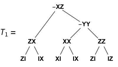 Figure 1
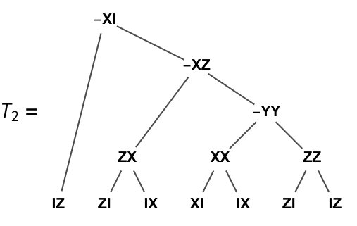 Figure 2
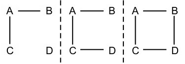 Figure 3
 Figure 4
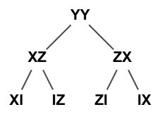 Figure 5
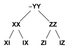 Figure 6
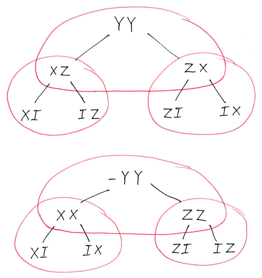 Figure 7
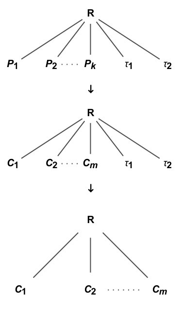 Figure 8
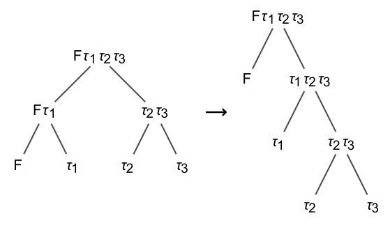 Figure 9
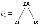 Figure 10
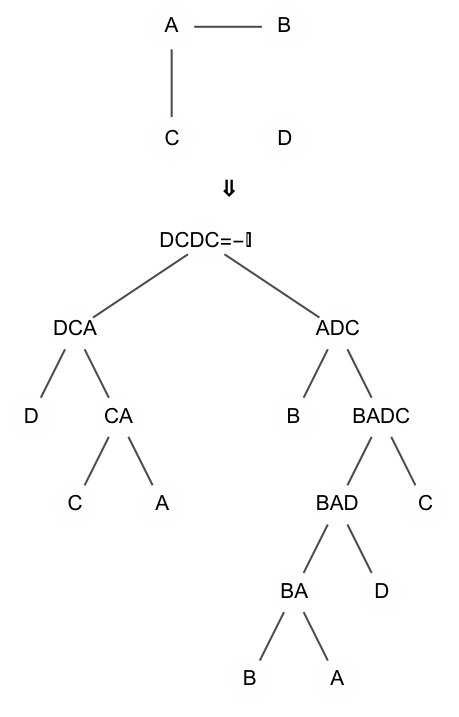 Figure 11
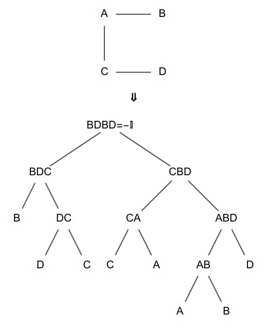 Figure 12
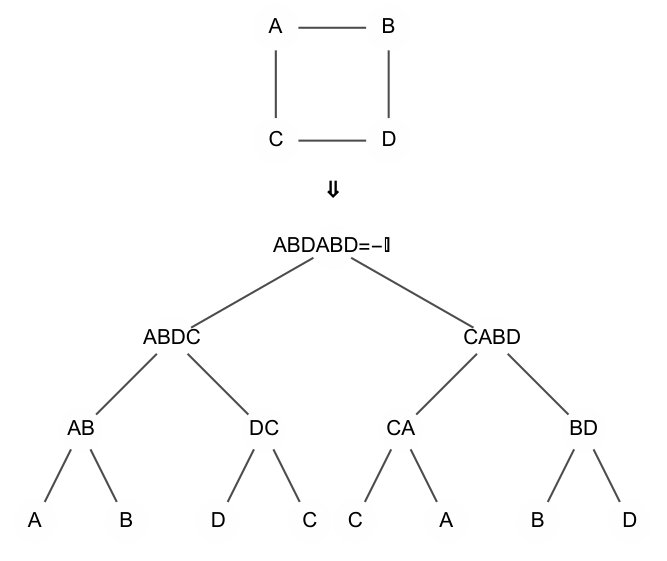 Figure 13
| Citation: | System: | Contextual? | ||
|---|---|---|---|---|
| Dumitrescu et al. Dumitrescu et al. (2018) | Deuteron | No | 0 | — |
| Kandala et al. Kandala et al. (2017) | H2 | No | 0 | 4 |
| O’Malley et al. O’Malley et al. (2016) | H2 | No | 0 | 5 |
| Hempel et al. Hempel et al. (2018) | H2 (BK) | No | 0 | 5 |
| Hempel et al. Hempel et al. (2018) | H2 (JW) | No | 0 | 14 |
| Colless et al. Colless et al. (2018) | H2 | No | 0 | 5 |
| Kokail et al. Kokail et al. (2019) | Schwinger Model | Yes | 0.14 | 231 |
| Nam et al. Nam et al. (2019) | O | Yes | 0.27 | 22 |
| Hempel et al. Hempel et al. (2018) | LiH | Yes | 0.33 | 13 |
| Peruzzo et al. Peruzzo et al. (2014) | HeH+ | Yes | 0.38 | 8 |
| Kandala et al. Kandala et al. (2017) | BeH | Yes | 0.74 | 164 |
| Kandala et al. Kandala et al. (2017, 2019) | LiH | Yes | 0.77 | 99 |
| Citation: | System | Contextual? | Encoding | ||
|---|---|---|---|---|---|
| Dumitrescu et al., 2018 Dumitrescu et al. (2018) | Deuteron | various333In Dumitrescu et al. (2018), Dumitrescu et al. compute the ground-state energies of the deuteron for effective field theories with dimension for (), and extrapolate from these to the infinite-dimensional space. Thus, is different for each value of . For , . For , . For , . All of these are noncontextual. | No | 0 | JW |
| Kandala et al., 2017 Kandala et al. (2017) | H2 | 4 | No | 0 | hybrid |
| O’Malley et al., 2016 O’Malley et al. (2016) | H2 | 5 | No | 0 | BK |
| Hempel et al., 2018 Hempel et al. (2018) | H2 | 5 | No | 0 | BK |
| Hempel et al., 2018 Hempel et al. (2018) | H2 | 14 | No | 0 | JW |
| Colless et al., 2018 Colless et al. (2018) | H2 | 5 | No | 0 | BK |
| Kokail et al., 2018 Kokail et al. (2019) | Lattice Schwinger Model | 231 | Yes | 0.16 | JW |
| Nam et al., 2019 Nam et al. (2019) | O | 22 | Yes | 0.27 | JW |
| Hempel et al., 2018 Hempel et al. (2018) | LiH | 13 | Yes | 0.33 | BK |
| Peruzzo et al., 2014 Peruzzo et al. (2014) | HeH+ | 8 | Yes | 0.38 | JW |
| Kandala et al., 2017 Kandala et al. (2017) | BeH | 164 | Yes | 0.74 | hybrid |
| Kandala et al., 2017/19 Kandala et al. (2017, 2019) | LiH | 99 | Yes | 0.77 | hybrid |
Peer Reviews
No public reviews on file for this paper yet. If you reviewed it on a platform where reviews are public (OpenReview, ICLR, NeurIPS, ICML), you can paste yours below so the community can read it here.
Videos
No videos yet. Explain this paper in a talk, walkthrough, or lecture? Add one.
Contextuality Test of the Nonclassicality of Variational Quantum Eigensolvers
William M. Kirby
Department of Physics and Astronomy, Tufts University
574 Boston Avenue, Medford, MA 02155
Peter J. Love
Department of Physics and Astronomy, Tufts University
574 Boston Avenue, Medford, MA 02155
Abstract
Contextuality is an indicator of non-classicality, and a resource for various quantum procedures. In this paper, we use contextuality to evaluate the variational quantum eigensolver (VQE), one of the most promising tools for near-term quantum simulation. We present an efficiently computable test to determine whether or not the objective function for a VQE procedure is contextual. We apply this test to evaluate the contextuality of experimental implementations of VQE, and determine that several, but not all, fail this test of quantumness.
I Introduction
Quantum computing hardware is entering the era of noisy intermediate scale quantum (NISQ) computers Preskill (2018). These are machines that are too large to simulate with classical computers, but too small to allow fault tolerant quantum computation. A crucial question is whether NISQ machines can perform useful tasks beyond the capabilities of classical computers National Academies of Sciences and Medicine (2019).
In the last decade much attention has been focused on algorithms for quantum simulation of chemical systems Aspuru-Guzik et al. (2005); Whitfield et al. (2011); Kassal et al. (2011); Jones et al. (2012); Yung et al. (2014); McArdle et al. (2018); Du et al. (2010); Lanyon et al. (2010); Peruzzo et al. (2014); Wang et al. (2015); O’Malley et al. (2016); Santagati et al. (2018); Shen et al. (2017); Paesani et al. (2017); Kandala et al. (2017); Hempel et al. (2018); Colless et al. (2018); Nam et al. (2019); Kandala et al. (2019). One such algorithm, the variational quantum eigensolver (VQE, first proposed in Peruzzo et al. (2014)), has emerged as an important potential application of NISQ computers. Experimental realizations of VQE have been performed on a number of platforms Du et al. (2010); Lanyon et al. (2010); Peruzzo et al. (2014); Wang et al. (2015); O’Malley et al. (2016); Santagati et al. (2018); Shen et al. (2017); Paesani et al. (2017); Kandala et al. (2017); Hempel et al. (2018); Dumitrescu et al. (2018); Colless et al. (2018); Nam et al. (2019); Kokail et al. (2019); Kandala et al. (2019).
VQE is based on mapping a Hamiltonian to a weighted sum , where the terms are Pauli operators and the are (real) coefficients. A short quantum circuit prepares an ansatz state, and the expectation value of each Hamiltonian term is estimated by repeated prepare-and-measure experiments. The ansatz parameters are optimized classically, producing a variational upper bound to the ground state energy.
VQE is advantageous for NISQ computers because of the short coherence times required compared to phase estimation O’Malley et al. (2016). Theoretical improvements of VQE to date have proposed methods to reduce the number of qubits and measurements required Seeley et al. (2012); Hastings et al. (2015); Tranter et al. (2015); Low and Chuang (2019); Babbush et al. (2016); Bravyi et al. (2017); Setia and Whitfield (2018); Poulin et al. (2018); Low and Wiebe (2018); Babbush et al. (2018); Motta et al. (2018); Steudtner and Wehner (2018); Berry et al. (2019), and to improve the ansatz states Poulin et al. (2018); Berry et al. (2018); Tubman et al. (2018), computation of gradients Schuld et al. (2018); Bergholm et al. (2018); Harrow and Napp (2019), and classical optimization techniques Yang et al. (2017). In the present paper we consider a separate issue: how quantum mechanical is this hybrid quantum-classical algorithm, for a given Hamiltonian? We use contextuality as our measure of quantumness.
The study of contextuality began with the Bell-Kochen-Specker theorem Bell (1964, 1966); Kochen and Specker (1967). Contextuality of preparation, transformation and measurement were defined in 2008, and the relationship of contextuality to negativity of quasi-probability representations was established Spekkens (2008); Ferrie and Emerson (2008, 2009); Ferrie (2011); Veitch et al. (2012). Contextuality has been extensively studied in the last decade Abramsky and Brandenburger (2011); Ramanathan et al. (2012); Raussendorf (2013); Howard et al. (2014); Cabello et al. (2014, 2015); Ramanathan and Horodecki (2014); Grudka et al. (2014); Raussendorf et al. (2017); Abramsky et al. (2017); de Silva (2017); Amaral and Cunha (2017); Horodecki et al. (2018); Karanjai et al. (2018); Xu and Cabello (2018); Raussendorf (2018); Schmid et al. (2018); Duarte and Amaral (2018); Mansfield and Kashefi (2018); Okay et al. (2018); Frembs et al. (2018); Arvidsson-Shukur et al. (2019); Kirchmair et al. (2009); Leupold et al. (2018); Raussendorf et al. (2019).
The Bell-Kochen-Specker theorem states that there exist quantum systems for which it is impossible to reproduce the outcome probabilities of every possible measurement as marginals of single joint probability distribution Bell (1964, 1966); Kochen and Specker (1967). However, if we restrict to some smaller set of measurements corresponding to a set of observables , properties of the set determine whether a joint distribution may exist for only those measurements. Measurement contextuality refers to various types of contradictions that can appear in attempts to describe sets of measurements by joint probability distributions. We examine “strong contextuality” 111so called in Abramsky and Brandenburger (2011) and studied in Abramsky and Brandenburger (2011); Ramanathan et al. (2012); Abramsky et al. (2017); Amaral and Cunha (2017); Horodecki et al. (2018); de Silva (2017); Karanjai et al. (2018); Xu and Cabello (2018); Raussendorf (2018); Schmid et al. (2018); Duarte and Amaral (2018); Raussendorf et al. (2019), which is contextuality in the same vein as the Peres-Mermin square Peres (1991); Mermin (1990, 1993) (see Mermin’s outline of a “plausible” hidden-variable theory in (Mermin, 1993, §II).) Colloquially, a set of measurements is strongly contextual if it is impossible to consistently assign outcomes to every measurement in the set. In “weak” versions of contextuality such as Bell inequality violations, joint outcomes may be consistently assignable, but statistical predictions based on the existence of joint probability distributions are violated.
Since VQE is an important near-term application of NISQ machines, it is natural to consider how the contextuality of VQE procedures is related to any quantum advantage that they may obtain. In this paper, we present a method to analyze the contextuality of VQE procedures. As applied to VQE, strong contextuality is a property of the target Hamiltonian. It is independent of the ansatz states, and provides a stringent test of the quantumness of the problem being addressed. The set of Hamiltonians that are noncontextual by our definition includes diagonal Hamiltonians that encode a classical objective function. Such problems are addressed by the Quantum Approximate Optimization Algorithm (QAOA), which is closely related to VQE Farhi et al. (2014). As we shall see, the set of noncontextual Hamiltonians contains the set of commuting Pauli Hamiltonians, and therefore represents a broader definition of classicality.
One concept upon which we rely is the closed subtheory: a set of measurements in which all measurements whose outcomes are determined with certainty by the outcomes of others in the set are themselves members of the set. We introduce this concept here because it provides a distinction between this work and the criteria for strong contextuality studied in Ramanathan et al. (2012), which are based on sets of observables that are not necessarily closed subtheories. In Karanjai et al. (2018) it is shown that the efficiency of classical simulation is limited by contextuality for sets of measurements that are closed subtheories. We impose the requirement that sets of operators form closed subtheories, so that the results of Karanjai et al. (2018) apply to our setting.
In Cabello et al. (2014) the authors obtain criteria for contextuality based on compatibility graphs, as do we. However, Cabello et al. (2014) focuses on weak contextuality, that is, violation of noncontextual inequalities, whereas our interest is in strong contextuality. We further discuss the distinction between our condition for contextuality and previously studied criteria in Section IV, and in Appendix C.
A natural next step is to develop measures that quantify contextuality based on our criterion. We suggest two simple measures at the end of Section II, and discuss more general measures in Appendix C, as well as their relations with prior measures, which include the contextual fraction Abramsky and Brandenburger (2011); Abramsky et al. (2017); Mansfield and Kashefi (2018); Duarte and Amaral (2018), relative entropy of contextuality, mutual information of contextuality, contextual cost (all in Grudka et al. (2014)), and rank of contextuality Horodecki et al. (2018).
In Section II, we develop the notion of contextuality we will study and give our main results. In Section III we evaluate the contextuality of several VQE experiments. We conclude in Section IV with a discussion of our results, and directions for future work.
II Strong contextuality
We focus on the analysis of strong contextuality for sets of Pauli operators. We use the following notation: , , , and identity ( will denote a generic identity matrix). We omit the tensor product symbol: denotes . Let be the set of measurements that are performed in a VQE procedure: in our case these will be Pauli measurements. As we will discuss below, the (non)contextuality of a VQE procedure is determined by properties of .
A joint outcome assignment is an assignment of one outcome () to each measurement in . In an ontological hidden-variable theory, joint outcome assignments correspond to ontic states (“real states”) of a system, since they may be interpreted as definite ontological values for the observables . A measurement is then seen as revealing information about the ontic state, which exists independently whether it is measured or not.
A context on a finite dimensional Hilbert space is a set of pairwise-commuting observables whose eigenvalues uniquely specify the (shared) basis states. If is a context, we will see that it is always possible to consistently assign outcomes to the measurements in . However, if is not a context and has nonempty intersection with multiple incompatible contexts (context compatibility is defined in Appendix B), it may be impossible to consistently assign joint outcomes. In this case the outcomes thus assigned to any individual measurement are context-dependent: hence the term “contextual.”
Given any set of measurements , let be the set of measurements whose outcomes are predicted with certainty given an assignment of outcomes to . In the language of Karanjai et al. (2018), corresponds to the smallest closed subtheory containing . The outcomes for induced by an assignment of outcomes to may contain contradictions even if the outcomes for alone do not.
A prediction with certainty occurs when for some observable there exists a commuting subset such that is equal to the product of the operators . Then since the operators may all be measured simultaneously, in any joint outcome assignment to the outcome assigned to must be the product of the outcomes assigned to : we therefore say that is directly determined by Peres (1991). may now contribute to determining some other operators that are not directly determined by . Thus in general a measurement is determined by if there is a “determining tree” that leads from to :
Definition 1**.**
A determining tree for a Pauli measurement over a set of Pauli measurements is a tree whose nodes are Pauli operators and whose leaves are operators in , such that…
The root is . 2. 2.
All children of any particular parent pairwise commute (as operators). 3. 3.
Every parent node is the operator product of its children (and thus commutes with them).
Fig. 1 shows determining trees for the measurements over . It is easy to check that these trees satisfy the properties of Definition 1. This example is a recasting of the classic Peres-Mermin square Peres (1991); Mermin (1990, 1993).
Given Definition 1, we say that is determined by if and only if there exists a determining tree for over . This also provides a formal definition for : it is the set of Pauli measurements for which there exist determining trees over .
Given a determining tree for a Pauli over a set of Pauli operators , and a joint outcome assignment to , we may now find the determined outcome for . Let be the leaves of ; may contain multiple copies of the same operator. By induction on property 3 of a determining tree (see Definition 1), is the operator product of the elements of . Therefore, given an assignment of values to each , the value assigned to must be
[TABLE]
where the exponent is the multiplicity of the operator in . is a subset of the leaves that we call the determining set of , defined as follows:
Definition 2**.**
For a determining tree , the determining set is defined to be the set containing one copy of each operator with odd multiplicity as a leaf in . If for some determining tree with root , the determining set is empty, then every in the first product in (1) must be even, so the outcome assigned to is 1.
We may now state our condition for contextuality:
Definition 3**.**
A set of Pauli operators is contextual if for some Pauli there exists a determining tree for over and a determining tree for over such that the determining sets for and are identical.
By (1), the existence of such trees implies that for any joint outcome assignment, the outcome for is both and , which is a contradiction.
How does this apply to the Peres-Mermin square? Fig. 1 gives determining trees for over . In each tree, the set of leaves is and each leaf has multiplicity 1, so the determining set for each tree is . Thus satisfies the criteria in Definition 3, and is contextual.
The criterion for strong contextuality in Definition 3 depends on a measurement operator () that may or may not be an element of . However, for any that is contextual according to Definition 3, we may obtain a contradiction in the assignment(s) to an operator contained in . This is demonstrated by the following corollary:
Corollary 3.1**.**
A set of Pauli operators is contextual if and only if for some there exists a determining tree for over , whose determining set is .
The plain language statement of the contradiction in this case is: “the outcome () assigned to must be the outcome assigned to .” A third equivalent definition is also useful:
Corollary 3.2**.**
A set of Pauli operators is contextual if and only if there exists a determining tree for over , whose determining set is empty.
The proofs may be found in Appendix A. The plain language statement of the contradiction in this case is: “the outcome assigned to (whose eigenvalues are all ) must be .” Definition 3, 3.1, and 3.2 formalize the notion of contradiction in induced joint outcomes for . Since is the smallest closed subtheory containing , such a contradiction constitutes strong contextuality of .
We now present three theorems that give necessary and sufficient conditions for measurement contextuality in the sense of Definition 3. We will make use of the following concept:
Definition 4**.**
For a set of Pauli operators, the compatibility graph of is an undirected graph whose nodes are the operators in , and in which a pair of operators is adjacent if and only if they commute.
Theorem 1**.**
A set of four Pauli operators is contextual if and only if its compatibility graph has one of the forms given in Fig. 2 (up to permutations of the operators).
Theorem 2**.**
A set of Pauli operators is contextual if and only if it contains a subset consisting of four operators whose compatibility graph has one of the forms given in Fig. 2 (up to permutations of the operators).
The proofs of Theorems 2 and 1 are given in Appendix A. Theorem 2 provides an efficient algorithm for determining whether an arbitrary set of Pauli measurements is contextual. First remove any operators from that commute with all others (searching for these takes steps): let be the remaining set. Then, search in for a set of three operators such that commutes with and , but and anticommute. If such a set exists, then since there is some that anticommutes with , the compatibility graph of has one of the forms Fig. 2 (up to exchange of and ): thus is contextual. If no such set exists, then is noncontextual. There are subsets of size three in , so this is the runtime for the search. In many VQE procedures some structure on the set is known, which may improve the efficiency of determining whether it is contextual.
Although we ultimately only need to search for triples of operators in the algorithm, the contextual compatibility graphs in Fig. 2 have four nodes instead of three because we must first remove universally-commuting operators. Note that after this is done (to obtain ), we search for a subset in which commutation is not transitive. Each such subset represents an obstacle to commutation being an equivalence relation on . This is formalized in the following theorem:
Theorem 3**.**
For a set of Pauli operators, let be the set obtained by removing any operator that commutes with all others in . Then is noncontextual if and only if commutation is an equivalence relation on .
The proof of Theorem 3 is given in Appendix A. That commutation is not transitive in general is a non-classical property. Operators that commute with all others in the set cannot contribute to contextuality (see Lemma 2.1, in Appendix A), so it is satisfying that after removing these non-transitivity of commutation is equivalent to contextuality.
Can we extend our evaluation procedure to a measure of the amount of contextuality present in a contextual set ? One natural measure of the contextuality of is obtained by evaluating the distance from to any noncontextual Hermitian operator, as suggested in Duarte and Amaral (2018). Any choice of metric on observables will induce such a measure. Let a decontextualizing set be any subset of such that is noncontextual. Then we may define another measure of contextuality as the minimum of over all subsets of the coefficients that are associated to decontextualizing sets. This measure provides an upper bound on the error in the energy estimate induced by “decontextualizing” the Hamiltonian. We discuss generalizations of these measures, and their relations with previously studied measures in Appendix C.
III Evaluation of Contextuality in VQE experiments to date
We now use the methods in Section II to assess contextuality in VQE experiments performed to date. The results are summarized in Table 1, in which we also give , a measure of contextuality given by the minimum size of any decontextualizing set as a fraction of the total number of terms. For the larger Hamiltonians, we use a heuristic approximation for : see Appendix C for details about this method and about the experiments. Note that each simulation of in the STO-3G minimal basis is noncontextual. This is not surprising if one considers these simulations as encoding a two-dimensional Hilbert space spanned by a bonding and antibonding state, i.e., a single qubit, for which Bell gave a noncontextual hidden-variable theory Bell (1966).
IV Discussion
All VQE procedures that have been implemented to date, whether noncontextual or contextual, have been small enough to simulate classically. The purpose of such experiments is not to demonstrate quantum advantage, but to apply current hardware to small examples of real-world applications. Such efforts have been instrumental in developing both experimental and theoretical capabilities; indeed, VQE itself was developed in this context Peruzzo et al. (2014).
For these reasons, we should be clear that our classification of these experiments as contextual or noncontextual is not a judgement of the value of the experiments, but rather a constructive categorization whose purpose is to inform future experiments and theoretical work. Contextuality of a Hamiltonian according to our definition is connected to inefficiency of classical simulation Karanjai et al. (2018). Furthermore, as noted above, we may regard a noncontextual Hamiltonian as an instance of an essentially classical problem, akin to quantum algorithms for explicitly classical problems as in QAOA Farhi et al. (2014) (note that QAOA’s diagonal Hamiltonians are always noncontextual.)
In spite of this last point, however, a noncontextual VQE procedure may still be hard to simulate classically, since classical problems can be classically hard. However, contextuality in a VQE procedure provides a strict separation between it and any classical algorithm, by ruling out the existence of a description of the problem in terms of joint probability distributions over a classical phase space, and thus precluding any classical approach either explicitly or implicitly based on such distributions. We suggest therefore that future VQE implementations, even at small scales, should focus on contextual Hamiltonians, according to the criteria we have developed.
Our criterion for contextuality of a set of Pauli operators is that joint outcome assignments to are necessarily self-contradictory. In other words, we analyze contextuality for the minimal closed subtheory containing ; this allows us to invoke the results of Karanjai et al. (2018), which show that efficient simulation by sampling from the discrete Wigner function is only possible in the absence of contextuality. This is not the only choice: for example, Abramsky and Brandenburger (2011); Ramanathan et al. (2012); Xu and Cabello (2018) do not require the measurements to form a closed subtheory. The relationship of our criterion to that of Abramsky and Brandenburger (2011); Ramanathan et al. (2012); Xu and Cabello (2018) is discussed further in Appendix C.
The set of noncontextual Hamiltonians contains the set of commuting Pauli Hamiltonians, but is distinct from the set of frustration-free Hamiltonians, as may be seen by decomposing two consecutive projectors in the AKLT model (e.g., Affleck et al. (2004)) into Pauli operators. We leave further consideration of the set of noncontextual Hamiltonians to future work.
Subsequent to the appearance of our work, the result given in our Theorem 2 was independently discovered in (Raussendorf et al., 2019, §IV), which presents a Wigner function treatment of qubit systems using a phase space constructed from noncontextual closed subtheories.
Acknowledgements
W.M.K. acknowledges support from the National Science Foundation, Grant No. DGE-1842474. P.J.L. acknowledges support from the National Science Foundation, Grant No. PHY-1720395, and from Google, Inc. This work was supported by the NSF STAQ project (PHY-1818914).
Appendix A Proofs
We first show that we may restrict our attention to binary determining trees (see Definition 1, in the main text). This lemma does not appear in the main text, but will be useful in the proofs that follow.
Lemma 1.1**.**
Given any -ary determining tree, there exists an equivalent binary determining tree, i.e., one that has the same leaves and root.
Proof.
A -ary determining tree is one in which each parent has at most children. Given any -ary determining tree, consider any parent with children , for : then
[TABLE]
Since the all commute, commutes with
[TABLE]
Therefore, we may replace the as children of by , which itself has as children. now has only children, and the new node has children. We iterate this operation to obtain a cascade of parents with exactly children, terminating with the parent , which has children and . Applying this process to every parent in the original -ary tree results in an equivalent binary determining tree, in the sense that the root and leaves are identical and it is still a valid determining tree. ∎
We now give proofs for the results presented in the main text.
Corollary 3.1. * A set of Pauli operators is contextual if and only if for some there exists a determining tree for over , whose determining set is (the set containing the single element ). *
Proof.
“If” follows because can be taken to be a determining tree for itself (it is both the root and the single leaf). If there also is a determining tree for whose determining set is , then these two trees satisfy the criteria of Definition 3 in the main text.
“Only if”: given determining trees for with the same determining set , we may select any operator in and construct a determining tree for whose determining set is exactly . This implies that for any outcome assignment to , , a contradiction.
The construction goes as follows. Let the two determining trees be and , as in Definition 3 in the main text. Assume that is in binary tree form (see Lemma 1.1). Let denote the path from to in , where is the depth of (so and ), and let be the sibling of for each . Further, let be the subtrees of with as their roots. Thus, every leaf of except itself is a leaf of exactly one of the .
First, construct a new determining tree for by letting its children be (with attached) and (with attached). is a determining tree for because (since this is the topmost parent-children group in ), and thus , since is self-inverse and commutes with and . The leaves in are the leaves of as well as the leaves of . Next, construct a new determining tree for by letting its children be (with attached) and (with attached). As in the previous step, , so this is a valid determining tree, and its leaves are the leaves of , , and . We iterate this step until we obtain a determining tree for . The leaves of will be the leaves of . As we noted above, the set of leaves of is exactly the set of leaves of , except for itself, so the set of leaves of is the set of leaves of plus the set of leaves of , minus exactly one copy of . By assumption, and have the same determining set . Thus, every element of appears as a leaf in an even number of times (as does every other leaf in and ), except for , which appears an odd number of times. Therefore, the determining set for is exactly , so as discussed above, we have a contradiction. ∎
We illustrate this construction using the Peres-Mermin square example. Let and be the left and right determining trees in Fig. 1 in the main text, and . Let us choose to be . Then the construction requires two steps. In the first step, , : is given by the first tree in Fig. 3. The resulting is a determining tree for , given by the second tree in Fig. 3. In the second step, , , and is simply the node , since has no children in . Thus is a determining tree for , given by the final tree in Fig. 3. Notice that each operator appears twice as a leaf except for itself, so we have a contradiction, as expected.
Corollary 3.2. * A set of Pauli operators is contextual if and only if there exists a determining tree for (the identity of appropriate dimension) over , whose determining set is empty. (As noted in Definition 2 in the main text, if a determining set for an operator is empty it means that every outcome for that operator is 1, which in this case is an immediate contradiction.) *
Proof.
“Only if”: Let be contextual. Then by Definition 3 in the main text, there exists some Pauli and determining trees and for and (respectively) over , such that the determining sets of and are identical. We construct a determining tree whose root is with children and , and and attached to these. Since the determining sets of and are identical, each element in them appears an even number of times as a leaf in , and is thus not in its determining set. Leaves of and that are not in their determining sets are also not in the determining set of , so the determining set of must be empty.
“If”: Suppose there exists a determining tree for over whose determining set is empty. By Lemma 1.1, we may take to be a binary tree. Then the children of in must be and for some . Every leaf in is therefore either a leaf in the subtree whose root is or a leaf in the subtree whose root is . Since the determining set of is empty, each leaf in appears an even number of times. Therefore, either appears an even number of times in both and (in which case it is in neither determining set), or an odd number of times in both (in which case it is in both determining sets). Since this argument applies to every leaf in , the determining sets of and must be identical, and thus is contextual, by Definition 3 in the main text. ∎
Theorem 1**.**
A set of four Pauli operators is contextual if and only if its compatibility graph has one of the forms given in Fig. 4 (up to permutations of the operators).
Proof.
“If”: To show that any set of four Pauli operators whose compatibility graph has one of the forms Fig. 4 is contextual, we construct a determining tree for with empty determining set over a set of Pauli operators with each form. The three compatibility graphs and their corresponding trees are shown in Fig. 5, 6 and 7. Using the compatibility graphs, one can easily validate the determining trees, and thus each of the corresponding sets of Pauli operators is contextual.
“Only if” will follow directly from the “Only if” implication in Theorem 2. ∎
We now prove two lemmas that will be useful in the proof of Theorem 2.
Lemma 2.1**.**
Suppose is a set of Pauli operators and is a determining tree over with root . If any Pauli operator (which need not be in ) commutes with every operator in , and is a node in , we may construct a new determining tree over with root , in which only appears as a child of .
Proof.
Suppose is a node in that is not a child of . Then there is a subtree of with depth 3 (contains 3 layers), containing as a leaf (assume has been written in binary form). This subtree is the left tree in Fig. 8: , , , and may themselves be the roots of subtrees. Since commutes with all operators in , it commutes with any product of them, so it commutes with . Thus since commutes with (they are children of the same parent), must commute with as well. So, we can replace the whole subtree by the right tree in Fig. 8. Note that is now a child of the root in this subtree. By repeating transformations of this form, we may move all instances of up until they are children of , the root of . ∎
Lemma 2.2**.**
If the compatibility graph for a set of Pauli operators is a disjoint union of cliques (complete subgraphs), then is noncontextual.
Proof.
Suppose is a disjoint union of cliques. Consider any determining tree over with empty determining set and root . Since we may take the tree to be binary, and only leaves within the same clique in commute, if two leaves have the same parent then they must be in the same clique. For any particular commuting clique , the parent (product) of two operators in commutes with every operator in , since operators not in anticommute with each operator in the product. Therefore, we may use Lemma 2.1 to move all such parents up until they are children of . The resulting tree is the first tree in Fig. 9, where are parents of pairs of leaves in same clique. Since these all commute, we may group them by clique and merge the products within cliques, obtaining the second tree in Fig. 9, where are parents of sets of leaves in the same clique, with one parent per clique (let there be cliques.) The remaining subtrees and are the remnants of the subtrees whose roots were the original children of . Since all parents of pairs of leaves in the same clique have been removed from and , no parent of leaves in or can be a parent of more than one leaf. But a parent of a single leaf is just that leaf, so we lose no generality by removing such leaves. Therefore, and cannot contain any parents of leaves, and therefore must be leaves themselves. But since they must commute, they must either be in the same clique, or one or both must be the identity (i.e., not actually present in the tree.)
In either case, we can merge them with the product of leaves from their (shared) clique, resulting in the final tree in Fig. 9, where are parents of sets of leaves in the same clique, with one parent per clique. If and are not present, then the tree already has this form. Since each is the product of all the leaves from the same clique, and each leaf must appear an even number of times (since the determining set is empty), every is , and thus the root of the tree is as well. Therefore, since this holds for any determining tree over with empty determining set, is noncontextual, by Corollary 3.2. ∎
Fully-commuting or fully-anticommuting sets of Pauli operators are trivial examples of sets whose compatibility graphs are disjoint unions of cliques. A less trivial example is the set , in whose compatibility graph and are disjoint cliques (the reader may recognize these cliques as the intermediate layers in the two determining trees corresponding to the Peres-Mermin square, Fig. 1 in the main text.) Thus Lemma 2.2 indicates that this set on its own is noncontextual.
Theorem 2**.**
A set of Pauli operators is contextual if and only if it contains a subset consisting of four operators whose compatibility graph has one of the forms given in Fig. 4 (up to permutations of the operators).
Proof.
“If” follows immediately from the “If” implication in Theorem 1, since a set of measurements is contextual if any of its subsets are.
“Only if”: Let be a contextual set of Pauli operators. Then there exists a determining tree for over , with empty determining set, by Corollary 3.2. Let be the set of leaves of .
By Lemma 2.1, we may move all instances of any leaf that commutes with every other operator in up until they are children of the root. Since is self-inverse and must have even multiplicity (since the determining set of is empty), all of its instances now cancel, so we may remove them from the tree. Repeating this process for every leaf that commutes with every operator in results in a new tree in which every leaf anticommutes with at least one other, so we assume that this is now the case.
Since is contextual, by Lemma 2.2 the compatibility graph of cannot be a disjoint union of cliques. Therefore, commutation is not an equivalence relation over , so there must exist such that commutes with and , but and anticommute. We argued above we may take to be such that every operator in anticommutes with at least one other. Thus, must exist such that anticommutes with . Therefore, the compatibility graph of must have one of the contextual forms given in Fig. 4 (up to swapping and in the second form). ∎
Note that stating that the compatibility graph for is a disjoint union of cliques (the conditional in Lemma 2.2) means that for any , if commutes with both and , then and must also commute. In other words, it is equivalent to stating that commutation is an equivalence relation when restricted to . We formalize this in the following theorem:
Theorem 3**.**
For a set of Pauli operators, let be the set obtained by removing any operator that commutes with all others in . Then is noncontextual if and only if commutation is an equivalence relation on .
Proof.
“If”: if there exists any determining tree over for with empty determining set, then as noted in the ”Only if” portion of the proof of Theorem 2, by Lemma 2.1 we may obtain an equivalent determining tree over (i.e., a determining tree for whose determining set is also empty, and whose leaves are in .) Thus, the (non)contextuality of is identical to the (non)contextuality of . By Lemma 2.2, if is a disjoint union of cliques, then it is noncontextual, and thus by the above argument, is as well.
“Only if”: by the argument that concludes the proof of Theorem 2, if commutation is not an equivalence relation on , then there is a subset of whose compatibility graph has one of the forms Fig. 4. By Theorem 1, any such subset is contextual, and thus is as well. ∎
Appendix B Measurement contexts
Let be a finite dimensional Hilbert space. A context for is a complete, commuting set of observables: a set of pairwise-commuting observables such that the shared eigenvectors are uniquely specified by their eigenvalue sets under the observables. Since is spanned by the eigenvectors of any observable, the shared eigenvectors of a context form a basis for . If is the Hilbert space of qubits, any context composed of two-outcome observables will contain such observables.
Two observables are said to be compatible if they commute. Compatibility of observables is not transitive, and hence is not an equivalence relation. For example, given a system of two qubits, and both commute with , but not with each other. We may generalize the definition of compatibility to apply to contexts: two contexts are compatible if all of their observables pairwise commute.
Theorem 4**.**
Context compatibility is an equivalence relation.
Proof.
Since commutativity of operators is reflexive () and symmetric (), commutativity of contexts is as well. It remains to demonstrate that commutativity of contexts is transitive.
Let denote context compatibility. Let , , and be contexts for a Hilbert space with eigenbases , , and , so that for example, where is the eigenvalue of labeling . Suppose and . For any pair of commuting observables there exists a shared eigenbasis. Therefore since the eigenvectors in each basis , , are uniquely specified by the eigenvalues of the observables in the associated contexts, and (up to phases). Thus up to phases as well, so each is a set of shared eigenvectors of the observables in and . Since each is a basis for , observables in commute with observables in on their shared eigenbasis, so all observables in and pairwise commute, and thus . ∎
Let be the set of contexts over the Hilbert space . Then since compatibility is an equivalence relation on , it induces a partition of into compatible equivalence classes. We define a supercontext to be the union of all contexts in a compatible class. Thus, a supercontext is a maximal set of commuting observables. A supercontext is itself a context, and contains every context compatible with it: therefore, the supercontext in any compatible class is unique.
We now prove that the outcomes of all measurements in a context are determined by the outcomes of the measurements in any subset that is itself a context.
Theorem 5**.**
Given a context , if is also a context, then the outcome of any measurement is uniquely specified by the outcomes of the measurements .
Proof.
If , then the result is trivially true. Now suppose . Let be the common eigenstates of the observables . Since is a context, the are uniquely specified. Therefore they are eigenstates of any observable in , since is itself a context: in particular they are eigenstates of . Let be the eigenvalues of under , and let be the eigenvalue of under . Then since each is uniquely specified by , if on any initial state we perform measurements of all of the we will project onto one of the common eigenstates , so if we subsequently perform the measurement we will obtain the outcome with certainty. Thus there is a unique map defined by
[TABLE]
giving the outcome for determined by any joint outcome for . ∎
In the main text, we defined to be the set of measurements determined by . It is worth giving a simple example of this: if , then . We can see that if is a context (as is the case in this example), will be the unique supercontext that contains . No assignment of outcomes to is contradictory in this case, but the assignment to is contradictory since it violates the operator relations among , , and (namely, that any one is the product of the other two.) The four consistent assignments to are thus , , , and : note that each of these corresponds to a unique assignment to . A joint outcome for any set of (commuting) measurements actually performed on a quantum system will always be consistent in this way.
Appendix C Quantifying contextuality
Given the methods developed in the main text for assessing contextuality as a true or false property of a set of measurements, we may extend this to a measure of the amount of contextuality. As noted in in the main text, for VQE one natural choice for a contextuality measure is the distance (using any operator norm) of the given Hamiltonian from any noncontextual Hermitian operator:
[TABLE]
where is any noncontextual Hermitian operator, and is some operator norm. We call this measure the contextual separation, or CSep.
The Pauli operators are a Hilbert-Schmidt orthogonal basis for the Hermitian operators. Thus, any noncontextual set of Pauli operators defines a subspace of the Hermitian operators. Any noncontextual Hamiltonian is an element of one of these subspaces, so the minimum in (5) is achieved by setting to be the maximal projection of onto any noncontextual subspace. Since in the form
[TABLE]
is written as a vector with components in the coordinate system defined by the Pauli operators , the projection of onto the subspace spanned by a set of Pauli operators is
[TABLE]
Therefore, if we take the norm in (5) to be the Hilbert-Schmidt norm, then (5) may be written
[TABLE]
where (as above) and is any noncontextual subset of . More conveniently,
[TABLE]
where is any decontextualizing set, as defined in the main text.
Let us define , and let be the projection of onto the span of any subset of the standard basis such that the support of corresponds to a noncontextual subset of . (In other words, the set of measurements corresponding to the support of is a decontextualizing set.) Then (9) assumes the useful form
[TABLE]
This suggests another name for the contextual separation: the contextual 2-distance, since (10) is the (scaled) 2-distance between the vector and its maximal noncontextual projection. We may then generalize to the contextual -distance:
[TABLE]
of which contextual separation is the special case for .
We thus have a family of measures of contextuality for any Hermitian operator. The contextual 1-distance is the minimum absolute fractional weight of any decontextualizing set. Thus (as noted in the main text) it has a physical interpretation as an upper bound on the fractional error induced in the energy estimate by “decontextualizing” the procedure. As noted above, is the minimum Hilbert-Schmidt distance of the Hamiltonian from a noncontextual Hamiltonian. For the contextual -distances for we do not have such simple physical interpretations, although is the minimum over all decontextualizing sets of the maximum associated to , as a fraction of the maximum over the entire Hamiltonian.
Prior measures of contextuality include the contextual fraction (CF) (in Abramsky and Brandenburger (2011); Abramsky et al. (2017); Mansfield and Kashefi (2018); Duarte and Amaral (2018)), relative entropy of contextuality (REC), mutual information of contextuality (MIC), and contextual cost (CC) (all in Grudka et al. (2014)), and rank of contextuality (RC) Horodecki et al. (2018). In a strict sense our contextual -distance is a complementary measure to CF and CC, both of which measure the fraction of an empirical model that must be strongly contextual. In particular, Proposition 6.3 in Abramsky and Brandenburger (2011) states that if and only if the model is strongly contextual, which means that if and only if (and correspondingly, ). Thus and vary over disjoint regions in the space of empirical models. MIC and REC are shown to be equal in Grudka et al. (2014), and are related to contextuality as a resource for communication.
Rank of contextuality is the measure most closely related to our , being the minimum number of noncontextual empirical models (“boxes” in the terminology of Horodecki et al. (2018)) required to simulate the system of interest. However, rank of contextuality and are not even necesarily monotonically related, since an adversary could construct a Hamiltonian for which many noncontextual boxes are required for an exact description, but for which the weights of all but one of these boxes are arbitrarily small, thus giving a low . It is possible that one could define a weighted version of the rank of contextuality that would avoid this problem, or that rank of contextuality might have some other operational meaning in the variational quantum eigensolver, but we do not pursue this herein.
Calculating via compatibility graphs involves an optimization problem over subgraphs that are disjoint unions of cliques, by Theorem 3. Thus evaluating by strictly graph-theoretic methods is a variant of the clique problem, and is therefore likely to be NP-complete, so any efficient method for evaluating the contextual -distance will have to take advantage of the structure of commutation relations that goes beyond compatibility graphs. Finding such a method is an open question.
In Abramsky and Brandenburger (2011); Ramanathan et al. (2012), the authors do not require that the set of measurements forms a closed subtheory. As a result, our criterion in Theorem 2 is different from Proposition 1 in Ramanathan et al. (2012) (originally proven in a non-quantum setting in Vorob’yev (1963, 1967)), which states that a set of measurements admits a joint probability distribution if its compatibility graph is chordal 222A chordal graph contains no induced cycles with length greater than 3.. Note that the first two graphs in Fig. 4 are chordal, and would thus be classified as noncontextual by Proposition 1 in Ramanathan et al. (2012).
The criterion of Ramanathan et al. (2012) is valuable in capturing strong contextuality as it may exist strictly internally in a set of measurements. In Karanjai et al. (2018) it is demonstrated that for a quantum procedure the efficiency of classical simulation is limited by the presence of contextuality, as noted above: efficient simulation by sampling from the discrete Wigner function is only possible in the absence of contextuality. In showing this, as noted in the introduction the authors assume that their sets of measurements are closed subtheories (Karanjai et al., 2018, pp. 1-2), which means exactly that all elements of must be included. Thus the condition for contextuality we have developed is that upon which their argument is based.
In addition to providing a connection to the simulability results in Karanjai et al. (2018), requiring that the set of measurements be a closed subtheory is important when interpreting a noncontextual joint probability distribution as an ontological hidden-variable theory. If a joint outcome assignment to operators including a commuting pair does not imply the corresponding assignment to , it is difficult to interpret the original assignment as an ontic state of the system. Indeed, such a state is manifestly contextual in the sense that the ontic values can only apply if certain measurements are disallowed. Impossibility of a local-realistic hidden-variable theory for a set of measurements is commonly regarded as equivalent to contextuality of that set (see the introductory discussions in Ramanathan et al. (2012); Howard et al. (2014); Grudka et al. (2014); Cabello et al. (2015); Xu and Cabello (2018); Raussendorf (2018), for example), but apparently we must be careful in associating the two.
The converse of Proposition 1 of Ramanathan et al. (2012) is proven in Xu and Cabello (2018): this implies that since the third compatibility graph in Fig. 4 (the 4-cycle) is nonchordal, unlike the other two it is contextual both by our condition and by that of Xu and Cabello (2018). However, Xu and Cabello (2018) uses the fact that a 4-cycle compatibility graph is equivalent to the CHSH scenario Clauser et al. (1969); Fine (1982); Araújo et al. (2013), and so the contradiction for this case is derived from violation of an inequality rather than directly from outcome assignability.
Appendix D VQE experiments to date
Small scale VQE experiments have already been performed in numerous systems Peruzzo et al. (2014); O’Malley et al. (2016); Shen et al. (2017); Kandala et al. (2017); Hempel et al. (2018); Dumitrescu et al. (2018); Nam et al. (2019); Kandala et al. (2019). We used the methods developed in the main text to evaluate the contextuality of these: the results are given in Table I, in the main text. Some other details of these experiments are given in Table 2; the first block also repeats the information in Table I, for reference. We choose to present because, unlike the other , it is independent of the coefficients, and many of the experiments given in this table use ranges of values for the coefficients.
As noted above, calculating for any (including ) is in general hard, since it involves an optimization over subsets of the terms in the Hamiltonian. For the contextual experiments we consider here, however, we may find by brute force search for those with fewer terms (namely, Peruzzo et al. (2014); Hempel et al. (2018); Nam et al. (2019)), and those with larger numbers of terms (namely, Kokail et al. (2019); Kandala et al. (2017, 2019)), the compatibility graphs are sufficiently structured to enable a greedy heuristic approximation of . In particular, all of these sets of terms contain commuting subsets that comprise substantial fractions of the full sets. Therefore, we approximate the largest noncontextual subset by first including the largest commuting subset, then including the largest possible second clique (i.e., a commuting subset that anticommutes with some subset of the first commuting set), then including the largest possible third clique, and so forth. This greatly restricts the number of noncontextual subsets we have to consider, and renders the optimization tractable. We expect this heuristic to give a good approximation to the largest noncontextual subset when the approximate largest noncontextual subsets thus found are of comparable size to the full set of terms: this is the case for the Hamiltonians in Kokail et al. (2019); Kandala et al. (2017, 2019). We also find that for the Hamiltonians in Peruzzo et al. (2014); Hempel et al. (2018); Nam et al. (2019), for which we obtained the exact largest noncontextual subsets, our heuristic approach also finds the exact solutions.
Our heuristic approach may still be inefficient if it is hard to find the largest commuting subset of the set of terms, but for the Hamiltonians in Kokail et al. (2019); Kandala et al. (2017, 2019) this task turns out to be simple. In Kokail et al. (2019) for large nearly all of the terms are diagonal ( terms are diagonal, while are not). In the LiH Hamiltonian in Kandala et al. (2017, 2019) the diagonal terms form a maximal commuting set (for qubits there can be no more than non-identity commuting Pauli operators). Finally, in the BeH Hamiltonian in Kandala et al. (2017) the diagonal terms form a maximal commuting set minus one element (and no other commuting subset is larger).
The reference list from the paper itself. Each links out to its DOI / PubMed record.
- 1Preskill (2018) J. Preskill, Quantum 2 , 79 (2018).
- 2National Academies of Sciences and Medicine (2019) E. National Academies of Sciences and Medicine, Quantum Computing: Progress and Prospects , edited by E. Grumbling and M. Horowitz (The National Academies Press, Washington, DC, 2019). · doi ↗
- 3Aspuru-Guzik et al. (2005) A. Aspuru-Guzik, A. D. Dutoi, P. J. Love, and M. Head-Gordon, Science 309 , 1704 (2005) . · doi ↗
- 4Whitfield et al. (2011) J. D. Whitfield, J. Biamonte, and A. Aspuru-Guzik, Molecular Physics 109 , 735 (2011) , https://doi.org/10.1080/00268976.2011.552441 . · doi ↗
- 5Kassal et al. (2011) I. Kassal, J. D. Whitfield, A. Perdomo-Ortiz, M.-H. Yung, and A. Aspuru-Guzik, Annual Review of Physical Chemistry 62 , 185 (2011) , p MID: 21166541. · doi ↗
- 6Jones et al. (2012) N. C. Jones, J. D. Whitfield, P. L. Mc Mahon, M.-H. Yung, R. V. Meter, A. Aspuru-Guzik, and Y. Yamamoto, New Journal of Physics 14 , 115023 (2012) . · doi ↗
- 7Yung et al. (2014) M. H. Yung, J. Casanova, A. Mezzacapo, J. Mc Clean, L. Lamata, A. Aspuru-Guzik, and E. Solano, Scientific Reports 4 , 3589 EP (2014) . · doi ↗
- 8Mc Ardle et al. (2018) S. Mc Ardle, S. Endo, A. Aspuru-Guzik, S. Benjamin, and X. Yuan, ar Xiv preprint (2018), ar Xiv:1808.10402 [quant-ph] .