Monopole-antimonopole: interaction, scattering and creation
Ayush Saurabh, Tanmay Vachaspati

TL;DR
This paper explores the complex interactions, scattering behaviors, and creation mechanisms of monopole-antimonopole pairs, revealing novel bound states, scattering phenomena, and potential implications for particle physics and cosmology.
Contribution
It introduces a new interaction model involving a twist degree of freedom, leading to sphaleron solutions and monopole-antimonopole pair creation in gauge theories.
Findings
Existence of non-trivial sphaleron bound states
Monopole-antimonopole bounce scattering behavior
Gauge wave collisions produce monopole-antimonopole pairs
Abstract
The interaction of a magnetic monopole-antimonopole pair depends on their separation as well as on a second "twist" degree of freedom. This novel interaction leads to a non-trivial bound state solution known as a sphaleron and to scattering in which the monopole-antimonopole bounce off each other and do not annihilate. The twist degree of freedom also plays a role in numerical experiments in which gauge waves collide and create monopole-antimonopole pairs. Similar gauge wavepacket scatterings in the Abelian-Higgs model lead to the production of string loops that may be relevant to superconductors. Ongoing numerical experiments to study the production of electroweak sphalerons that result in changes in the Chern-Simons number, and hence baryon number, are also described but have not yet met with success.
Click any figure to enlarge with its caption.
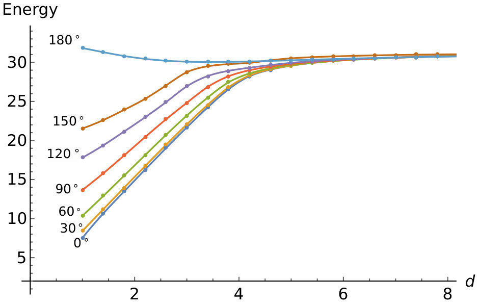 Figure 1
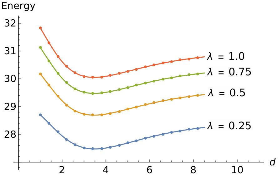 Figure 2
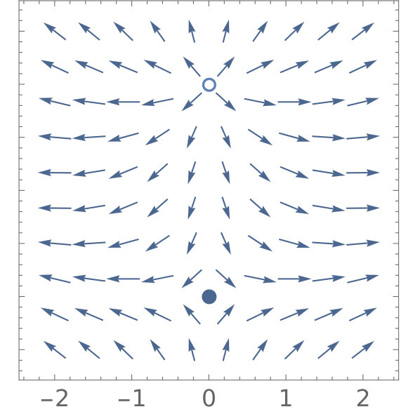 Figure 3
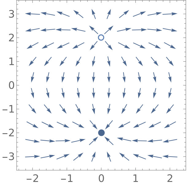 Figure 4
 Figure 5
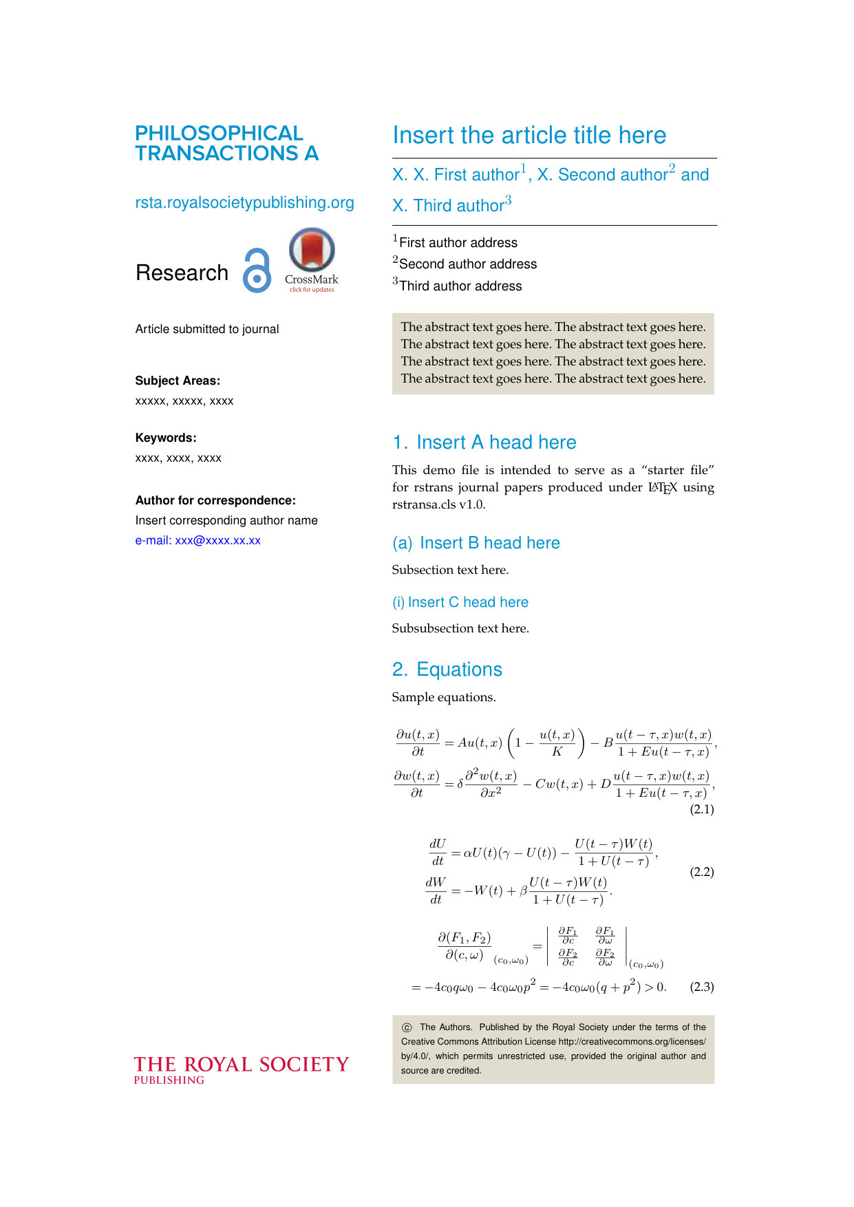 Figure 6
 Figure 7
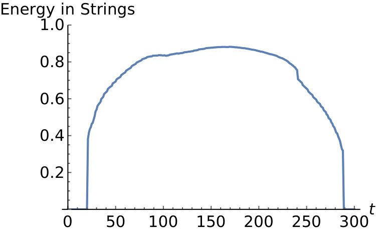 Figure 10
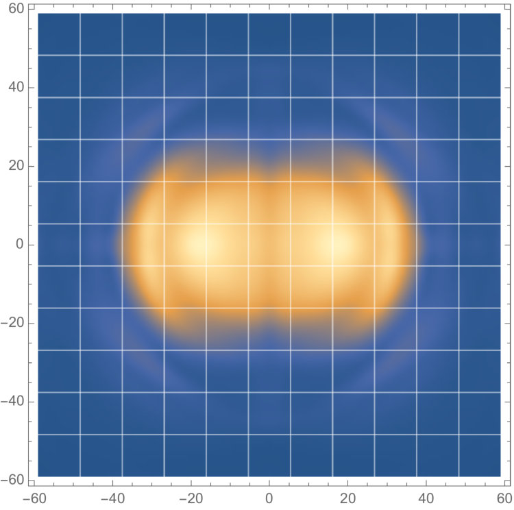 Figure 11
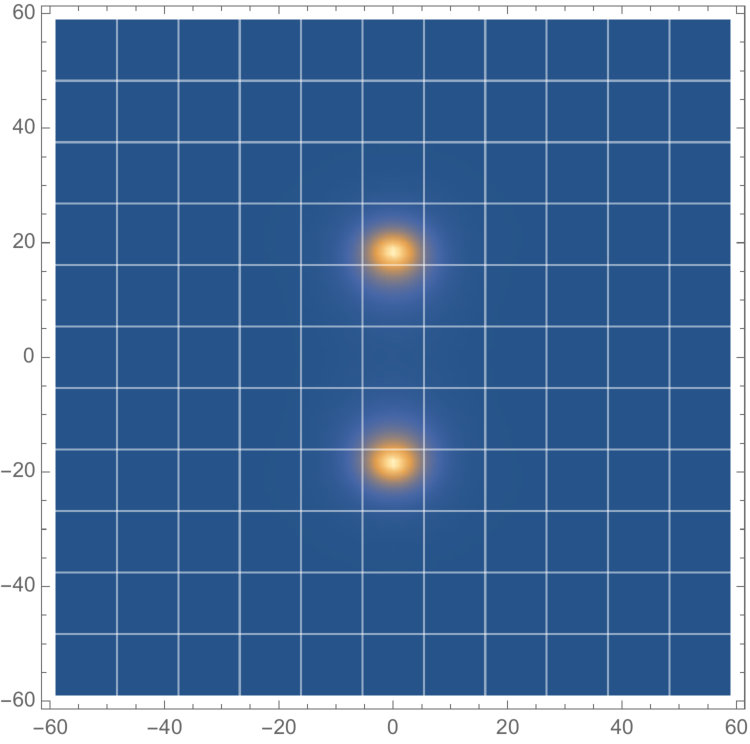 Figure 12
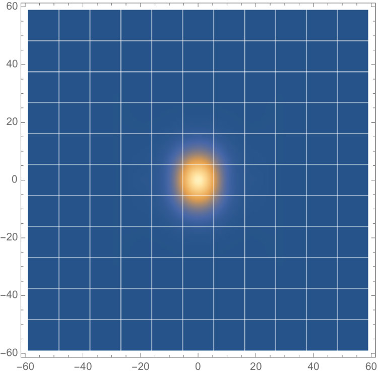 Figure 13
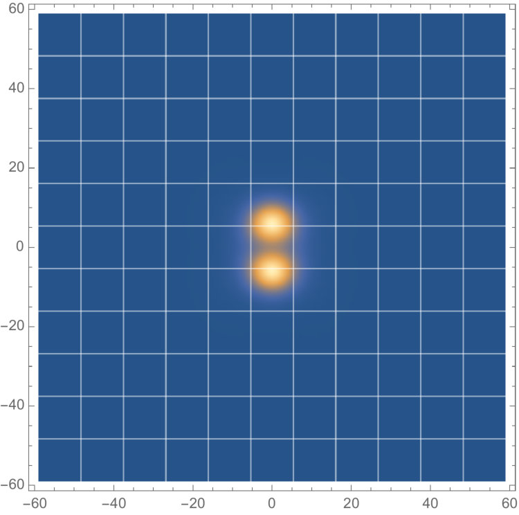 Figure 14
 Figure 15
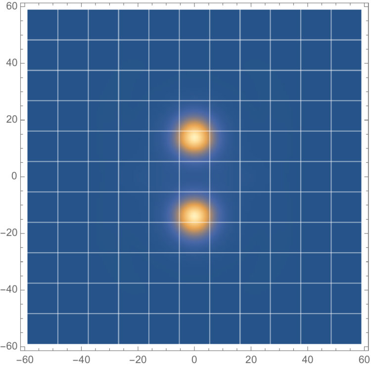 Figure 16
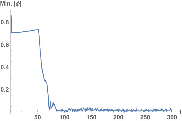 Figure 17
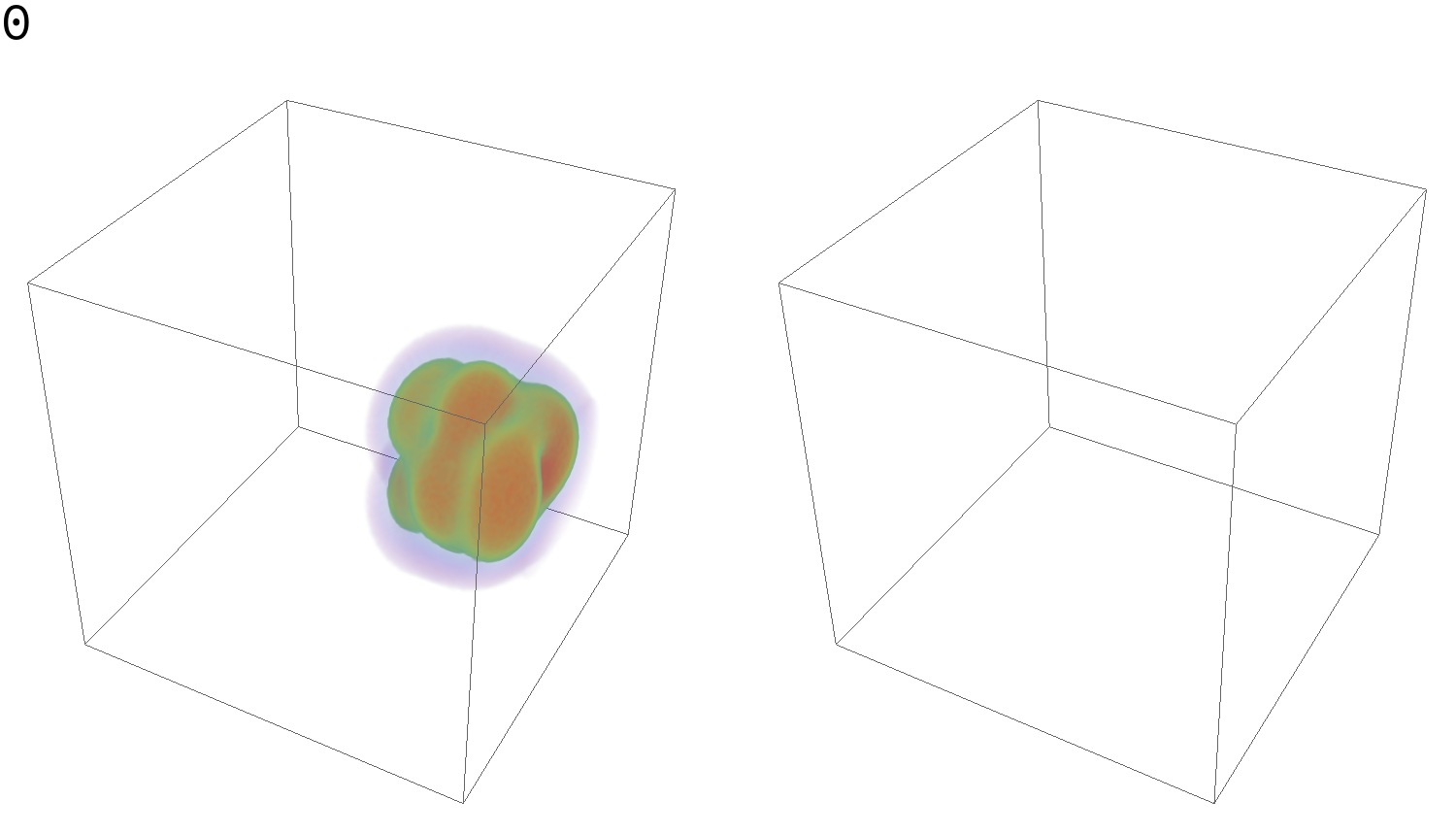 Figure 1
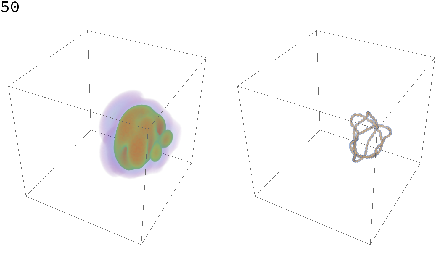 Figure 2
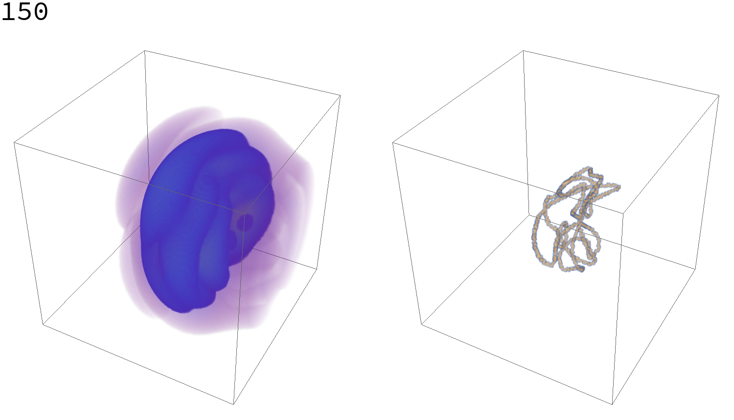 Figure 3
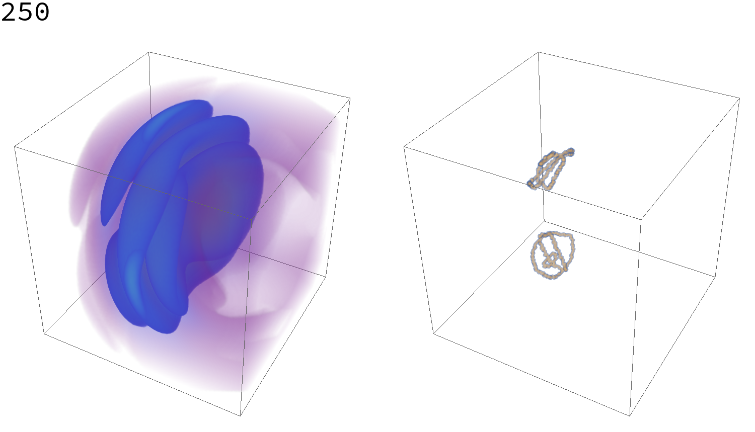 Figure 4
 Figure 5
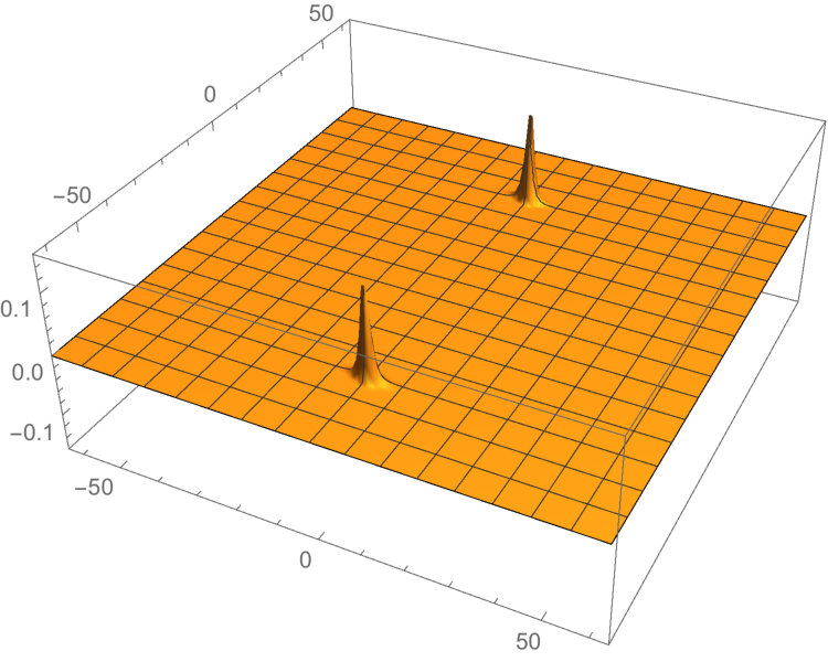 Figure 23
 Figure 24
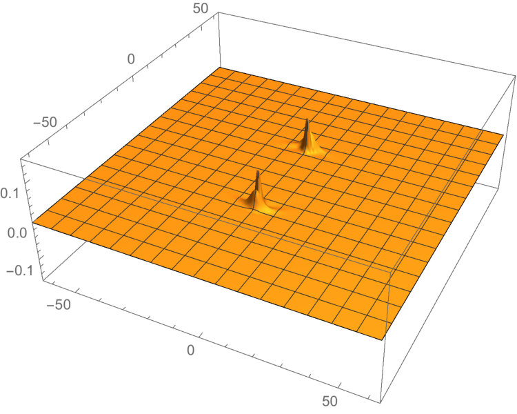 Figure 25
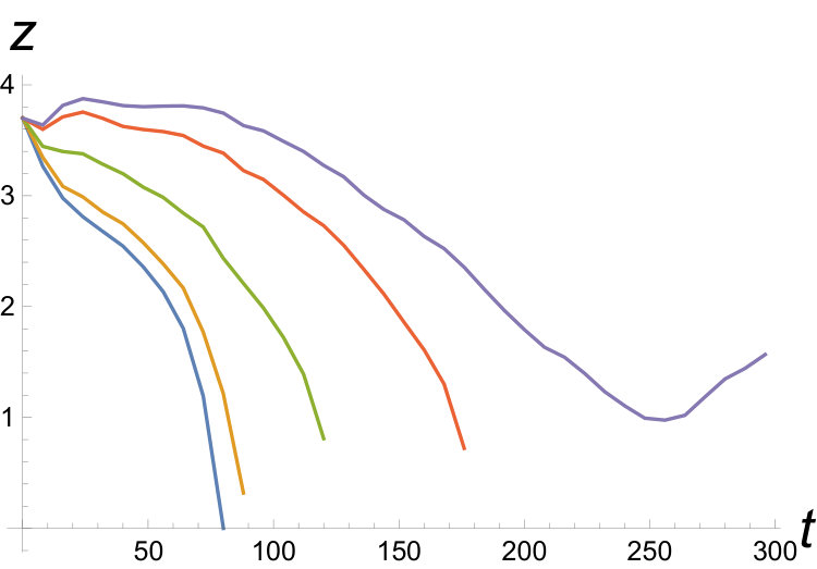 Figure 26
Peer Reviews
No public reviews on file for this paper yet. If you reviewed it on a platform where reviews are public (OpenReview, ICLR, NeurIPS, ICML), you can paste yours below so the community can read it here.
Videos
No videos yet. Explain this paper in a talk, walkthrough, or lecture? Add one.
\subject
field theory, particle physics
\corres
Insert corresponding author name
Monopole-antimonopole: interaction, scattering and creation
Ayush Saurabh
Tanmay Vachaspati
1Physics Department, Arizona State University, Tempe, AZ 85287, USA.
Abstract
The interaction of a magnetic monopole-antimonopole pair depends on their separation as well as on a second “twist” degree of freedom. This novel interaction leads to a non-trivial bound state solution known as a sphaleron and to scattering in which the monopole-antimonopole bounce off each other and do not annihilate. The twist degree of freedom also plays a role in numerical experiments in which gauge waves collide and create monopole-antimonopole pairs. Similar gauge wavepacket scatterings in the Abelian-Higgs model lead to the production of string loops that may be relevant to superconductors. Ongoing numerical experiments to study the production of electroweak sphalerons that result in changes in the Chern-Simons number, and hence baryon number, are also described but have not yet met with success.
keywords:
magnetic monopoles
1 Introduction
Magnetic monopoles have been known for over 40 years now as regular solutions in non-Abelian gauge theories [1, 2]. They provide a fertile playground for theoretical ideas [3] and are also relevant to physical considerations as they are necessarily present in all grand unified models [4]. In the standard model of the electroweak interactions, only confined magnetic monopoles exist. Even so, they can lead to insight into processes such as baryon number violation [5].
In the present work we are interested in properties of monopole-antimonopole ( ) pairs. How do monopoles interact with antimonopoles when they are at rest? How do they scatter? Can they be produced in scattering experiments? Can they play a role in particle physics? There is a large body of work on the first two questions and there are also several excellent texts [3, 6] where the reader can access results. Our recent work [7, 8, 9] provides numerical evidence for some of these works and extends them in some cases. The question of creation has also received attention but it is difficult to answer especially as it seems to require a description of a non-perturbative final state ( ) in terms of perturbative initial states (particles). The non-perturbative state is best described in classical terms (solutions of certain differential equations) while the perturbative state is best described in terms of quanta in a quantum field theory. Thus the process also requires a description that enables transition from quantum to classical variables. We shall largely bypass these deep questions and study the creation of when the initial state has large occupation number and can be described in classical terms. After all, the initial state is up to us to prepare and we are free to set it up as we wish.
There are two applications of the work on creation that are more immediate. The first is that just as we can consider the creation of , we can also consider the creation of string loops. Indeed we find initial conditions in the Abelian-Higgs model that lead to string creation. These strings are produced in loops that live for a short time and then collapse. In some regime of parameters, the Abelian-Higgs model also provides a description of superconductors, leading to the possibility of experimentally producing strings in superconductors. (This is similar to the production of string loops in He-3 by the bombardment of neutrons in an experiment that has already been done [10].) The second application of the work on creation is in the context of the electroweak model. Here monopoles are confined and a monopole is always connected to an antimonopole by a Z-string. If we are able to create a confined electroweak , it will re-annihilate just as the loops of string in the Abelian-Higgs model re-collapse. Further, if the electroweak annihilates after some specific dynamics, the electroweak Chern-Simons number can change and lead to baryon number violation. Thus a better understanding of the creation of monopoles may enable processes in which baryon (and/or lepton) number changes. However, ongoing numerical work on the production of electroweak has not yet resulted in a change of Chern-Simons number.
2 in SO(3) model
We consider an SO(3) gauge theory with a scalar in the adjoint representation with Lagrangian
[TABLE]
where , the covariant derivative is defined as,
[TABLE]
and the gauge field strength is given as
[TABLE]
The energy of a static field configuration is given by,
[TABLE]
It is known [1] that the model has a monopole solution
[TABLE]
where and are profile functions that can be found by solving the equations of motion with the boundary conditions
[TABLE]
The configuration can now be written by gluing together a monopole and an antimonopole. There is some freedom in this procedure but all we need is that the monopole and antimonopole be located with some fixed separation and that they should have a fixed relative twist. Then the fields can be relaxed to the lowest energy configuration subject to these constraints, and/or used as initial conditions for time evolution. We choose the scalar field orientations to be given by
[TABLE]
Note that the configuration has two free parameters. The separation of the monopole and antimonopole, , is hidden in the spherical angles and that are with respect to coordinate systems with origins at the monopole and antimonopole respectively. The second is the twist paramter . The scalar field configurations for are illustrated in Fig. 1. The expression for the scalar field with the profile functions included is
[TABLE]
where anad are the distances to the monopole and antimonopole respectively. For the gauge fields we take the configuration,
[TABLE]
2.1 Interaction
The starting configuration in Eq. (10) can now be relaxed so as to lower the field energy but with fixed values of and . A numerical scheme was implemented for this relaxation in Ref. [9] and the results are shown in Fig. 2. The energy depends on and . The most interesting feature is that the energy curve for has a minimum. The symmetry under then shows that the energy function has a saddle point at and (in units in which and the vector mass and the monopole radius are 1). Thus the SO(3) equations have a saddle point solution corresponding to a bound state of a monopole-antimonopole as was first shown to exist by Taubes in the SO(3) model in Ref. [11, 12] and also discovered in the electroweak model by Manton in Ref. [13].
2.2 Scattering
The initial conditions for a monopole-antimonopole pair were also evolved using the classical equations of motion in Ref. [8]. Fig. 3 shows snapshots of the scattering for an untwisted , while Fig. 4 shows the scattering when the are twisted (). In the untwisted case, the annihilate, while in the twisted case they come close but not close enough to annihilate. In fact, they bounce back as seen in Fig. 5.
2.3 Creation
Next we discuss the creation of . The issue is that monopoles are described as solutions to the classical equations of motion, while particles are quanta in a quantum field theory. So creation requires a description of magnetic monopoles in a quantum field theory. Further, a monopole is a non-perturbative solution since its magnetic charge is proportional to where is the gauge coupling. Perturbative calculations can only give a power law expansion in and cannot describe monopoles. Thus any attempt at a perturbative calculation of the creation amplitude is sure to fail.
We take a different approach to creation. We do not consider creation from the collision of just two (or few) particles. Instead we consider the collision of classical wavepackets of gauge particles. These classical wavepackets contain a large number of particles. With such initial conditions, it becomes possible to study creation because we can simply evolve the initial conditions using the classical equations of motion. However, even within this classical framework, it is not clear what initial conditions will lead to creation and it requires some physical intuition, guesswork and luck to find initial conditions that successfully produce monopoles.
If two wavepackets of gauge fields with sufficient energy collide, we can expect that a monopole-antimonopole pair can be created but this is not sufficient because we also require that the monopole and antimonopole separate from each other and do not re-annihilate. On the other hand, a monopole and an antimonopole attract each other by the Coulomb force and this will tend to bring them together, causing them to annihilate. However, if the are twisted, as discussed in the previous sections, the twist could provide a repulsive force between the monopole and antimonopole and may help separate them. This suggests that the initial gauge wavepackets carry some parity violating structure, which is possible if they are circularly polarized.
Some more intuition may be gained from a result in magneto-hydrodynamics (MHD), that the magnetic helicity is a conserved quantity. For our purposes, the magnetic helicity can be thought of as a measure arising due to twisted or helical magnetic field lines. Further, magnetic helicity likes to spread out. Therefore, if one provides initial conditions that compress magnetic helicity, the system will try and resist. But the only way out is to break the MHD approximation and one way for this to happen is by the creation of magnetic monopoles. So perhaps the compression of magnetic helicity can lead to creation.
After this guesswork, the following circularly polarized gauge wavepackets were used to construct the initial conditions:
[TABLE]
where the profile functions , and will be specified shortly. Note that this is not a solution to the field equations. It is simply a configuration that represents a gauge wavepackets that is moving in the direction. The configuration is complicated due to the requirement that the initial conditions need to satisfy the Gauss constraints. The chosen configuration satisfies , and the electric field satisfies the Gauss constraint with vanishing charge density. We will arrange for an initially vanishing charge density by setting when we choose initial conditions for the scalar field.
The profile functions are chosen to create localized packets in all directions
[TABLE]
[TABLE]
where is an amplitude and is a width. The frequencies and can be different in general but here we only consider . The case corresponds to scattering of left- and right-handed circular polarizations, while corresponds to scattering of left- on left-handed circular polarization waves.
Now we can state our initial conditions for the gauge field,
[TABLE]
For the scalar field we choose
[TABLE]
Next we need to evolve these initial conditions. The SO(3) equations of motion are written in a form inspired by Numerical Relativity that provides for numerical stability [14]. The field theory parameters in the numerical work are , , , and the initial condition parameters were chosen to be , , , , .
A first sign that monopoles are produced is that the evolution produces zeros of the Higgs field. In Fig. 6, the minimum value of over the entire simulation box is plotted as a function of time. The sharp drop after some time and the persistence of the zero value indicates that monopoles have been produced and survive until the end of the evolution.
Another characteristic of magnetic monopoles is that they are topological structures and so there is a topological charge density that should be non-vanishing at the location of the monopoles. The formula for the topological charge within a surface is given by,
[TABLE]
where . Fig. 7 shows three different slices of the simulation box at and at the end of the run. The plots show 4 positive peaks at and and 4 negative peaks at . Thus the run produces 4 monopoles and 4 antimonopoles.
These numerical experiments are proof of concept showing that a class of initial conditions can be constructed to create magnetic monopoles.
3 String Creation
Just as we considered the creation of , we can consider the creation of strings (vortices). The problem here is that only loops of strings can be created and these will be ephemeral as they will re-collapse and annihilate. On the other hand, vortices are present in superconductors and so some of these ideas can be implemented in the laboratory.
String solutions exist in the Abelian Higgs model that is given by the Lagrangian,
[TABLE]
where is a complex scalar field, , is the U(1) gauge field with field strength tensor , and and are coupling constants.
The solution for a straight string along the axis is,
[TABLE]
where we work in cylindrical coordinates , , and are profile functions that vanish at the origin and go to 1 asymptotically. The energy per unit length (also the tension) of the string is given by
[TABLE]
where . The function is known numerically and is a smooth, slowly varying function with , equals the vector mass, . For not too large, the thickness of the scalar fields in the string is and of the vector fields is . We will only consider .
The string is characterized by a topological winding number that is defined by
[TABLE]
where is the phase of the scalar field at a given point on the contour and denotes the parameter along the integration curve.
We based the initial conditions for our simulations on those used for monopole-antimonopole production in Sec. mmbarcreation with in the monopole case corresponding to in the string case. Now the initial conditions for the gauge fields and their time derivatives are,
[TABLE]
The initial conditions for the scalar field are “trivial”,
[TABLE]
With these initial conditions, we were able to explore the parameter space for the formation of U(1) gauge strings in two settings: (i) the prompt formation of strings from gauge fields and (ii) the formation of strings when gauge wavepackets collide. Here we only show the results of prompt string formation in which a single wavepacket of gauge fields evolves to produce strings as in Fig. 8.
Unlike the case of magnetic monopoles, the string loops that are formed are short-lived as they collapse and produce radiation as is evident from Fig. 9. The loops may live longer if we could find initial conditions that provide them with greater angular momentum but these too will radiate and dissipate. On the other hand, once a magnetic monopole and antimonopole pair are produced with sufficient velocity, they will move apart and survive indefinitely. Furthermore, magnetic monopoles are localized objects and so the colliding wavpackets need not be very extended. For strings, on the other hand, the wavepackets have to extend over a region that is the size of the string loop that is to be produced, and only relatively small loops can be produced. In these respects it appears that magnetic monopoles are easier to produce than strings.
The flip side is that we know systems that contain gauge strings while the existence of magnetic monopoles is still speculative. Gauge strings are known to exist in superconductors and, in that setting, our gauge field wavepackets correspond to photon wavepackets. This suggests that by shining light on superconductors we could produce strings within the superconductor. However, a realistic superconductor is described by a different set of equations that take into account the dependence of the model parameters on the temperature. It will be interesting to adapt our analysis to study string production in superconductors.
4 in Electroweak Model
The electroweak model is based on the symmetry breaking
[TABLE]
In this case, the initial symmetry group is not simply connected and it requires some care to see that there are no topological monopoles in the model. A simpler way to see the absence of topological magnetic monopoles is that the electroweak Higgs, , is an doublet
[TABLE]
and the minimum of the Higgs potential is given by
[TABLE]
where is the vacuum expectation value of the Higgs. Thus the vacuum manifold is a three-sphere that does not admit incontractible two-spheres that are necessary to obtain topological monopoles.
The absence of topology in the standard model still leaves room for confined magnetic monopoles. Indeed it was shown in Ref. [15, 16] that such magnetic monopoles do exist in the electroweak model. These electroweak monopoles carry magnetic charge but are attached to a string made of fields that connect the monopole to an antimonopole. The situation is very similar to that of a quark that carries electric charge but is confined by a QCD flux tube that connects it to an anti-quark of opposite electric charge.
Can we create electroweak monopole-antimonopole pairs by colliding gauge wavepackets? Even if we manage to create a monopole-antimonopole pair, they will be confined by the string that will pull them together and cause them to annihilate. So electroweak monopoles can at best be created temporarily, somewhat like the string loops we discussed in Sec. 3.
There is one situation which is of interest even if electroweak monopoles are produced and that then annihilate. This is if the monopoles are produced but then annihilate after they have twisted by . A signature of such an event will be a change in the Chern-Simons number which is defined as
[TABLE]
where are the gauge fields and the hypercharge gauge field. Changes in the Chern-Simons number are also indicative of baryon number violation in the electroweak model when fermions are included.
The initial conditions of Sec. 2.3 used to study monopole creation in the SO(3) model can be adapted to the electroweak model. Numerical experiments as of this time have not yielded a successful Chern-Simons number changing event but the search continues.
5 Conclusions
Magnetic monopoles are predicted in a wide class of particle physics models, e.g. all models of Grand Unification. Indeed, the realization that Grand Unification and standard cosmology predicts an over-abundance of magnetic monopoles led to the proposal of inflationary cosmology that vastly dilutes the monopole abundance. Thus monopoles are expected to be present in the physics that governs the universe but are not realized in our observable universe.
This peculiar circumstance is not special to magnetic monopoles. The underlying physics also admits other structures such as cars and computers but these do not occur naturally. Instead they require human intervention for their existence. Magnetic monopoles fall in this category – they may require humans to create them. Whether humans have the will to create monopoles is another question and the answer will hinge on their perceived utility. (One potential utility is to use magnetic monopoles for catalyzing proton decay and to harness the released energy.)
These considerations have led us to study the interactions and dynamics of magnetic monopole-antimonopole pairs. The interaction of is non-trivial because of a twist that was known to exist from the 70’s [11, 12]. We have described numerical work that confirms the picture and quantifies it more accurately. The twist also leads to non-trivial dynamics. The scattering of monopole-antimonopole can lead to a bounce instead of annihilation. We have used these results to intuit initial conditions that can lead to monopole creation and have successfully tested them to see the production of four monopoles and four antimonopoles. Similar studies that lead to the production of strings may be relevant to superconductors in the lab. When these methods are applied to the electroweak model, they can potentially generate Chern-Simons number changing events that lead to baryon number violation. However we have not yet seen such an event in our numerical experiments and are continuing our explorations.
\aucontribute
AS and TV developed the numerical code, performed the analysis and drafted the manuscript. All authors read and approved the manuscript.
\competing
The author(s) declare that they have no competing interests.
\funding
Insert funding text here.
\ack
AS and TV are supported by the U.S. Department of Energy, Office of High Energy Physics, under Award No. DE-SC0018330 at Arizona State University.
The reference list from the paper itself. Each links out to its DOI / PubMed record.
- 1[1] ’t Hooft G. 1974 Magnetic monopoles in unified gauge theories. Nuclear Physics B 79 , 276 – 284.
- 2[2] Polyakov AM. 1974 Particle Spectrum in the Quantum Field Theory. JETP Lett. 20 , 194–195. [Pisma Zh. Eksp. Teor. Fiz.20,430(1974)].
- 3[3] Rebbi C, Soliani G, editors. 1985 Solitons and Particles .
- 4[4] Preskill J. 1987 VORTICES AND MONOPOLES. In Architecture of Fundamental Interactions at Short Distances: Proceedings, Les Houches 44th Summer School of Theoretical Physics: Les Houches, France, July 1-August 8, 1985, pt 1 pp. 235–338.
- 5[5] Vachaspati T, Field GB. 1994 Electroweak string configurations with baryon number. Physical review letters 73 , 373.
- 6[6] Manton NS, Sutcliffe P. 2007 Topological solitons . Cambridge University Press.
- 7[7] Vachaspati T. 2016 a Creation of Magnetic Monopoles in Classical Scattering. Phys. Rev. Lett. 117 , 181601.
- 8[8] Vachaspati T. 2016 b Monopole-antimonopole scattering. Phys. Rev. D 93 , 045008.