Collective spinon spin wave in a magnetized U(1) spin liquid
Leon Balents, Oleg A. Starykh

TL;DR
This paper investigates how interactions and gauge fluctuations influence the spin dynamics in a 2D U(1) spin liquid, revealing a new collective mode and effects relevant for experimental probes like ESR and neutron scattering.
Contribution
It introduces the concept of a spinon spin wave arising from interactions and analyzes gauge fluctuation effects on the spin susceptibility in a U(1) spin liquid.
Findings
Discovery of a spinon spin wave mode splitting from the two-spinon continuum.
Gauge fluctuations induce a finite lifetime and power-law weight outside the continuum.
Resonance linewidth in ESR scales linearly with temperature and as B^{2/3} with magnetic field.
Abstract
We study the transverse dynamical spin susceptibility of the two dimensional U(1) spinon Fermi surface spin liquid in a small applied Zeeman field. We show that both short-range interactions, present in a generic Fermi liquid, as well as gauge fluctuations, characteristic of the U(1) spin liquid, qualitatively change the result based on the frequently assumed non-interacting spinon approximation. Short-range interaction leads to a new collective mode: a "spinon spin wave" which splits off from the two-spinon continuum at small momentum and disperses downward. Gauge fluctuations renormalize the susceptibility, providing non-zero power law weight in the region outside the spinon continuum and giving the spin wave a finite lifetime, which scales as momentum squared. We also study the effect of Dzyaloshinskii-Moriya anisotropy on the zero momentum susceptibility, which is measured in…
Click any figure to enlarge with its caption.
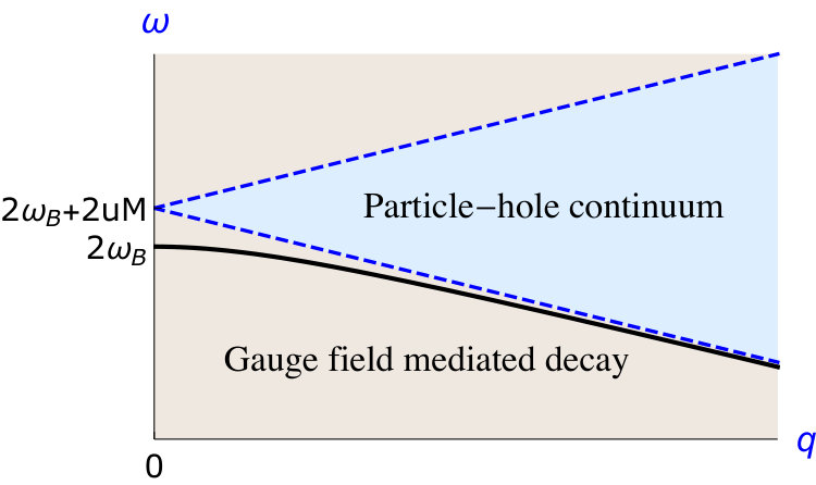 Figure 1
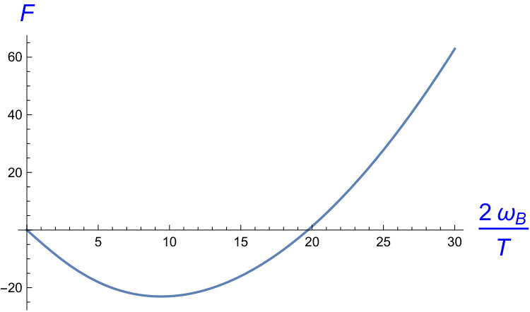 Figure 2
Peer Reviews
No public reviews on file for this paper yet. If you reviewed it on a platform where reviews are public (OpenReview, ICLR, NeurIPS, ICML), you can paste yours below so the community can read it here.
Videos
No videos yet. Explain this paper in a talk, walkthrough, or lecture? Add one.
Collective spinon spin wave in a magnetized U(1) spin liquid
Leon Balents
Kavli Institute for Theoretical Physics, University of California, Santa Barbara, CA 93106, USA
Oleg A. Starykh
Department of Physics and Astronomy, University of Utah, Salt Lake City, Utah 84112, USA
Abstract
We study the transverse dynamical spin susceptibility of the two dimensional U(1) spinon Fermi surface spin liquid in a small applied Zeeman field. We show that both short-range interactions, present in a generic Fermi liquid, as well as gauge fluctuations, characteristic of the U(1) spin liquid, qualitatively change the result based on the frequently assumed non-interacting spinon approximation. The short-range part of the interaction leads to a new collective mode: a “spinon spin wave” which splits off from the two-spinon continuum at small momentum and disperses downward. Gauge fluctuations renormalize the susceptibility, providing non-zero power law weight in the region outside the spinon continuum and giving the spin wave a finite lifetime, which scales as momentum squared. We also study the effect of Dzyaloshinskii-Moriya anisotropy on the zero momentum susceptibility, which is measured in electron spin resonance (ESR), and obtain a resonance linewidth linear in temperature and varying as with magnetic field at low temperature. Our results form the basis for a theory of inelastic neutrons scattering, ESR, and resonant inelastic x-ray scattering (RIXS) studies of this quantum spin liquid state.
The search for the enigmatic spin liquid state has switched into high gear in recent years. Dramatic theoretical (Kitaev model Kitaev (2006); Savary and Balents (2017) and spin liquid in triangular lattice antiferromagnet Zhu and White (2015)) and experimental (YbMgGaO4 Paddison et al. (2017); Shen et al. (2018) and -RuCl3 Banerjee et al. (2016)) developments leave no doubt of the eventual success of this enterprise. To push this to the next stage, it is incumbent upon the community to identify specific experimental signatures that evince the unique aspects of these states. In this paper, we focus on the two dimensional quantum spin liquid (QSL) with a spinon Fermi surface. This is a priori the most exotic two dimensional QSL state, and yet one which has repeatedly been advocated for in both theory Ioffe and Larkin (1989); Motrunich (2005); Lee and Lee (2005); Motrunich (2006); Nave and Lee (2007) and experiment Yamashita et al. (2008); Shen et al. (2016); Fåk et al. (2017); Shen et al. (2018). Specifically, we study the dynamical susceptibility of the -component of the spin operator
[TABLE]
which is an extremely information-rich quantity, and is accessible through inelastic neutron scattering Banerjee et al. (2017), ESR Smirnov et al. (2015); Ponomaryov et al. (2017), and RIXS Halász et al. (2016). The fractionalization of triplet excitations into pairs of spinons is a fundamental aspect of a QSL, and is expected to manifest in as two-particle continuum spectral weight Norman (2016); Savary and Balents (2017); Zhou et al. (2017), a surprising feature which appears more characteristic of a weakly correlated metal than a strongly correlated Mott insulator.
In a mean-field treatment in which the spinons are approximated as non-interacting fermions, this continuum has a characteristic shape at small frequency and wavevector in the presence of an applied Zeeman magnetic field, as discussed in Li and Chen (2017). In particular, there is non-zero spectral weight in a wedge-shaped region which terminates at a single point along the energy axis at zero momentum. Our analysis reveals the full structure in this regime beyond the mean field approximation. Notably, we find that interactions between spinons qualitatively modify the result from the mean-field form, introducing a new collective mode – a “spinon spin wave” – and modifying the spectral weight significantly.
We recapitulate the derivation of the theory of the spinon Fermi surface phase Nagaosa (1999); Lee et al. (2006). One introduces Abrikosov fermions by rewriting the spin operator , where are canonical fermionic spinors on site with spin-1/2 index (repeated spin indices are summed). This is a faithful representation provided the constraint is imposed – this constraint induces a gauge symmetry. In a path integral representation, the constraint is enforced by a Lagrange multiplier , which takes the role of the time-component of a gauge field, i.e. scalar potential. Microscopic exchange interactions, which are quadratic in spins, and are therefore quartic in fermions, are decoupled to introduce new link fields whose phases act as the spatial components of the corresponding gauge fields , i.e. the vector potential.
To describe the universal low energy physics, it is appropriate to consider “coarse-grained” fields descending from the microscopic ones, and include the symmetry-allowed Maxwell terms for the U(1) gauge field. Furthermore, due to the finite density of states at the spinon Fermi surface, the longitudinal scalar potential is screened and the time component can then be integrated out to mediate a short-range repulsive interaction between like charges. Therefore we consider the Euclidean action , where Kim et al. (1994); Nagaosa (1999); Lee et al. (2006)
[TABLE]
Here is the space-time coordinate, is the three-momentum, is a two-component spinor, with spin indices that are suppressed when possible, describes static magnetic field and includes the g-factor as well as the Bohr magneton. The gauge dynamics is derived in the Coulomb gauge with . The gauge action is generated by spinons and and represent Landau damping and diamagnetic susceptibility of non-interacting spinon gas, correspondingly ( is the spinon mass, is the spinon density and is the Fermi momentum of non-magnetized system).
We proceed with the assumption of SU(2) symmetry, a good first approximation for many spin liquid materials, and address the effect of its violations in the latter part of the paper. Previous investigations focused on the transverse vector potential , which is not screened but Landau damped, and hence induces exotic non-Fermi-liquid physics. For example, one finds a self-energy varying with frequency as , and a singular contribution to the specific heat Nagaosa (1999); Lee et al. (2006). However, notably, the transverse gauge field has negligible effects on the hydrodynamic long-wavelength collective response Kim et al. (1994). Here, we instead focus on the short-range repulsion , which produces an exchange field that dramatically alters the behavior in the presence of an external Zeeman magnetic field giving rise to finite magnetization. Gauge fluctuations play a subsidiary role which we also include.
An important constraint follows purely from symmetry. Provided the Hamiltonian in zero magnetic field has SU(2) symmetry, a Zeeman magnetic field leads to a fully determined structure factor at zero momentum. Specifically, the Larmor/Kohn theorem Oshikawa and Affleck (2002) dictates that the only response at , , where is the magnetization and is the spinon Zeeman energy. For free fermions, the delta function is precisely at the corner of the spinon particle-hole continuum (also known as the two-spinon continuum). However, the contact exchange interaction shifts up the particle-hole continuum, at small momentum , away from the Zeeman energy to . This is seen by the trivial Hartree self-energy
[TABLE]
where we use a zig-zag line to diagrammatically represent the local interaction, and , and is the expectation value of spin- spinon density in the presence of magnetic field. Consequently, for the Larmor theorem to be obeyed, there must be a collective transverse spin mode at small momenta.
This collective spin mode is most conveniently described by the Random Phase Approximation (RPA), which corresponds to a standard resummation of particle-hole ladder diagrams Aronov (1977). For the particular case of a momentum-independent contact interaction, one has
[TABLE]
where the fermion lines correspond to the spinon Green’s functions including the Hartree shift (3), and in this approximation is the bare susceptibility bubble, calculated using these functions. We will however use the second line in Eq. (Collective spinon spin wave in a magnetized U(1) spin liquid) to later define the RPA approximation even when gauge field corrections (but not the local interaction ) are included in . For the moment, we simply evaluate the bare susceptibility,
[TABLE]
Here are bosonic and fermionic Matsubara frequencies, respectively. A simple calculation, followed by analytical continuation , gives
[TABLE]
where square-roots are defined when their arguments are positive. The real/imaginary spin susceptibility describes domains outside/inside two-spinon continuum in the plane, Fig.1, correspondingly. At
[TABLE]
and therefore : the position of the two-spinon continuum is renormalized by the interaction shift. However, inserting (7) in the RPA formula (Collective spinon spin wave in a magnetized U(1) spin liquid) one finds that the RPA successfully recovers Larmor theorem at zero momentum for the interacting -invariant system,
[TABLE]
Therefore the contribution at is solely from the collective mode, with no spectral weight from the continuum at . Dispersion of the collective spin mode is obtained with the help of (Collective spinon spin wave in a magnetized U(1) spin liquid) and ,
[TABLE]
For small the collective mode is dispersing downward quadratically , while in the opposite limit it approaches the low boundary of the spinon continuum, . Retaining quadratic in terms in (5) will lead to the termination of the collective mode at some at which the spin wave enters the two-spinon continuum.
This physics is not unique to spin liquids but applies to paramagnetic metals. Historically, this spin wave mode was predicted by Silin in 1958 for non-ferromagnetic metals within Landau Fermi liquid theory Silin (1958, 1959); Platzman and Wolff (1967); Leggett (1970), and observed via conduction electron spin resonance (CESR) in 1967 Schultz and Dunifer (1967). At the time, this observation was considered to be one of the first proofs of the validity of the Landau theory of Fermi-liquids Platzman and Wolff (1973). Unlike the more well-known zero sound Abel et al. (1966), an external magnetic field is required in order to shift the particle-hole continuum up along the energy axis to allow for the undamped collective spin wave to appear outside the particle-hole continuum, in the triangle-shaped window below it. Second order in the interaction corrections (beyond the ladder series) do cause damping of this spin mode Meyerovich and Musaelian (1994); Golosov and Ruckenstein (1995); Zyuzin et al. (2018).
However, in the spin liquid, there is an additional branch of low energy excitations due to the gauge field , dispersing as . The very flat dispersion of the gauge excitations suggests it may act as a momentum sink, so that, for example, an excitation consisting of a particle-hole pair plus a gauge quantum may exist in the “forbidden” region where the bare particle-hole continuum vanishes and the collective spin mode lives. It is therefore critical to understand the effect of the gauge interactions upon the dynamical susceptibility. To this end, we consider the dressing of the particle-hole bubble by gauge propagators. Guided by the above thinking, we expect that it is sufficient to consider all diagrams with a single gauge propagator (denoted by wavy line).
[TABLE]
Calculations described in SM lead to
[TABLE]
That is, the dressed susceptibility has a non-zero imaginary part in the previously kinematically forbidden region outside the spinon particle-hole continuum, see Fig.1. This is a new continuum weight. However, the weight in this new continuum contribution vanishes quadratically in momentum as is approached. This is an important check on the calculations, since the Larmor theorem still applies to the full theory (Collective spinon spin wave in a magnetized U(1) spin liquid) with the gauge field, which implies that precisely at zero momentum, there can be no new contributions. Similar to Kim et al. Kim et al. (1994), who considered diagrams for the density correlations and optical conductivity, this result relies on important cancellations between self energy (first two diagrams) and vertex corrections (last diagram), which are needed to obtain this proper behavior of .
Within the RPA approximation of Eq. (Collective spinon spin wave in a magnetized U(1) spin liquid), but now with , we see that the dependence of is sufficient to ensure that the width (in energy) of the collective spin mode becomes narrow compared to its frequency at small momentum: this is the standard criteria for sharpness and observability of a collective excitation. The real part of , derived in Eq. (S53), modifies the dispersion of the collective mode too, but preserves its downward character within the approximationSM . The final result for the dynamical susceptibility is summarized in Fig. 1. Away from the zero momentum axis is always non-zero, and is the sum of several distinct contributions. Inside this spinon-gauge continuum, the spinon spin wave appears as a resonance which is asymptotically sharp at small momentum. We note that, while our calculations are done in two dimensions, a spinon spin wave with the same qualitative features is also present in the three dimensional U(1) QSL.
For observation of the spinon spin wave via inelastic neutron or RIXS experiment, the mode should be present over a range of momenta which is not too narrow. Because the extent of the ‘decay-free” triangular shaped region in Fig.1 is determined by , this requires that the Zeeman energy should be a substantial fraction of the exchange integral (effective Fermi energy). This makes spin liquid materials with of order 10 K ideal candidates for observation, in constrast with usual metals for which is vanishingly small.
The above results apply to the case in which SU(2) spin rotation symmetry is broken only by the applied Zeeman field. Breaking of the SU(2) invariance by anisotropies invalidates the Larmor theorem and causes a shift and more importantly a broadening of the spin collective mode even at zero momentum Maiti and Maslov (2015). This is of particular importance for electron spin resonance, which has high energy resolution but measures directly at zero momentum only Oshikawa and Affleck (2002). The way in which the resonance is broadened depends in detail on the nature of the anisotropy, the orientation of the applied magnetic field, etc., so it is not possible to give a single general result. Instead, we provide one example of this physics and consider the influence of a Dzyaloshinskii-Moriya (DM) interaction, which is typically the dominant form of anisotropy for weakly spin-orbit coupled systems, provided it is symmetry allowed by the lattice. See for example Smith et al. (2003); Winter et al. (2017).
Guided by the arguments of symmetry and simplicity we next suppose that when projected to the spin liquid ground state manifold of the two-dimensional spin model, the DM interaction appears as a familiar spin-orbit interaction of the Rashba kind. A momentum-dependent spin splitting, of which this is the simplest example, is expected to appear in a model without spatial inversion symmetry because in the spinon Fermi surface state the spinons transform under lattice point group symmetries in the same way as usual electrons Iaconis et al. (2018). Then the term in the Hamiltonian breaking SU(2) spin invariance, , reads
[TABLE]
Here is the i-th component of the momentum operator, and is the strength of the Rashba coupling. The dependence on the minimal combination is required by the gauge invariance of the action in Eq. (Collective spinon spin wave in a magnetized U(1) spin liquid). Note that the magnetic field continues to couple to .
In the fixed Coulomb gauge, the momentum and gauge terms within the Rashba anisotropy of Eq. (12) have distinct effects. The former, momentum term, may be considered at the mean field level, as an intrinsic spin splitting in the spinon dispersion. Taking this into account, the ESR signal arises from vertical inter-band transitions Glenn et al. (2012). The variation of these transitions with momentum leads to an intrinsic lineshape, from which useful information about van Hove and other special points of the spinon bands may be extracted by a detailed analysisLuo et al. (2018). In Fermi liquids, this physics is responsible for chiral spin resonance Shekhter et al. (2005); Farid and Mishchenko (2006). In one dimensional spin chains with uniform DM interaction, the same basic physics leads to a splitting of the ESR line into a doublet Povarov et al. (2011).
The gauge field part of Eq. (12) consists mathematically of coupling of to the spin-non-conserving bilinear operators of spinons:
[TABLE]
where . This term has no simple mean field description, and is responsible for the magnetic field and temperature dependence of the dynamical spin susceptibility, and in particular the ESR line width .
Instead of a technically-involved diagrammatic calculation (which is also possible and confirms the results otherwise obtained) we employ an elegant short-cut which is based on the modern reincarnation Oshikawa and Affleck (2002); Furuya (2017) of the classic ESR formulation by Mori and Kawasaki Mori and Kawasaki (1962). We are interested in the retarded Green’s function of the transverse spin fluctuations , which defines the zero momentum self-energy . The ESR theory shows (see SM ) that this self-energy is related to the correlations of the perturbation operator , according to
[TABLE]
Eq. (14) directly expresses the ESR linewidth in terms of the retarded Green’s function of the perturbing operator . Observe that and hence to the second order in the spin-orbit coupling, Eq. (14) may be calculated with respect to the isotropic Hamiltonian of the ideal spin liquid subject to the Zeeman magnetic field .
For the Rashba coupling, one obtains , so that the calculation of reduces to a convolution-type integral over energy and momentum of the spectral functions of the spinon magnetization density and the gauge field . This instructive calculation is described in SM and results in the full scaling function prediction for the ESR linewidth
[TABLE]
The scaling function is plotted in Figure 2 and is characterized by these limits: and . Consequently, in the low-temperature limit the linewidth follows a ‘fractional’ scaling with the magnetic field, . Also notable is the non-monotonic dependence of the scaling function on its argument. The full scaling function represents a non-trivial quantitative prediction for the the present model of magnetic anisotropy.
However, while all isotropic magnets are alike, all anisotropic magnets are anisotropic in their own way. We leave an exhaustive study of different mechanisms of anisotropy on ESR in spin liquids for future work.
Acknowledgements.
We thank A. Furusaki, D. Golosov, E. Mishchenko, D. Maslov and M. Raikh for discussions. Our work is supported by the NSF CMMT program under Grants No. DMR1818533 (L.B.) and DMR1928919 (O.A.S.), and we benefitted from the facilities of the KITP, NSF grant PHY1748958.
A Gauge field corrections to the transverse spin susceptibility
In the main text, we show that coupling to the gauge field induces spectral weight outside the region of the particle-hole continuum of the free fermion theory. On physical grounds, this is expected because in addition to the fermionic “quasiparticles” (we use quotes because they are not gauge invariant and have a non-Fermi liquid self-energy) the system possesses collective gauge excitations with a very soft dispersion relation . By creating a particle-hole pair and a photon, one may shunt enough of the total momentum of the excitation in to the photon to bring the remainder into the kinematically allowed region for particle-hole pairs, and because the energy of the photon is so small, this should be possible at just about any energy. With this picture in mind, we seek contributions to the dynamical spin structure factor with a single gauge field propagator, because “cutting” this line corresponds to a single excited photon excitation. With a single gauge propagator, there are three diagrams, as shown in Eq.(10). In the first and second contributions, and , the gauge line does not cross the particle-hole bubble, so the gauge field acts here as a self-energy correction to one of the two fermion lines. In the third diagram, the gauge line crosses the bubble, which represents a vertex correction. Care must be taken to combine all three terms because, as shown by Kim et al.Kim et al. (1994), there are important cancellations between them which are required to maintain gauge invariance and avoid unphysical results at low frequency and momentum.
The formal expressions for these three contributions are
[TABLE]
where we introduced bold face for spatial vectors, and as Matsubara frequencies, and the notation . The gauge propagator is
[TABLE]
with
[TABLE]
Here in a strict expansion the coefficient, which reflects Landau damping, itself originates from a fermion bubble. We will treat it however as just a bare kinetic term for the gauge field, following numerous previous works.
Consider the first two diagrams. In their expressions, the integral over defines the self-energy , and these terms can be rewritten in terms of . Specifically,
[TABLE]
where the self-energy is
[TABLE]
The self-energy is a standard calculation in the spinon gauge theory. Writing the Green’s function explicitly, we have
[TABLE]
with
[TABLE]
with and , and . Owing to the singular nature of the gauge propagator, the integral for the self-energy is dominated by small . Choosing coordinates , we have
[TABLE]
Here includes a spin-dependent Zeeman shift and a Hartree correction, which are both constant. From this form we expect the scaling , which means that is approximately normal to . This means we can replace by inside the gauge propagator, and that , for momentum near the Fermi surface. Consequently, we have
[TABLE]
The integral over can be done immediately – there is a small subtlety in the real part of the integral is conditionally convergent and dependent upon the cutoff, but this is anyway absorbed in a simple Fermi energy shift and can be set to zero. The imaginary part is well-defined and we obtain
[TABLE]
Note that the dependence on momentum has dropped out, so the self-energy is purely frequency dependent – what is called a “local” self-energy. The actual function can be calculated by performing the integration first: the regions at large positive and negative frequency cancel one another and the full result is just obtained from the integral between and . We find
[TABLE]
Then carrying out the integration gives finally
[TABLE]
The 2/3 power law dependence on frequency of the self-energy is a famous result for the spinon Fermi surface. Now we will rewrite Eqs. (A) in a form more amenable to seeing the partial cancellations of the three diagrams. To do so, we use the partial fractions rewriting
[TABLE]
which is straightforward to show using of the explicit forms for the Green’s functions. Using these forms, we obtain the sum of the two self-energy contributions as
[TABLE]
We aim to massage the susceptibility corrections into a form which exposes the small dependence more clearly and makes physical interpretation easier. First we split (A) into two distinct parts,
[TABLE]
with
[TABLE]
We show below that does not contribute to the imaginary part of the susceptibility and for a moment just neglect it. Next we use the identity
[TABLE]
to write
[TABLE]
Next we use the expression for the self-energy, (A), and obtain
[TABLE]
Similar manipulations of the vertex diagram give
[TABLE]
B Imaginary part
Let us consider the imaginary part of the (real frequency) susceptibility outside the particle hole (PH) continuum. This means that the explicit denominators in Eqs. (S20,S21) can be trivially analytically continued and considered purely real. We will however have to do the and integrals.
Start with (S20) and observe that if the product of the two square brackets is multiplied out, two of the four resulting terms, those involving the integral of and , do not have imaginary part outside the PH continuum simply because the integral over gives a result which is -independent (in the first of these we can make a shift and then integrate over ). That is, the only source of the imaginary part in these contributions is provided by the denominator in – and its imaginary part is restricted to the non-interacting PH continuum. The same argument actually applies to in (S17), one just needs to shift in the 2nd term on the right hand side there.
The two terms in that contribute outside the PH continuum are therefore given by
[TABLE]
Since the gauge propagator (S3) is even in , we can transform , followed by , in the first term in the square brackets above to obtain
[TABLE]
Now insert the spectral representation,
[TABLE]
Here we want
[TABLE]
In the usual way, we extract the spectral function via
[TABLE]
Eq.(S23) factorizes into
[TABLE]
where
[TABLE]
Carrying out the contour integrations we obtain
[TABLE]
Now we can analytically continue , with , and obtain the imaginary part, which constraints and collapses the -integration
[TABLE]
We observe that the second set of step-functions in (S29) is always zero for .
Now consider the vertex part, Eq. (S21). Expanding the product in the second line, we seek terms that have some dependence. There are just two such parts
[TABLE]
We again observe that the set of transformations , followed by , make the 2nd term in the square brackets above equal to the 1st, so that
[TABLE]
Evidently it reduces to a form very similar to (S27). Namely,
[TABLE]
Therefore, the imaginary part of is determined by the imaginary part of (S30),
[TABLE]
At this point, we can see that the quantity in the square brackets in Eq. (S34) vanishes at . Hence we may expect a quadratic dependence on (although this quantity has linear terms in , they vanish on integration or pair off with another linear part from ).
Let us see how to make the integration explicit. We choose polar coordinates according to
[TABLE]
We assume . The vector vertices in (S34) can be simplified as follows:
[TABLE]
At this point we need to compare and . From we deduce that . Therefore can be neglected in comparison with the two first terms and, moreover, . Hence (S36) reduces to just .
At the same time we see that . Therefore all vertices in (S34) can be safely approximated by . This strongly simplifies (S34),
[TABLE]
Next we observe that . This combination appears when combining denominators in the squared factor in Eq. (S37), and explicitly demonstrates the dependence of the result.
Next we can write
[TABLE]
The sign constraints on the energy in (S30) therefore are
[TABLE]
The frequency argument of the photon spectral function is
[TABLE]
Eq.(S41) shows that is bounded by from above, . At the same time . Let us use Eq. (S42) as a definition to trade the integration for one over . We have . In particular we see that
[TABLE]
Introduce
[TABLE]
so that .
Hence the second line in Eq. (S41) becomes while the first line just reads . Hence we obtain
[TABLE]
Now we can express all the energies in these variables.
[TABLE]
Putting everything together and using and (S26) for , we obtain for (S37)
[TABLE]
Now we can finally complete the evaluation. We integrate over first, using , and obtain that . Then we obtain the final result
[TABLE]
The characteristic scaling is now explicitly shown.
C Real part
The calculations of the real part are more difficult. In accordance with the common wisdom, see for example Chap.37 in the book by Abrikosov, Gor’kov, Dzyaloshinskii, the outcome depends on the order of the integration over Matsubara frequencies and momenta . Generally the first integrals carried out can be calculated simply and exactly in the absence of any ultraviolet cut-off. For a zero temperature quantum system, there is indeed no frequency cut-off, so integrating over all frequencies is correct. Integrating over all momenta is often not correct, because there is some lattice or bandwidth scale. Nevertheless, it can be tempting and simpler to try. In our case, carrying out the momentum integration first, similar to the procedure used by Kim et al.Kim et al. (1994), gives the incorrect result
[TABLE]
which holds in the limit . Importantly, the “result” is seemingly independent of a momentum cut-off even though the intermediate steps do require an explicit cut-off of the order when integrating over gauge momentum .
Carrying out the frequency integration first, similar to the calculations in Maslov et al. Zyuzin et al. (2018), produces quite a different answer
[TABLE]
Here is a high-momentum cut-off. Observe that diverges in the limit, which represents the static limit of gauge fluctuations, see (S3).
The technicalities of integrations leading to Eq. (S53) are tedious and require a number of simplifications performed at the proper stages in the calculation. These steps are carried out in the Mathematica Notebook “realchi1.nb” which is included in the Supplementary Materials, see the following link https://journals.aps.org/prb/supplemental/10.1103/PhysRevB.101.020401 . There we find that the most divergent part of the is given by
[TABLE]
We rescale by pulling out from the denominator, introducing and letting . Then
[TABLE]
where is the dimensionless upper cut-off of the momentum integration. We observe that for large integration variable is large as well, and therefore the -integral is approximated as . This gives us the quoted result, Eq.(S53).
In addition to the leading term in (S53), our calculation also produces a finite zero momentum independent contribution, which represents a correction to the magnetization
[TABLE]
Note that the prefactor is a simple pole, which reflects the Larmor theorem. Here is a momentum integral, which we calculate numerically. It parametrically depends on its argument . For example, for we obtain . Note that (S56) represents a quantum correction to (and hence the uniform susceptibility itself since is proportional to the appleid field), and vanishes in the limit . Interestingly, this correction comes from the real part of , (1), and is entirely absent when one integrates over the momenta before integrating over the frequencies.
We conclude by noting that imaginary part of , (S51), is not sensitive to the order of integrations discussed here. Carrying out calculations following Kim et al. (1994) and doing the momentum integration before the frequency one precisely reproduces Eq. (S51) (we do not show those redundant calculations here).
D RPA form
In the RPA approximation
[TABLE]
so that after the continuation to real frequency we obtain for the imaginary part of the susceptibility outside the non-interacting particle-hole continuum
[TABLE]
Damping of the collective spin mode is determined by (S51), since in this frequency range, while its dispersion is given by
[TABLE]
Considering (S53) as a small correction to the dispersion of the collective mode, which is justified by the expansion assumption of the gauge theory Kim et al. (1994), we parameterize the dispersion as and solve (S59) for by iterations. We find that the effective mass increases,
[TABLE]
and the dispersion of the collective mode flattens, correspondingly. But it retains its character.
E ESR in the U(1) Fermi surface spin liquid
E.1 Mori-Kawasaki formula
In the following we use Mori-Kawasaki (MK) formula, as derived in the Appendix of Oshikawa and Affleck (2002). A calculation with Matsubara Green’s functions is also possible, and was in fact carried out – the end structure of result is the same in the two approaches. This Matsubara calculation is instructive for understanding which diagrams contribute to the result. It shows that the ESR response is determined, in the leading order, only by the diagrams with self-energy insertions inside the spinon bubble. The vertex diagram is not present in that order. However, the calculation at finite temperature requires an analytical continuation to real frequency which is not an easy task. The MK approach is formulated directly in terms of retarded Green’s functions which is more convenient.
Let us parameterize , where the first term is SU(2) invariant, the second contains symmetry-breaking perturbations and the third describes interaction with static external field . The total spin of the system obeys the equations of motion
[TABLE]
where .
Then for the retarded Green’s function one obtains, using the identity and integration by parts,
[TABLE]
Repeating these steps for one finds
[TABLE]
Assuming next that and expanding to second order in the perturbation , we obtain explicit the expression for the self-energy
[TABLE]
The real part of this determines the shift of the resonance frequency from the ideal value, while the imaginary part determines all-important linewidth, resulting in Eq. (14) of the main text. Note that the first term in Eq. (S64) proportional to the commutator is frequency independent and hence does not contribute to the imaginary part, because the latter must be odd in frequency (as shown by the spectral representation).
Direct calculation gives the result shown in the main text
[TABLE]
This is a composite operator consisting of a convolution in momentum space of and the gauge field , .
E.2 Convolution formula
Since , the retarded Green’s function of the composite operator can be approximated by multiplied by the simple convolution of independent Green’s functions of and . This well known result is worked out below as follows.
Let , where and stand for two arbitrary independent (commuting) operators, . Then
[TABLE]
where the greater and lesser Green’s functions are defined by
[TABLE]
Note that here the lower index of the operators denotes time dependence, .
Using this representation and commutativity of and it is easy to show that
[TABLE]
Next, the spectral decomposition and lead to
[TABLE]
and
[TABLE]
As a result, spectral density (which determines ) can be written as
[TABLE]
It satisfies .
It is easy now to obtain
[TABLE]
This allows us to write (S68) as
[TABLE]
Using we obtain
[TABLE]
so that
[TABLE]
We can express this back in terms of the Green’s function, because for the individual retarded Green’s function one has
[TABLE]
while the corresponding Matsubara Green’s function is written as
[TABLE]
Therefore
[TABLE]
E.3 Calculation
E.3.1 Spectral densities
And now we consider the relevant case here with and and . Note that we pulled out the factor of so . Ref.Kim et al., 1994 tells us that so that . Here is used for . Hence
[TABLE]
is the polarization bubble of two spinon lines,
[TABLE]
Standard angular integration gives
[TABLE]
Thus we need to evaluate
[TABLE]
E.3.2
At zero temperature and (S82) simplifies to
[TABLE]
The integration over contains no singularities and, for (hence also ) small, it is governed by large , so we can approximate which allows one to evaluate it as
[TABLE]
The -integration simplifies immediately as well
[TABLE]
So we find . Therefore, from Eq. (14) of the main text, since and near the resonance .
If no magnetic field is present, absorption is still possible because spin-orbit interaction breaks spin-rotational invariance. In that case, at , one has . Such fractional dependence is quite familiar in U(1) gauge theory Kim et al. (1994).
E.3.3
This case is more complicated. Eq.(S85) suggests that the -integration is dominated by the region where . Let and approximate , then the leading part of (S82) reduces to
[TABLE]
Here we approximated in all places which do not cause any divergence. The -dependence has dropped out! The -integral is actually .
This important observation suggests the following manipulation of (S82): add and subtract to separate the linear in piece obtained above from the expected scaling part. So, . The last term on the right gives (S86).
We now look at the first one, coming from the expression inside square brackets. Denote this contribution to as . Then
[TABLE]
Now we change to scaling variables: . Then . The -integral reduces to
[TABLE]
The -integral is just . This turns (S87) into
[TABLE]
We split the -integral into two, according to the sign of , . Hence
[TABLE]
where is an overall constant in (S89), i.e.
[TABLE]
In the , we change so that , and find
[TABLE]
where we instantly renamed again. We now add and simplify to find
[TABLE]
This expression is free from divergences. Finally, setting we obtain
[TABLE]
This represents the desired scaling function, with . The plot of the scaling function is shown in Figure 2. Its limits are as follows:
[TABLE]
The small- limit works for while the large- limit turns on only for really large . Altogether we have
[TABLE]
where we used the resonance condition . Also here . The interesting behavior of is clearly subleading.
The reference list from the paper itself. Each links out to its DOI / PubMed record.
- 1Kitaev (2006) A. Kitaev, Annals of Physics 321 , 2 (2006) . · doi ↗
- 2Savary and Balents (2017) L. Savary and L. Balents, Reports on Progress in Physics 80 , 016502 (2017) .
- 3Zhu and White (2015) Z. Zhu and S. R. White, Phys. Rev. B 92 , 041105 (2015) . · doi ↗
- 4Paddison et al. (2017) J. A. M. Paddison, M. Daum, Z. Dun, G. Ehlers, Y. Liu, M. B. Stone, H. Zhou, and M. Mourigal, Nature Physics 13 , 117 (2017) . · doi ↗
- 5Shen et al. (2018) Y. Shen, Y.-D. Li, H. C. Walker, P. Steffens, M. Boehm, X. Zhang, S. Shen, H. Wo, G. Chen, and J. Zhao, Nature Communications 9 , 4138 (2018) . · doi ↗
- 6Banerjee et al. (2016) A. Banerjee, C. A. Bridges, J.-Q. Yan, A. A. Aczel, L. Li, M. B. Stone, G. E. Granroth, M. D. Lumsden, Y. Yiu, J. Knolle, S. Bhattacharjee, D. L. Kovrizhin, R. Moessner, D. A. Tennant, D. G. Mandrus, and S. E. Nagler, Nat Mater 15 , 733 (2016) , article. · doi ↗
- 7Ioffe and Larkin (1989) L. B. Ioffe and A. I. Larkin, Phys. Rev. B 39 , 8988 (1989) . · doi ↗
- 8Motrunich (2005) O. I. Motrunich, Phys. Rev. B 72 , 045105 (2005) . · doi ↗