TL;DR
ewN2HDECAY is a new computational tool that calculates electroweak one-loop corrections to Higgs decays in the N2HDM, combining them with advanced QCD corrections for precise phenomenological analysis.
Contribution
The paper introduces ewN2HDECAY, a program that computes complete electroweak one-loop corrections in the N2HDM, integrating them with existing QCD corrections for the first time.
Findings
Provides high-precision decay width calculations for N2HDM Higgs bosons.
Enables analysis of electroweak correction impacts and theoretical uncertainties.
Offers a flexible renormalization scheme implementation for phenomenological studies.
Abstract
We present in this paper our new program package ewN2HDECAY for the calculation of the partial decay widths and branching ratios of the Higgs bosons of the Next-to-Minimal 2-Higgs Doublet Model (N2HDM). The N2HDM is based on a general CP-conserving 2HDM which is extended by a real scalar singlet field. The program computes the complete electroweak one-loop corrections to all non-loop-induced two-body on-shell Higgs boson decays in the N2HDM and combines them with the state-of-the-art QCD corrections that are already implemented in the existing program N2HDECAY. Most of the independent input parameters of the electroweak sector of the N2HDM are renormalized in an on-shell scheme. The soft--breaking squared mass scale and the vacuum expectation value of the singlet field, however, are renormalized with conditions, while for…
Click any figure to enlarge with its caption.
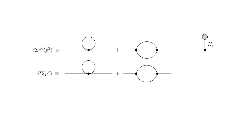 Figure 1
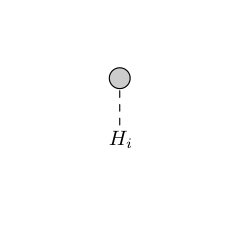 Figure 2
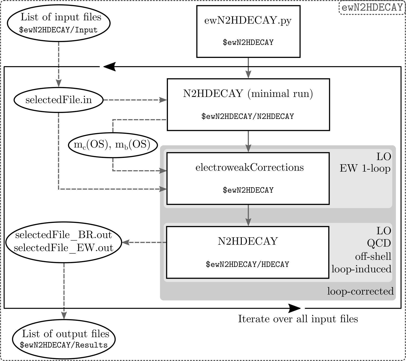 Figure 3
| -type | -type | leptons | |
| I | |||
| II | |||
| lepton-specific | |||
| flipped |
| N2HDM type | ||||||
| I | ||||||
| II | ||||||
| lepton-specific | ||||||
| flipped |
| Line | Input name | Allowed values and meaning |
| 6 | OMIT ELW2 | 0: electroweak corrections (N2HDM) are calculated 1: electroweak corrections (N2HDM) are neglected |
| 10 | N2HDM | 0: considered model is not the N2HDM 1: considered model is the N2HDM |
| 58 | TYPE | 1: N2HDM type I 2: N2HDM type II 3: N2HDM lepton-specific 4: N2HDM flipped |
| 76 | RENSCHEM | 0: all renormalization schemes are calculated 1-10: only the chosen scheme (cf. Tab. 6) is calculated |
| 77 | REFSCHEM | 1-10: the input values of , , and (cf. Tab. 5) are given in the chosen reference scheme and at the scale given by INSCALE in case of parameters; the values of , , and in all other schemes and at the scale at which the decays are calculated, are evaluated using Eqs. (2.105) and (2.106) |
| Line | Input name | Name in Sec. 2 | Allowed values and meaning |
| 19 | ALS(MZ) | strong coupling constant (at ) | |
| 20 | MSBAR(2) | -quark mass at 2 GeV in GeV | |
| 21 | MCBAR(3) | -quark mass at 3 GeV in GeV | |
| 22 | MBBAR(MB) | -quark mass at in GeV | |
| 23 | MT | -quark pole mass in GeV | |
| 24 | MTAU | -lepton pole mass in GeV | |
| 25 | MMUON | -lepton pole mass in GeV | |
| 26 | 1/ALPHA | inverse fine-structure constant (Thomson limit) | |
| 27 | ALPHAMZ | fine-structure constant (at ) | |
| 30 | GAMW | partial decay width of the boson | |
| 31 | GAMZ | partial decay width of the boson | |
| 32 | MZ | boson on-shell mass in GeV | |
| 33 | MW | boson on-shell mass in GeV | |
| 34-42 | Vij | CKM matrix elements ( , ) | |
| 60 | TGBET2HDM | ratio of the VEVs in the 2HDM | |
| 61 | M_12^2 | squared soft--breaking scale in GeV2 | |
| 66 | MHA | CP-odd Higgs boson mass in GeV | |
| 67 | MH+- | charged Higgs boson mass in GeV | |
| 78 | INSCALE | renormalization scale for inputs in GeV | |
| 79 | OUTSCALE | renormalization scale for the evaluation of the | |
| partial decay widths in GeV or in terms of MIN | |||
| 80 | MH1 | mass of the CP-even Higgs boson in GeV | |
| 81 | MH2 | mass of the CP-even Higgs boson in GeV | |
| 82 | MH3 | mass of the CP-even Higgs boson in GeV | |
| 83 | alpha1 | CP-even Higgs mixing angle in radians | |
| 84 | alpha2 | CP-even Higgs mixing angle in radians | |
| 85 | alpha3 | CP-even Higgs mixing angle in radians |
| Input ID | Tadpole scheme | Gauge-par.-indep. | ||
| 1 | standard | KOSY | KOSY (odd) | ✗ |
| 2 | standard | KOSY | KOSY (charged) | ✗ |
| 3 | alternative (FJ) | KOSY | KOSY (odd) | ✗ |
| 4 | alternative (FJ) | KOSY | KOSY (charged) | ✗ |
| 5 | alternative (FJ) | -pinched | -pinched (odd) | ✓ |
| 6 | alternative (FJ) | -pinched | -pinched (charged) | ✓ |
| 7 | alternative (FJ) | OS-pinched | OS-pinched (odd) | ✓ |
| 8 | alternative (FJ) | OS-pinched | OS-pinched (charged) | ✓ |
| 9 | standard | ✗ | ||
| 10 | alternative (FJ) | ✓ |
Peer Reviews
No public reviews on file for this paper yet. If you reviewed it on a platform where reviews are public (OpenReview, ICLR, NeurIPS, ICML), you can paste yours below so the community can read it here.
Code & Models
Videos
No videos yet. Explain this paper in a talk, walkthrough, or lecture? Add one.
h KA-TP-05-2019
ewN2HDECAY - A program for the Calculation of Electroweak One-Loop Corrections to Higgs Decays in the Next-to-Minimal Two-Higgs-Doublet Model Including State-of-the-Art QCD Corrections
Marcel Krause111E-mail: [email protected], Margarete Mühlleitner222E-mail: [email protected]
1Institute for Theoretical Physics, Karlsruhe Institute of Technology,
*Wolfgang-Gaede-Str. 1, 76131 Karlsruhe, Germany.
Abstract
We present in this paper our new program package ewN2HDECAY for the calculation of the partial decay widths and branching ratios of the Higgs bosons of the Next-to-Minimal 2-Higgs Doublet Model (N2HDM). The N2HDM is based on a general CP-conserving 2HDM which is extended by a real scalar singlet field. The program computes the complete electroweak one-loop corrections to all non-loop-induced two-body on-shell Higgs boson decays in the N2HDM and combines them with the state-of-the-art QCD corrections that are already implemented in the existing program N2HDECAY. Most of the independent input parameters of the electroweak sector of the N2HDM are renormalized in an on-shell scheme. The soft--breaking squared mass scale and the vacuum expectation value of the singlet field, however, are renormalized with conditions, while for the four scalar mixing angles () and of the N2HDM, several different renormalization schemes are applied. By giving out the leading-order and the loop-corrected partial decay widths separately from the branching ratios, the program ewN2HDECAY not only allows for phenomenological analyses of the N2HDM at highest precision, it can also be used for a study of the impact of the electroweak corrections and the remaining theoretical uncertainty due to missing higher-order corrections based on a change of the renormalization scheme. The input parameters are then consistently calculated with a parameter conversion routine when switching from one renormalization scheme to the other. The latest version of the program ewN2HDECAY can be downloaded from the URL https://github.com/marcel-krause/ewN2HDECAY.
1 Introduction
The discovery of the Higgs boson by the LHC experiments ATLAS [1] and CMS [2] has been a tremendous success for particle physics. The Standard Model (SM)-like behaviour of the discovered Higgs boson [3], on the other hand, leaves many questions open. To solve these problems, extensions beyond the SM (BSM) are considered, which usually entail enlarged Higgs sectors. In view of the lack of any direct experimental sign of new physics (NP) so far, indirect searches for NP in the Higgs sector become increasingly important. Due to the very SM-like nature of the discovered Higgs boson and because of the similarity of signatures predicted by different models, such searches require sophisticated experimental techniques on the one side and high-precision predictions by theory on the other side. This renders the inclusion of higher-order corrections in the Higgs boson observables indispensable. We contribute to this effort with the program code that we present and publish here. In an earlier work [4], we have published the code 2HDECAY for the computation of the electroweak (EW) corrections to the on-shell non-loop induced Higgs decays of the 2-Higgs-Doublet Model (2HDM). Here, we present the code ewN2HDECAY. It computes the EW corrections to the on-shell non-loop induced Higgs decays of the Next-to-2HDM (N2HDM). The N2HDM is based on the CP-conserving 2HDM extended by a real scalar singlet field. After electroweak symmetry breaking (EWSB) the Higgs sector consists of three neutral CP-even, one neutral CP-odd and two charged Higgs bosons. Due to its enlarged parameter space and its fewer symmetries compared with supersymmetric models it provides an interesting phenomenology with a variety of non-SM-like signatures that are still compatible with current experimental constraints [5, 6, 7]. Depending on which of its global symmetries are broken, its phenomenology can change considerably [8]. Thus it can feature a dark sector and extra sources of CP violation that only exist in the dark sector [9]. In [10], we computed the EW corrections to the Higgs boson decays in the N2HDM and provided a gauge-independent renormalization of the N2HDM. For this, we had to extend our formalism developed for the 2HDM in [11, 12, 13]333For later works discussing the renormalization of the 2HDM, see [14, 15, 16, 17, 18]. An improved on-shell scheme that is essentially equivalent to the mixing angle renormalization scheme presented by our group in [11, 12, 13] is used in [19, 20, 21]. to the N2HDM.
We have implemented 10 different renormalization schemes in ewN2HDECAY for the calculation of the EW corrections to the N2HDM Higgs decays into all possible on-shell two-particle final states of the model that are not loop-induced. The program is linked with the Fortran code N2HDECAY [5]. Based on an extension of the Fortran code HDECAY [22, 23], N2HDECAY incorporates the state-of-the-art higher-order QCD corrections to the decays including also loop-induced and off-shell decays. We consistently combine these corrections with our newly provided N2HDM EW corrections, so that ewN2HDECAY provides the N2HDM Higgs boson decay widths at the presently highest possible level of precision. Moreover, we separately give out the leading order (LO) and next-to-leading order (NLO) EW-corrected decay widths so that studies can be performed on the importance of the relative EW corrections. The comparison of the results for different renormalization schemes additionally allows to estimate the remaining theoretical uncertainty due to missing higher-order corrections. For the consistent comparison we include in ewN2HDECAY a routine that automatically converts the input parameters from one renormalization scheme to another for all 10 implemented renormalization schemes.
The development of ewN2HDECAY tightly followed the development of 2HDECAY, from which large parts of code were adapted for the calculation of the Higgs boson decays in the N2HDM. Due to the similarities of the two codes, similarities between the structure of this paper and the manual of 2HDECAY, cf. Ref. [4], are intentional. We still keep the description of ewN2HDECAY here as short as possible while at the same time taking care to remain self-contained. For additional details, we refer to [4] where appropriate.
The program ewN2HDECAY was developed and tested under Windows 10, openSUSE Leap 15.0 and macOS Sierra 10.12. In order to compile and run the program, an up-to-date version of Python 2 or Python 3 (tested with versions 2.7.14 and 3.5.0), the FORTRAN compiler gfortran and the GNU C compilers gcc (tested for compatibility with versions 6.4.0 and 7.3.1) and g++ are required. The latest version of the package can be downloaded from
https://github.com/marcel-krause/ewN2HDECAY .
The paper is organized as follows. In the subsequent Sec. 2, we briefly introduce the N2HDM and its particle content, focusing solely on the differences with respect to the 2HDM due to its extended scalar sector. Moreover, we introduce the relevant input parameters and set our notation. We briefly present the counterterms of the extended scalar sector that are needed for the computation of the EW corrections as well as changes in the counterterms with respect to the 2HDM. A full list of the decays implemented in ewN2HDECAY is presented, the link to N2HDECAY is described and the parameter conversion is discussed. In Sec. 3, we introduce the program ewN2HDECAY, describe its structure in detail and provide an installation and usage guide. Moreover, we briefly describe the required format of the input and output file and the meaning of the input parameters. We complete the paper with a short summary of our work in Sec. 4. As a useful reference for the user, we print the exemplary input and output files which are included in the ewN2HDECAY repository, in Appendices A and B, respectively.
2 One-Loop Electroweak and QCD Corrections in the N2HDM
After a brief introduction of the N2HDM where we set up our notation and list the input parameters used for the calculation we present the renormalization of the EW sector of the N2HDM that we apply in the computation of the EW one-loop corrections to the partial decay widths of the neutral N2HDM Higgs bosons. We shortly describe the computation of these partial decay widths and explain how the EW-corrected partial decay widths are combined with the state-of-the-art QCD corrections already implemented in the code N2HDECAY.
2.1 Introduction of the N2HDM
We consider a general CP-conserving N2HDM which, in comparison to the 2HDM, is extended by adding a real singlet field with hypercharge . Together with the two complex doublets and with hypercharges , it builds the scalar sector of the model. Through EWSB, the two doublet and the singlet fields develop non-negative real vacuum expectation values (VEVs) , and , which in general are non-vanishing. The doublet and singlet fields can be expanded around these VEVs as
[TABLE]
where and are three CP-even fields, are two CP-odd fields and are two electromagnetically charged fields (). The two VEVs of the doublets are connected to the SM VEV via the relation
[TABLE]
The ratio of the two VEVs defines the characteristic parameter given by
[TABLE]
The EW part of the Lagrangian relevant for our computation of the EW one-loop corrections is given by
[TABLE]
The Yang-Mills Lagrangian and the fermion Lagrangian are analogous to the SM. Their explicit forms are presented e.g. in [24, 25]. We do not present the explicit forms of the gauge-fixing Lagrangian and Fadeev-Popov Lagrangian as they are not needed in the following. We remark, however, that we follow the same approach as in [26] for the 2HDM and apply the gauge-fixing procedure only after the renormalization of the N2HDM is performed so that contains only renormalized fields and no additional counterterms for the gauge-fixing terms need to be introduced. The interaction of the Higgs bosons with the fermions is derived from the Yukawa Lagrangian , with the corresponding Yukawa couplings presented e.g. in [5].
The scalar Lagrangian with the kinetic terms of the Higgs doublets and the scalar N2HDM potential reads
[TABLE]
where denotes the covariant derivative
[TABLE]
with the gauge couplings and and the corresponding gauge boson fields and of the and , respectively. The generators of the gauge group are given by the Pauli matrices . The scalar potential of the CP-conserving N2HDM is given by
[TABLE]
where denotes the scalar potential of the CP-conserving 2HDM, as given by [27]
[TABLE]
It is obtained by imposing two symmetries on the scalar potential, under one of which, ,
[TABLE]
It is the trivial generalisation of the usual 2HDM symmetry (guaranteeing the absence of tree-level flavour-changing neutral currents (FCNCs) when extended to the Yukawa sector) and explicitly broken by the term proportional to . The second symmetry, , under which
[TABLE]
is not explicitly broken. The N2HDM potential contains twelve real-valued parameters, four mass parameters , , and and eight dimensionless coupling constants (). For later convenience, we define
[TABLE]
Inserting the expansion of the scalar doublet and singlet fields, Eq. (2.1), into the scalar potential of the N2HDM yields
[TABLE]
where denotes the mass matrix in the CP-even scalar sector and , and the three tadpole terms. We demand that the VEVs represent the minimum of the potential by applying the minimum condition
[TABLE]
leading at tree level to the vanishing of the three tadpole terms,
[TABLE]
which in terms of the Higgs potential parameters read
[TABLE]
These conditions can be used to replace , and in favor of the three tadpole terms. The mass matrix of the CP-even scalar fields is given by
[TABLE]
By introducing three mixing angles () defined in the range
[TABLE]
the mass matrix can be diagonalised by means of the orthogonal matrix parametrised as444Throughout this paper, we use the short-hand notation , and .
[TABLE]
which transforms the CP-even interaction fields into the mass eigenstates ()
[TABLE]
This transformation yields the diagonalised mass matrix
[TABLE]
where we demand the three CP-even Higgs bosons to be ordered by ascending mass,
[TABLE]
The CP-odd and charged mass matrices, not shown explicitly in Eq. (2.12) are equivalent to the ones in the 2HDM and are diagonalised by the two mixing angles and , respectively, which, at tree level, coincide with the angle defined in Eq. (2.3). The rotation of the corresponding fields to the mass basis yields the CP-odd and charged Higgs bosons and with masses and , respectively, as well as the massless CP-odd and charged Goldstone bosons and . The quartic couplings () of the N2HDM potential can be written in terms of the parameters of the mass basis as [5]
[TABLE]
The gauge sector of the N2HDM does not change with respect to the SM. After EWSB we have for the masses of the physical gauge bosons, the and bosons and the photon,
[TABLE]
The electromagnetic coupling in terms of the fine-structure constant , which we use as independent input, reads
[TABLE]
Alternatively, the tree-level relation to the Fermi constant,
[TABLE]
can be used to replace one of the parameters of the EW sector in favour of .
The aforementioned softly broken symmetry, Eq. (2.9), for the two doublet fields and , extended to the Yukawa sector to avoid FCNCs at tree level, leads to four types of doublet couplings to the fermion fields as in the 2HDM. They are summarised in Tab. 1. The Yukawa couplings can be parametrised in terms of the Yukawa coupling parameters () summarised in Tab. 2, where refers the the scalar Higgs bosons and 4 to the pseudoscalar .
Apart from the parameters introduced so far, N2HDECAY requires additional input parameters, namely the electromagnetic fine-structure constant in the Thomson limit for the computation of the loop-induced decays into and , the strong coupling constant for the calculation of the loop-induced decays into gluons as well as for the state-of-the-art QCD corrections, and additionally the total decay widths and of the and bosons, respectively, for the calculation of the off-shell decays into pairs of these gauge bosons. Moreover, the CKM matrix elements are required as input for the computation of the decays involving charged quark currents, as well as the quark masses , where – all other fermions are approximated to be massless in the computation of the partial decay widths. The fermion and gauge boson masses are defined according to the recommendations of the LHC Higgs cross section working group [28]. Note that in N2HDECAY the decay widths are computed in terms of the Fermi constant with the exception of the decays involving external on-shell photons which are given in terms of in the Thomson limit. As input for our renormalization conditions of the EW corrections, we require as input parameters, however, the on-shell masses and and the electromagnetic coupling at the boson mass scale, . We will come back to this in Sec. 2.4. The full set of independent input parameters in the mass basis therefore is given by ()
[TABLE]
For completeness, we want to mention that the three tadpole parameters , and are formally independent input values, as well. However, as we explain in the upcoming Sec. 2.2.1, these parameters are either zero after renormalization or they are not present in the theory in the first place within an alternative treatment of the minimum conditions of the potential. In both cases, the parameters are effectively required to vanish and hence, we do not include them in the set of independent input parameters.
2.2 Renormalization
The ultraviolet (UV) divergences appearing in the one-loop corrections to the decay widths calculated in this work require the renormalization of the relevant parameters entering the decay widths at tree level. Apart from an extended CP-even scalar sector, the N2HDM is equivalent to the 2HDM at tree level so that the one-loop renormalization of the N2HDM can be performed analogously to the 2HDM. In the following, we only present the renormalization of the extended CP-even scalar sector of the N2HDM, i.e. we describe only the changes of the renormalization with respect to the 2HDM. For a thorough discussion of the renormalization of the N2HDM in general, we refer to [10] and for the definition of the 2HDM-like counterterms (CTs) as they are incorporated into ewN2HDECAY, we refer to [11, 12, 13, 4].555The renormalization of the 2HDM is also discussed in detail in [14, 15] and in [17], the renormalization of mixing angles in general and the application to the 2HDM in particular is discussed. In [18, 29], the gauge-independent renormalization of multi-Higgs models is described.
Most of the N2HDM input parameters given in Eq. (2.37) are renormalized with on-shell (OS) conditions. For the physical masses, this leads to their counterterms being defined as the real parts of the poles of the propagators of the corresponding fields. All physical fields are equivalently renormalized in an OS approach, i.e. we demand that on the mass shell, no mixing of fields with the same quantum numbers takes place. The residues of the propagators associated to the corresponding fields are normalized to unity so that the fields are properly normalized as well. The soft--breaking parameter and the singlet vacuum expectation value are renormalized via conditions. For the scalar mixing angles () and , several different renormalization schemes are implemented.
2.2.1 Renormalization of the Tadpoles
As discussed e.g. in [11, 12], the proper renormalization of the ground state of the Higgs potential is crucial for defining gauge-independent counterterms for the scalar mixing angles. We have implemented two different procedures in ewN2HDECAY that we briefly introduce666For further information, see [11, 12, 4, 10] where they have been discussed in detail. before presenting the related renormalization conditions.
At NLO the tadpole terms are replaced by
[TABLE]
where the at the right-hand side denote the renormalized tadpole terms and the corresponding CTs. In the standard tadpole scheme, used e.g. in [25] for the SM and in [30, 31] for the 2HDM, the tadpole terms, which define the ground state of the Higgs potential, are renormalized such that the potential remains at the correct minimum at higher orders. This implies the renormalization conditions at one-loop level and eventually leads to the identification of the tadpole CTs with the corresponding genuine one-loop tadpole diagrams . Denoting the counterterms and one-loop tadpole diagrams in the mass basis by and , respectively, we have
[TABLE]
The tadpole CTs in the mass basis are related to those in the gauge basis, , through the rotation with the mixing matrix defined in Eq. (2.21),
[TABLE]
The tadpole terms appear in the diagonal entries of all scalar mass matrices, cf. e.g. Eq. (2.18). After their diagonalisation, cf. Eq. (2.22), this leads to twelve different tadpole CTs at NLO, given by
(2.43)
(2.44)
(2.45)
(2.46)
(2.47)
(2.48)
(2.49)
The renormalization conditions of Eq. (2.39) imply that no tadpole diagrams have to be taken into account in the calculation of partial decay widths at one-loop level apart from the CTs of the scalar mass matrices, in which the tadpole terms explicitly appear and as a consequence, the tadpole CTs in the mass basis from Eqs. (2.43)-(2.49) appear in the off-diagonal scalar wave function renormalization counterterms (WFRCs) and mass CTs, cf. Sec. 2.2.3.
With the VEVs in the standard tadpole scheme being defined as the minimum of the loop-corrected gauge-dependent potential, they are consequently gauge-dependent as well, as are all other CTs defined through this minimum like e.g. the mass CTs of the Higgs and gauge bosons. While this is no problem as long as all gauge dependences in the calculation of the loop-corrected decay widths cancel, an improper renormalization condition for the mixing angle CTs in the N2HDM (and also the 2HDM) can lead to residual gauge dependences that spoil the overall gauge independence of the partial decay widths as discussed in more detail in Sec. 2.2.4.
In the framework of the alternative (FJ) tadpole scheme, based on the work by J. Fleischer and F. Jegerlehner in the SM, cf. Ref. [32], and applied to the 2HDM for the first time in Refs. [11, 12], the so-called proper VEVs are defined as the true ground state of the Higgs potential, i.e. as the renormalized all-order VEVs of the Higgs fields. In this alternative framework, the VEVs are defined through the gauge-independent tree-level potential instead of the loop-corrected gauge-dependent one so that they become manifestly gauge-independent quantities and thereby also the mass (matrix) CTs become manifestly gauge-independent. Being the fundamental quantities in the alternative tadpole schemes, the VEVs - instead of the tadpole terms - are shifted as
[TABLE]
where the CTs () are fixed by demanding that the renormalized VEVs represent the proper tree-level minima of the Higgs potential to all orders. This renormalization condition connects the CTs of the VEVs with explicit tadpole diagrams as follows:
[TABLE]
The renormalization of the minimum of the potential in the alternative tadpole scheme implies a shift of the VEVs by additional tadpole contributions. These have to be considered everywhere in the N2HDM where the three VEVs , and appear. Consequently, all self-energies used for the definition of the CTs acquire additional one-particle-reducible tadpole contributions compared to the usual one-particle-irreducible self-energies , cf. Fig. 1. In the calculation of the one-loop vertex corrections the tadpole diagrams have to be taken into account as well, so that the alternative tadpole scheme is characterized by the following conditions:
(2.52)
(2.53)
Tadpole diagrams have to be considered in the vertex corrections.
2.2.2 Renormalization of the Gauge Sector
The gauge sector of the N2HDM does not differ from that of the 2HDM. We implement the same renormalization conditions of the gauge sector as presented in [4] for the 2HDM. Formally, all CTs are the same as stated there, they only differ in the particle content of the two-point functions used for the definition of the CTs of the N2HDM due to the extended scalar sector. We therefore do not state them explicitly here and refer to [4] for details.
2.2.3 Renormalization of the Scalar Sector
The fields and masses of the CP-even scalar particles are shifted at one-loop level as
[TABLE]
All scalar fields are renormalized through OS conditions implying the following CT and WFRC definitions,
\displaystyle=\frac{2}{m_{H_{i}}^{2}-m_{H_{j}}^{2}}\textrm{Re}\Big{[}\Sigma_{H_{i}H_{j}}(m_{H_{j}}^{2})-\delta T_{H_{i}H_{j}}\Big{]}~{}~{}~{}(i\neq j)~{},
(2.56)
\displaystyle=\textrm{Re}\Big{[}\Sigma_{H_{i}H_{i}}(m_{H_{i}}^{2})-\delta T_{H_{i}H_{i}}\Big{]}~{},
(2.57)
\displaystyle=\frac{2}{m_{H_{i}}^{2}-m_{H_{j}}^{2}}\textrm{Re}\Big{[}\Sigma^{\textrm{tad}}_{H_{i}H_{j}}(m_{H_{j}}^{2})\Big{]}~{}~{}~{}(i\neq j)~{},
(2.58)
\displaystyle=\textrm{Re}\Big{[}\Sigma^{\textrm{tad}}_{H_{i}H_{i}}(m_{H_{i}}^{2})\Big{]}~{},
(2.59)
(2.60)
where the tadpole CTs in the standard scheme are given in Eq. (2.43). The renormalization of the other scalar particles of the N2HDM, namely of the CP-odd and charged Higgs bosons and and the Goldstone bosons and , is equivalent to their renormalization within the 2HDM and the CTs are implemented as presented in [4].
2.2.4 Renormalization of the Scalar Mixing Angles
The bare mixing angles () and are promoted to one-loop order by introducing their CTs () and according to
[TABLE]
where the mixing angles on the right-hand side are the renormalized ones. In the following, we briefly describe the different renormalization schemes for the scalar mixing angles that are implemented in ewN2HDECAY. For a detailed derivation and description of these schemes, we refer to [10].
** scheme.** It has been shown in Refs. [33, 11] for the 2HDM that the one-loop corrected partial decay widths can become very large when the mixing angles are renormalized in the scheme and while this can also be expected in the N2HDM, we nevertheless implemented the scheme for the scalar mixing angles as a reference scheme. By imposing conditions, only UV-divergent parts are assigned to the four mixing angle CTs, but no finite parts () and . After having checked explicitly for UV finiteness of all partial decay widths, the mixing angle CTs in the scheme are implemented in ewN2HDECAY by effectively setting them to zero:
(2.63)
(2.64)
As a consequence of the renormalization, the CTs and become a function of the renormalization scale . This scale at which the mixing angles and their CTs are given has to be specified explicitly by the user in the input file of ewN2HDECAY. The one-loop corrected partial decay widths that contain these CTs also depend on the scale . Moreover, the one-loop partial decay widths depend on another scale at which the loop integrals are evaluated. The latter scale should be chosen appropriately to avoid the appearance of large logarithms in the partial decay widths. In case that the two scales and are chosen to be different, the parameter conversion automatically converts the scalar mixing angles from the scale to , as further described in Sec. 2.5. For this conversion, the UV-divergent terms of the mixing angle CTs are required, which were extracted and implemented analytically by isolating the UV-divergent pieces of the mixing angle CTs as defined in an arbitrary other renormalization scheme.
Adapted KOSY scheme. For the renormalization of the scalar mixing angles in the 2HDM, the KOSY scheme (denoted by the authors’ initials) was proposed in Ref. [30]. It can be directly adapted to the renormalization of the four mixing angles in the N2HDM as detailed in Ref. [10]. The adapted KOSY scheme connects the definition of the scalar mixing angle CTs to the off-diagonal scalar WFRCs by temporarily switching from the mass basis to the interaction basis before promoting the mixing angles to one-loop order. While the KOSY scheme not only leads to gauge-dependent mixing angle CTs but also to residual gauge dependences in the partial decay widths, we implement this scheme for comparative studies with the other schemes only. Due to the residual gauge dependences, we do not recommend it for actual use in phenomenological analyses, however. The CTs in the adapted KOSY scheme are given by
(2.65)
(2.66)
(2.67)
(2.68)
(2.69)
(2.70)
(2.71)
(2.72)
(2.73)
(2.74)
Like in 2HDECAY, cf. [4], we implemented two versions of the KOSY scheme in ewN2HDECAY that differ with respect to the WFRCs through which the CT is defined, namely and which define the CT through the WFRCs of the CP-odd and the charged scalar sector, respectively.
-pinched scheme. The (adapted) KOSY scheme can be modified such that a gauge-parameter-independent definition of the mixing angle CTs is achieved. This approach was suggested in Refs. [11, 12] for the 2HDM and in Ref. [10] for the N2HDM. The derivation of the mixing angle CTs is analogous to the (adapted) KOSY scheme, but instead of defining them over the usual off-diagonal WFRCs, the self-energies are replaced by the pinched self-energies which are derived by means of the pinch technique (PT), cf. Refs. [34, 35, 36, 37, 38, 39, 40, 41]. For consistency and the cancellation of all gauge dependences, the alternative tadpole scheme is necessarily required for this renormalization scheme of the mixing angle CTs. The pinched scalar self-energies are equivalent to the self-energies in the alternative tadpole scheme up to additional self-energy-like contributions . In the -pinched scheme, adapted from Ref. [42] in the Minimal Supersymmetric Extension of the SM (MSSM), the pinched self-energies are evaluated at the scale
[TABLE]
At this scale, the additional self-energy-like contributions vanish. The scalar mixing angle CTs are then given as follows:
(2.76)
(2.77)
(2.78)
(2.79)
(2.80)
As for the adapted KOSY scheme, we implemented two different variations of the -pinched scheme that differ in the definition of the CT of . The index ’’ means that the self-energies are evaluated in the Feynman gauge.
OS-pinched scheme. In the OS-pinched scheme, the pinched scalar self-energies are evaluated at the OS-inspired mass scale of the corresponding scalar particle. In this case, the additional UV-divergent777While the additional self-energy-like contributions are all separately UV-divergent, they appear only in UV-finite combinations in the definition of the mixing angle CTs (), cf. Ref. [4]. self-energy-like contributions do not vanish. They were derived for the N2HDM in Ref. [4] and read
[TABLE]
where and () is a shorthand notation for the following combinations of coupling constants between the Higgs and gauge sectors as defined in Tab. 3:
[TABLE]
The mixing angle CTs in the OS-pinched scheme are given by:
(2.87)
(2.88)
(2.89)
(2.90)
(2.91)
2.2.5 Renormalization of the Fermion Sector
The renormalization of the fermion sector in the N2HDM is performed as in the 2HDM. All CTs of the fermion masses, the CKM mixing matrix elements and the fermion WFRCs are implemented with definitions analogous to those presented in [4]. The only difference with respect to the 2HDM are the different Yukawa couplings due to the extended scalar sector of the N2HDM. The CTs of the Yukawa coupling parameters defined in Tab. 2 are given by the following relations for which hold independently of the chosen N2HDM type:
[TABLE]
2.2.6 Renormalization of the Soft--Breaking Parameter
The soft--breaking Parameter is promoted to NLO by introducing a CT according to
[TABLE]
One possibility to fix the CT for is to define it via a Higgs-to-Higgs decay, since the Higgs self-couplings contain the parameter at tree level. However, such a process-dependent definition of has the drawback that the CT is defined not only via the genuine vertex corrections of the Higgs-to-Higgs decay, but additionally as a function of several other CTs of the N2HDM due to the intricate structure of the Higgs self-couplings. As a result, such a CT can introduce very large finite contributions which leads to NLO corrections that can become very large as well. This has already been observed in Ref. [13] in the context of the 2HDM. We therefore do not implement a process-dependent scheme for in ewN2HDECAY but instead fix the CT through an condition, i.e. only contains UV-divergent and some global finite parts parts proportional to
[TABLE]
where denotes the Euler-Mascheroni constant, denotes the mass-dimensional ’t Hooft scale which cancels in the calculation of decay amplitudes and the regulator is introduced in the framework of dimensional regularization, cf. Refs. [43, 44, 45, 46, 47]. In ewN2HDECAY, we extracted the UV divergence of by calculating the one-loop amplitude of the decay , including the genuine vertex corrections of the process as well as all CTs apart from , and by considering the residual UV divergence which is then assigned to . This yields the following analytic expression of the CT,
\displaystyle=\frac{\alpha_{\text{em}}m_{12}^{2}}{16\pi m_{W}^{2}\left(1-\frac{m_{W}^{2}}{m_{Z}^{2}}\right)}\Big{[}\frac{8m_{12}^{2}}{s_{2\beta}}-2m_{H^{\pm}}^{2}-m_{A}^{2}+\sum_{i=1}^{3}R_{i1}R_{i2}m_{H_{i}}^{2}-3(2m_{W}^{2}+m_{Z}^{2})
(2.98)
\displaystyle\hskip 14.22636pt+\sum_{u}6m_{u}^{2}Y^{u}_{4}\left(Y^{u}_{4}-\frac{1}{t_{2\beta}}\right)+\sum_{d}6m_{d}^{2}Y^{d}_{4}\left(Y^{d}_{4}-\frac{1}{t_{2\beta}}\right)+\sum_{l}2m_{l}^{2}Y^{l}_{4}\left(Y^{l}_{4}-\frac{1}{t_{2\beta}}\right)\Big{]}\Delta
where the sums are performed over all up- and down-type quarks as well as over all charged leptons, respectively. Since is a genuine parameter of the N2HDM Higgs potential before EWSB, it is gauge-independent and the CT is invariant under a change of the tadpole renormalization so that is the same in both tadpole schemes. Due to the renormalization of , the CT explicitly depends on the renormalization scale whose value has to be specified by the user888In ewN2HDECAY, all parameters are given at the same global scale .. In case that the renormalization scale at which the one-loop partial decay widths are evaluated differs from the input renormalization scale , the parameter conversion routine, cf. Sec. 2.5, evolves the parameter from to , analogous to the renormalized scalar mixing angles.
2.2.7 Renormalization of the singlet VEV
While the singlet VEV is already accounted for by the proper renormalization of the minimum of the Higgs potential, cf. Sec. 2.2.1, it still receives an additional CT after the minimum conditions are imposed on the one-loop potential. This is in analogy to the doublet VEVs. In the framework of e.g. the alternative tadpole scheme, the doublet VEVs and acquire shifts according to Eq. (2.50). These shifts ensure that the VEVs are equivalent to the gauge-independent tree-level VEVs of the potential, so that
[TABLE]
holds. After the minimum conditions are applied through the VEV shifts, the tree-level parameters and still need to be renormalized, so that effectively acquires an additional CT in form of a combination of CTs for and ,
[TABLE]
Analogously, the singlet VEV is shifted according to Eq. (2.50), ensuring that is equivalent to the tree-level singlet VEV in the alternative tadpole scheme, and after the minimum conditions of the potential are applied at one-loop order, acquires an additional CT through
[TABLE]
For more details about the appearance of these additional CTs, we refer to Ref. [10]. Transferring the general analysis on the renormalization of spontaneously broken gauge symmetries presented in Ref. [48] in the framework of the standard tadpole scheme to the N2HDM yields the conclusion that cannot contain UV divergences since the corresponding singlet field obeys a rigid invariance. Therefore, contains at most finite parts in the standard tadpole scheme which can be fixed e.g. in a process-dependent renormalization scheme. In ewN2HDECAY, we implemented conditions for the singlet VEV CT in order to avoid potentially large finite contributions that would be introduced in the CT when fixing it through a Higgs-to-Higgs decay. The CT is implemented by setting its finite part to zero:
(2.102)
As for renormalized scalar mixing angles and , the value of is converted from the input renormalization scale to the scale at which the decays are evaluated in case that both scales differ. For this conversion the UV-divergent parts of are needed. In the standard tadpole scheme, these UV-divergent parts are identically zero due to the rigid invariance, and as a consequence, the parameter is not converted and remains the same if the two scales are different999This corresponds to the vanishing of the one-loop beta function of in the standard tadpole scheme.. In the alternative tadpole scheme, however, contains additional UV divergences which have been extracted by calculating the remaining UV-divergent parts of the off-shell process to one-loop order when all CTs apart from are fixed. Due to the lengthy analytic expression of the UV-divergent parts of , we do not state them explicitly here.
2.3 Electroweak Decay Processes at LO and NLO
For the EW corrections, we only consider OS decay processes, i.e. the decays of all Higgs bosons with four-momentum into two particles and with four-momenta and , respectively, for which
[TABLE]
Note that we do not include here loop-induced tree-level decays, so that the EW one-loop corrections are calculated for the following processes (),
- •
()
- •
()
- •
()
- •
(, )
- •
( and )
- •
()
- •
()
- •
()
Like in 2HDECAY, we do not consider decays containing first-generation fermions, i.e. the decays (, ) and () are neglected in ewN2HDECAY.
From a technical point of view, the calculation of the LO and NLO decay amplitudes in ewN2HDECAY is identical to their calculation in the 2HDM in 2HDECAY. In the following, we only briefly mention the tools used for the calculation. For a more detailed explanation of the calculation, we refer to Ref. [4]. The Feynman amplitudes for the LO and NLO decays as well as for the tadpole diagrams and self-energies required for the definition of the CTs were generated with FeynArts 3.9 [49]. The N2HDM model file necessary for the generation of the amplitudes was created with SARAH 4.14.0 [50, 51, 52, 53, 54]. The simplification of the Dirac algebra, the Passarino-Veltman reduction and the analytic evaluation of the decay amplitudes as well as the CTs was performed with the help of the tool FeynCalc 8.2.0 [55, 56]. The real corrections necessary for the cancellation of all infra-red (IR) divergences were implemented analytically by applying the general results given in Ref. [57] to the N2HDM. For the evaluation of the integrals involved in the real corrections, the analytic expressions of Ref. [25] were implemented. The numerical evaluation of the loop integrals is performed by linking LoopTools 2.14 [58].
2.4 Link to N2HDECAY
For our new tool ewN2HDECAY we combine the EW one-loop corrections to the N2HDM Higgs decays with the Fortran code N2HDECAY. This code is based on an extension of the Fortran code HDECAY version 6.511 [22, 23] to the N2HDM [5, 8], which includes the state-of-the-art QCD corrections in the partial decay widths.101010Details can be found in [22, 23]. Care has to be taken when combining the two codes in order to remain consistent at higher loop level. We commented on this in detail in [4] and summarise here only very briefly the main points.
In order to consistently combine (N2)HDECAY which uses as independent input parameters with the EW-corrected decays based on the set as independent input parameters, we choose a pragmatic solution where the N2HDECAY decay widths in terms of are rescaled with , with being calculated through the tree-level relation Eq. (2.36) as a function of .111111The proper conversion between the and scheme would require the inclusion of N2HDM higher-order corrections in the conversion formulae. We expect the differences with respect to our pragmatic approach to be small. In case the user does not choose to calculate the EW corrections no such rescaling is performed. Note also that N2HDECAY includes off-shell decays in certain final states. In ewN2HDECAY the EW and QCD corrections are combined such that N2HDECAY computes the off-shell decay widths, but the EW corrections are only added to OS decays. We furthermore assume that the QCD and EW corrections factorize. The relative QCD corrections are defined with respect to the LO width that is calculated by N2HDECAY and contains e.g. also running quark masses in order to improve the perturbative behaviour. The relative EW corrections , however, are obtained by normalizing to the LO width with OS particle masses. The QCD and EW corrected decay width into a specific final state, , is hence calculated as
[TABLE]
The formula includes the aforementioned rescaling factor .
For each input file generically called inputfilename.in in the following121212The input filename can be chosen arbitrarily by the user., the program ewN2HDECAY provides two separate output files which adopt the filename of the input file together with additional suffices as explained in the following. The file inputfilename_BR.out contains both the total widths and branching ratios as calculated by N2HDECAY without the EW corrections131313We remind the reader that they include loop-induced and off-shell decays as well as QCD corrections where applicable. They are furthermore rescaled by in case the flag for the EW corrections is turned on in the input file. and those including the EW corrections based on the formula Eq. (2.104). In the file inputfilename_EW.out the LO and EW-corrected NLO decay widths are given out. Note that the LO widths do not contain any running quark masses here in decays into quark pair final states. Furthermore, the widths are calculated in the scheme. The widths given out here are not useful for phenomenological analyses as they do not include any QCD corrections nor loop-induced or off-shell decays. They can be used, however, for the study on the importance of the EW corrections and an estimate of the remaining theoretical uncertainty due to missing higher-order corrections by changing the renormalization schemes.
We finally remark that for certain parameter choices the EW-corrected decay widths can become negative. This can be due to a small LO width, due to an artificial enhancement of the EW corrections because of a badly chosen renormalization scheme or due to parametrically enhanced EW corrections because of large involved couplings. In this case, the NLO corrections cannot be trusted of course and should be discarded. For further details and discussions, we refer to [12, 13, 10, 4].
2.5 Parameter Conversion
The one-loop corrected partial decay widths explicitly depend on the renormalization scale at which the integrals of the higher-order corrections are evaluated. In ewN2HDECAY, this scale can be chosen by the user to be either at a fixed global value or to be equal to the mass of the decaying particle. Additionally, all renormalized parameters introduce a dependence on the input renormalization scale at which these parameters are defined. This scale has to be given by the user in the input file. In case the two scales and differ, the parameters need to be converted from the input scale to the output scale , which is done by means of the formula
[TABLE]
where and denote all parameters (, and () and , if the latter are defined in an scheme) and their respective CTs. The superscript ’div’ indicates that only the UV-divergent part of the CT is taken into account.
Apart from the conversion of the parameters from one scale to another, an additional parameter conversion of the scalar mixing angles has to be performed if the renormalization scheme at which their input is given is different from the renormalization scheme with which the one-loop partial decay widths are evaluated. Since the 10 different renormalization schemes implemented in ewN2HDECAY differ only in their definition of the mixing angle CTs, the scalar mixing angles are the only parameters affected by the parameter conversion. The values of the mixing angles given in the reference scheme, i.e. , and their values in another different renormalization scheme are connected to each other via the bare values of the mixing angles, which are independent of the renormalization scheme. Together with the corresponding CTs and in the two different schemes, the conversion of the values is given by
[TABLE]
This linearized relation holds approximately up to higher-order terms, since the CT on the right-hand side is evaluated with the parameters given in the reference scheme instead of the other renormalization scheme in which is defined. We want to emphasize that Eq. (2.106) also contains a dependence on the scales and which is of importance if the scalar mixing angels are defined in an scheme.
3 Program Description
In this section, we describe the system requirements for ewN2HDECAY and provide a guide for installing and using the program. Moreover, we describe the format of the input and output files in detail.
3.1 System Requirements
The Python/FORTRAN program code ewN2HDECAY was developed under Windows 10 and openSUSE Leap 15.0. The following operating systems are supported:
- •
Windows 7 and Windows 10 (tested with Cygwin 2.10.0)
- •
Linux (tested with openSUSE Leap 15.0)
- •
macOS (tested with macOS Sierra 10.12)
The compilation of ewN2HDECAY under Windows requires an installed up-to-date version of Cygwin (together with the packages cURL, find, gcc, g++ and gfortran). For the compilation of ewN2HDECAY the GNU C compilers gcc (tested with versions 6.4.0 and 7.3.1), g++ and the FORTRAN compiler gfortran are needed. Additionally, an up-to-date version of either Python 2 or Python 3 are required (tested with versions 2.7.14 and 3.5.0).
3.2 License
ewN2HDECAY is released under the GNU General Public License (GPL) (GNU GPL-3.0-or-later). ewN2HDECAY is free software, which means that anyone can redistribute it and/or modify it under the terms of the GNU GPL as published by the Free Software Foundation, either version 3 of the License, or any later version. ewN2HDECAY is distributed without any warranty. A copy of the GNU GPL is included in the LICENSE.md file in the root directory of ewN2HDECAY.
3.3 Download
The latest version of the program package ewN2HDECAY can always be obtained from the url https://github.com/marcel-krause/ewN2HDECAY. The user can either clone the repository or download the whole program as a zip archive. The directory for the installation that is chosen by the user will in the following be referred to as $ewN2HDECAY. The main folder of ewN2HDECAY contains several subfolders:
BuildingBlocks
Here the analytic EW one-loop corrections for all considered decays can be found, as well as the CTs and real corrections needed for the UV and IR finiteness of the decay widths.
Documentation
Contains this documentation.
N2HDECAY
This subfolder contains a modified version of N2HDECAY [22, 23, 5]. It computes the LO and (where applicable) QCD corrected decay widths as well as off-shell decay widths and the loop-induced decay widths into gluon and photon pair final states and into . N2HDECAY also computes the branching ratios.
Input
Here, at least one or more input files which shall be used for the computation are stored. In Sec. 3.5 the format of the input file is explained. In the Github repository, we provide the exemplary input file depicted in App. A in the folder Input.
Results
In this subfolder the results of a successful run of ewN2HDECAY are stored as output files. They have the same name as the corresponding input files in the Input folder, but with the file extension .in replaced by .out and a suffix “_BR” and “_EW” for the branching ratios and EW partial decay widths, respectively. In the Github repository, we provide the exemplary output files which are printed in App. B in the folder Results.
The main folder $ewN2HDECAY also contains several files:
ewN2HDECAY.py
This is the main program file of ewN2HDECAY. It serves as a wrapper file that calls N2HDECAY for the conversion of the charm and bottom quark masses from the input values to the corresponding OS values and for the computation of the LO widths, QCD corrections, off-shell and loop-induced decays and the branching ratios. It also calls electroweakCorrections for the calculation of the EW one-loop corrections.
Changelog.md
Documents all changes made in the ewN2HDECAY since version 1.0.0.
CommonFunctions.py
A library of functions frequently used in the different files of the program ewN2HDECAY.
Config.py
Main configuration file. In case LoopTools is not installed automatically by the installer of ewN2HDECAY, the paths to the LoopTools executables and libraries have to be set manually in this file.
constants.F90
Library for all constants used in ewN2HDECAY.
counterterms.F90
Here all fundamental CTs necessary for the EW one-loop renormalization of the Higgs boson decays are defined. These CTs require the analytic results saved in the BuildingBlocks subfolder.
electroweakCorrections.F90
Main file for the calculation of the EW one-loop corrections to the Higgs boson decays. The EW one-loop corrections to the decay widths are combined with the necessary CTs and real corrections for the EW contributions to the tree-level decay widths that are then combined with the QCD corrections in N2HDECAY.
getParameters.F90
Routine to read in the input values given by the user in the input files that are needed by ewN2HDECAY.
LICENSE.md
Contains the full GNU General Public License (GNU GPL-3.0-or-later) agreement.
README.md
Provides an overview over basic information about the program as well as a quick-start guide.
setup.py
Main setup and installation file of ewN2HDECAY. For a guided installation, this file should be called after downloading the program.
3.4 Installation
For the installation of ewN2HDECAY, we recommend to use the automatic installation script setup.py which is part of the ewN2HDECAY repository and which guides the user through the installation. If ewN2HDECAY is installed under Windows, the user should first install Cygwin and check whether the path to the Cygwin executable in line 36 of the configuration file ewN2HDECAY and executes the following command:
python setup.py
First, the script asks whether the LoopTools version specified in line 37 of 2HDECAY/Config.py should be downloaded and installed. By typing y, the specified version of LoopTools is automatically installed in a subdirectory of ewN2HDECAY. For a more detailed description of the installation of the program, we refer to [[58](#bib.bib58)]. The installation of LoopTools is optional if the user already has a current working version of the program on the system. The installation of LoopTools can then be skipped. However, in this case the lines 33-35 of the configuration file 2HDECAY/Config.py need to be modified in order to specify the path to the LoopTools executables and libraries. Moreover, line 32 has to be set to
useRelativeLoopToolsPath = False
This step is crucial if LoopTools is not installed automatically with the install script, since otherwise the paths to the LoopTools libraries are incorrectly set in the makefile of ewN2HDECAY and the make process of the program will fail.
In the next step of the installation, the script asks the user whether the makefile and the file electroweakCorrections.F90 should be created and whether the program should be compiled, which should be responded to by typing y. The script then executes the makefile and the program is compiled. The make process may take several minutes to finish. Finally, the script provides a convenient way to ’make clean’ the installation, which is optional.
After the installation, the user can type
python ewN2HDECAY.py
into the terminal for a quick check whether the installation was successful. The exemplary input file provided in the 2HDECAY repository is then used for the calculation of the partial decay widths and branching ratios and the exemplary output files provided in the $2HDECAY/Results subdirectory should be reproduced. If the program terminates without printing an error to the terminal, the installation was successful.
3.5 Input File Format
The format of the input file of ewN2HDECAY is directly adopted from the input file format of N2HDECAY [5], which again is adopted from the format of HDECAY [22, 23]. In comparison to the N2HDECAY input file, minor modifications where implemented to account for the EW corrections. In the input file, two classes of input parameters are provided. The first class are the integer-valued input parameters needed for the basic control of ewN2HDECAY, as given in Tab. 4. The second class of input parameters are the values of the independent physical input parameters, provided in FORTRAN double-precision format, as shown in Tab. 5. Since the input file format of ewN2HDECAY is mostly equivalent to the one of 2HDECAY (apart from the extended scalar sector), we refer to [4] for an in-depth explanation of the meaning of the input parameters. However, we want to emphasize here again that the input parameters M_12^2 and V_SING, corresponding to the values of the parameters and , respectively, as well as alpha1, alpha2, alpha3 and TGBET2HDM, corresponding to the values of () and (in case that they are renormalized) all explicitly depend on the input renormalization scale , given by INSCALE. This scale can be set to an arbitrary double-precision value by the user. The EW one-loop corrected decay widths are evaluated at the output scale , provided by OUTSCALE, which can be set to either a global fixed value or to the mass of the decaying particle by setting OUTSCALE=MIN. In case that both scales differ, all parameters are converted from to by means of Eq. (2.105). Moreover, if the reference renormalization scheme given by REFSCHEM is different from the renormalization scheme RENSCHEM within which the partial decay widths are calculated, then the values of the scalar mixing angles are automatically converted from one scheme to the other by means of Eq. (2.106).
The user has the possibility to store as many input files in the input file subdirectory 2HDECAY/Results under the same name as the corresponding input file, but with the filename extension replaced by .out. For each input file that is used for the calculation, two corresponding output files are created. One output file, indicated by the filename suffix ’_BR’, contains the calculated branching ratios, while the other, indicated by the filename suffix ’_EW’, contains the electroweak partial decay widths, cf. Subsection 2.4.
3.6 Structure of the Program
The program ewN2HDECAY combines the EW one-loop corrections to the partial decay widths with the state-of-the-art QCD corrections already available in the tool N2HDECAY. In Fig. 2, the work flow of the main wrapper file of ewN2HDECAY, i.e. ewN2HDECAY.py, is depicted.
The wrapper file iterates over all given input files and first calls N2HDECAY in a so-called minimal run in which the charm and bottom masses are converted from their values to the corresponding pole masses. These are then used together with all other given input values to calculate the EW corrections to the partial decay widths. In a second run of N2HDECAY, the LO widths and QCD corrections to the decays are computed. Additionally, the off-shell decay widths and the loop-induced decays to final-state pairs of gluons or photons and are calculated and the branching ratios are evaluated. The results of these computations are then consistently combined with the EW corrections as described in Subsection 2.4. This procedure is repeated for every individual input file in the input file list. The work flow of ewN2HDECAY is analogous to that of 2HDECAY. For a more detailed description, we refer to [4].
3.7 Usage
Before running ewN2HDECAY, all input files need to be stored in the input file subdirectory $ewN2HDECAY/Input. The input files have to be formatted exactly as described in Sec. 3.5, otherwise, the program might either crash with a segmentation error or input values are read in incorrectly. For convenience, the user may use the exemplary input file printed in App. A which is part of the ewN2HDECAY repository as a template to generate own input files.
In each run of ewN2HDECAY, the output file subfolder $ewN2HDECAY/Results is emptied to make space for the output files generated in a new run. The user is therefore advised to check the output file folder for any output files of a previous run before starting a new run and to create backups of them, if necessary.
In order to start a run of ewN2HDECAY, the user opens a terminal, navigates to the main $ewN2HDECAY folder and executes the following command:
python ewN2HDECAY.py
Provided that ewN2HDECAY was installed successfully and that all input files stored in the subdirectory ewN2HDECAY/Input have the correct format, ewN2HDECAY now iterates over all input files and computes the EW and/or QCD corrections as indicated by the flowchart in Fig. [2](#S3.F2). Intermediate results and some additional information are printed on the terminal. After a successful run, ewN2HDECAY terminates with no errors printed on the terminal and the output files are stored in the subdirectory ewN2HDECAY/Results.
3.8 Output File Format
After a successful run, ewN2HDECAY creates two output files for each individual input file, indicated in their filenames by the suffixes ’_QCD’ and ’_EW’ for the branching ratios and electroweak partial decay widths, respectively. Exemplary output files are printed in App. B. The output file format is a modified SLHA format141414The original SLHA output format [59, 60, 61] has only been designed for supersymmetric models. For ewN2HDECAY, we modified the SLHA format to account for the EW corrections calculated in the N2HDM.. The format of the output files is completely analogous to the format of the output files in 2HDECAY. For a detailed description, we refer to [4].
4 Summary
We have presented the program package ewN2HDECAY for the calculation of the EW corrections to the Higgs boson decays in the N2HDM. The program allows for the computation of NLO EW corrections to the two-body on-shell decays of all N2HDM Higgs bosons that are not loop-induced. For the scalar mixing angles () and of the N2HDM, 10 different renormalization schemes are implemented. The other parameters of the N2HDM necessary for the computation of the EW corrections are renormalized in an OS scheme, except for the soft--breaking scale and the singlet VEV which are renormalized. The EW corrections are consistently combined with the state-of-the-art QCD corrections that are obtained from N2HDECAY and the EW&QCD-corrected total decay widths and branching ratios are given out in an SLHA-inspired output file format. Additionally, ewN2HDECAY provides a separate SLHA-inspired output of the LO and NLO EW partial decay widths to all OS non-loop-induced N2HDM Higgs decays. The implementation of 10 different renormalization schemes for the scalar mixing angles and a routine to automatically convert the scalar mixing angles from one scheme to another, allows to compare NLO partial decay widths calculated within these different schemes. The input parameters are moreover evolved from a user-given input renormalization scale to a user-given output scale at which the partial decay widths are evaluated. Thus the remaining theoretical uncertainty due to missing higher-order corrections can be estimated from a scale change or the change of the renormalization scheme. Because of its fast numerical computation, our new program ewN2HDECAY allows for efficient phenomenological studies of the N2HDM Higgs sector at high precision required for the analysis of indirect new physics effects in the Higgs sector and for the identification of the underlying model in case additional Higgs bosons are discovered.
Acknowledgments
We thank Jonas Wittbrodt, one of the authors of N2HDECAY, for agreeing to use the code as basis for the QCD corrected decay widths. We thank David Lopez-Val for independently cross-checking some of the analytic results derived for this work. MK and MM acknowledge financial support from the DFG project “Precision Calculations in the Higgs Sector - Paving the Way to the New Physics Landscape” (ID: MU 3138/1-1).
Appendix A Exemplary Input File
We present an exemplary input file ewn2hdecay.in which is also included in the program subfolder ewN2HDECAY/Input in the ewN2HDECAY repository. The first integer in each line represents the line number and is not part of the actual input file, but given here for convenience. The role of the various input parameters has been specified in Sec. [3.5](#S3.SS5). With respect to the input file format of the unmodified N2HDECAY program[[5](#bib.bib5)], the lines 6, 27, 29, and 76-79 are new, but the remainder of the input file format is unchanged. Note that the value GFCALC in the input file is overwritten by the program and thus not an input value that is provided by the user, but it is calculated by ewN2HDECAY internally. The sample N2HDM parameter point has been checked to be in accordance with all relevant theoretical and experimental constraints. Thus, it features an SM-like Higgs boson with a mass of 125.09 GeV [[62](#bib.bib62)] which is given by the lightest CP-even neutral Higgs boson H_{1}. For details on the applied constraints, we refer to Ref. [[5](#bib.bib5)]. Note that we understood all running \overline{\mbox{MS}}$ input parameters to be given by the mass of the SM-like Higgs boson by specifying the value INSCALE accordingly. The EW-corrected decays on the other hand are calculated at the scale of the decaying particle, i.e. OUTSCALE=MIN.
Appendix B Exemplary Output Files
We give here the exemplary output files ewn2hdecay_BR.out and ewn2hdecay_EW.out that have been generated from the sample input file ewn2hdecay.in and are included in the subfolder $ewN2HDECAY/Results in the ewN2HDECAY repository. The suffixes “_BR” and “_EW” stand for the branching ratios and EW partial decay widths, given out in the respective files. Again, the first integer in each line represents the line number and is not part of the actual output file, but printed here for convenience. The output file format is explained in detail in Sec. 3.8. The exemplary output file was generated for a specific choice of the renormalization scheme, namely we have set RENSCHEM = 7 in line 76 of the input file, cf. App. A. For RENSCHEM = 0, the output file becomes considerably longer, since the EW corrections are then calculated for all 10 implemented renormalization schemes. As reference scheme we chose the renormalization scheme number 5, cf. Tab. 6 for its definition.
B.1 Exemplary Output File for the Branching Ratios
The exemplary output file ewn2hdecay_BR.out contains the branching ratios without and with the electroweak corrections. The content of the file is presented in the following.
As can be inferred from the file, the branching ratios of the lightest CP-even Higgs boson are SM-like. When these are compared with those generated by the code N2HDECAY [5], there are differences due to the rescaling factor , which is applied in ewN2HDECAY to consistently combine the EW-corrected decay widths with the decay widths generated by N2HDECAY. Additional differences arise in the decay widths into massive vector bosons , of around 2%. This is because N2HDECAY throughout computes these decay widths using the double off-shell formula while ewN2HDECAY uses the on-shell formula for Higgs boson masses above the threshold.
B.2 Exemplary Output File for the Electroweak Partial Decay Widths
The exemplary output file ewn2hdecay_EW.out contains the LO and electroweak NLO partial decay widths. The content of the file is presented in the following.
As can be read off from the output file, the EW corrections reduce the decay widths of the SM-like Higgs boson . The relative NLO EW corrections, , range between -6.5 and -2.5% for the decays and , respectively. For the heavier Higgs bosons the NLO EW corrections can be considerably larger. We remind the reader also that only LO and NLO EW-corrected decay widths are given out for on-shell and non-loop induced decays.
The reference list from the paper itself. Each links out to its DOI / PubMed record.
- 1[1] ATLAS, G. Aad et al. , Phys. Lett. B 716 , 1 (2012), 1207.7214.
- 2[2] CMS, S. Chatrchyan et al. , Phys. Lett. B 716 , 30 (2012), 1207.7235.
- 3[3] ATLAS, CMS, G. Aad et al. , JHEP 08 , 045 (2016), 1606.02266.
- 4[4] M. Krause, M. Mühlleitner, and M. Spira, (2018), 1810.00768.
- 5[5] M. Muhlleitner, M. O. P. Sampaio, R. Santos, and J. Wittbrodt, JHEP 03 , 094 (2017), 1612.01309.
- 6[6] M. Muhlleitner, M. O. P. Sampaio, R. Santos, and J. Wittbrodt, JHEP 08 , 132 (2017), 1703.07750.
- 7[7] D. Azevedo, P. Ferreira, M. M. Mühlleitner, R. Santos, and J. Wittbrodt, Phys. Rev. D 99 , 055013 (2019), 1808.00755.
- 8[8] I. Engeln, M. Mühlleitner, and J. Wittbrodt, Comput. Phys. Commun. 234 , 256 (2019), 1805.00966.
