Correctors and error estimates for reaction-diffusion processes through thin heterogeneous layers in case of homogenized equations with interface diffusion
Markus Gahn, Willi J\"ager, Maria Neuss-Radu

TL;DR
This paper develops and validates corrector-based approximations for reaction-diffusion equations in domains with thin heterogeneous layers, providing error estimates that quantify the approximation accuracy as the layer thickness tends to zero.
Contribution
The paper introduces a method to construct accurate approximations of microscopic solutions using correctors for reaction-diffusion problems with thin heterogeneous layers, along with rigorous error estimates.
Findings
Error estimates of order ^{1/2} in H^1-norm for the approximations.
Effective interface conditions derived in the homogenization limit.
Validation of the approximation accuracy through rigorous error bounds.
Abstract
In this paper, we construct approximations of the microscopic solution of a nonlinear reaction--diffusion equation in a domain consisting of two bulk-domains, which are separated by a thin layer with a periodic heterogeneous structure. The size of the heterogeneities and thickness of the layer are of order , where the parameter is small compared to the length scale of the whole domain. In the limit , when the thin layer reduces to an interface separating two bulk domains, a macroscopic model with effective interface conditions across is obtained. Our approximations are obtained by adding corrector terms to the macroscopic solution, which take into account the oscillations in the thin layer and the coupling conditions between the layer and the bulk domains. To validate these approximations, we prove error estimates with respect to…
Click any figure to enlarge with its caption.
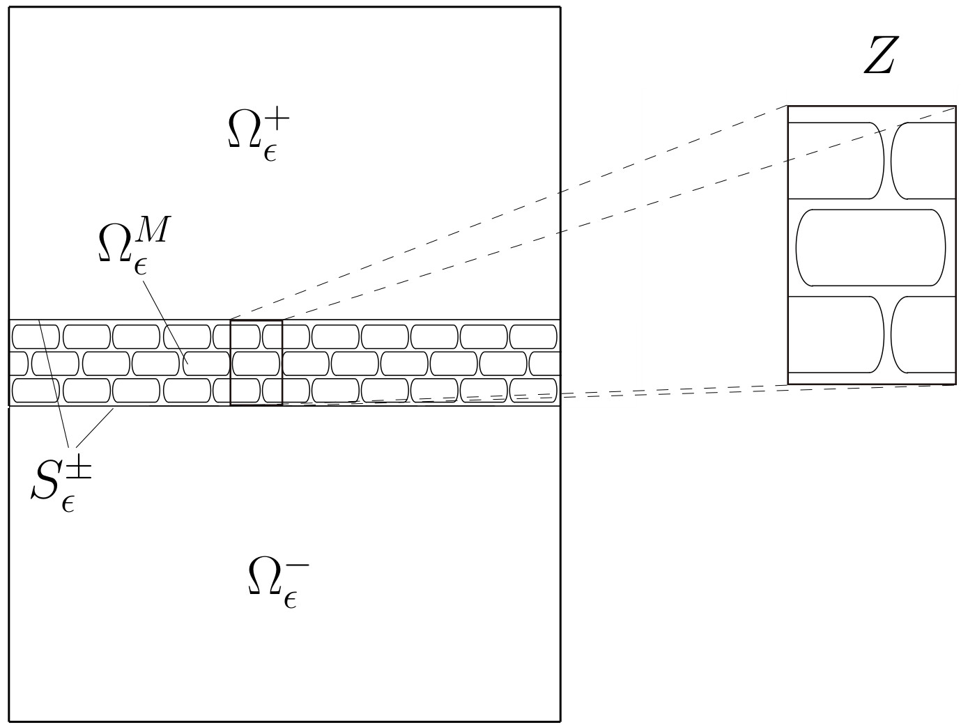 Figure 1
Peer Reviews
No public reviews on file for this paper yet. If you reviewed it on a platform where reviews are public (OpenReview, ICLR, NeurIPS, ICML), you can paste yours below so the community can read it here.
Videos
No videos yet. Explain this paper in a talk, walkthrough, or lecture? Add one.
Correctors and error estimates for reaction-diffusion processes through thin heterogeneous layers in case of homogenized equations with interface diffusion
M. Gahn Interdisciplinary Center for Scientific Computing, University of Heidelberg, Heidelberg, Germany. Mail: [email protected]
W. Jäger Interdisciplinary Center for Scientific Computing, University of Heidelberg, Heidelberg, Germany. Mail: [email protected]
M. Neuss-Radu Department of Mathematics, Friedrich-Alexander-Universität Erlangen-Nürnberg, Erlangen, Germany. *Mail: [email protected] *
Abstract
In this paper, we construct approximations of the microscopic solution of a nonlinear reaction–diffusion equation in a domain consisting of two bulk-domains, which are separated by a thin layer with a periodic heterogeneous structure. The size of the heterogeneities and thickness of the layer are of order , where the parameter is small compared to the length scale of the whole domain. In the limit , when the thin layer reduces to an interface separating two bulk domains, a macroscopic model with effective interface conditions across is obtained. Our approximations are obtained by adding corrector terms to the macroscopic solution, which take into account the oscillations in the thin layer and the coupling conditions between the layer and the bulk domains. To validate these approximations, we prove error estimates with respect to . Our approximations are constructed in two steps leading to error estimates of order and in the -norm.
Keywords: Asymptotic analysis; error estimates; correctors; boundary layers; reaction–diffusion equations; thin heterogeneous layer
MSC: 35B27; 35K57; 35C20
1 Introduction
Problems including reactive transport processes through thin layers with a heterogeneous structure play an important role in many applications, especially from biosciences, medical sciences, geosciences, and material sciences. We mention here as an example the physiological processes in blood vessels, where the endothelial layer, separating the lumen (region occupied by blood flow) from the vessel wall, mediates and controls the exchange between these two regions. In [32] a detailed model for processes at the endothelium is given by using phenomenologically derived effective interface laws. However, multi-scale techniques for the rigorous derivation of such laws starting from microscopic models, the study of their validity range and of the accuracy of the approximations are urgently needed. The techniques developed in this paper give an important contribution to this field, even though our model problem is limited to reaction–diffusion processes, and thus omitting further aspects like e.g. advective transport or mechano-chemical interactions.
In this paper, we consider a nonlinear reaction–diffusion equation in a domain consisting of two bulk-domains and which are separated by a thin layer with a periodic heterogeneous structure. The thickness of the thin layer as well as the period of the heterogeneities are of order , where the parameter is small compared to the length scale of the whole domain . Across the interfaces between the bulk-domains and the thin layer we assume continuity of the solution and its normal flux. The numerical computation of the solution to this type of problems faces a high complexity. Therefore, we construct approximations of the microscopic solution which can be calculated with less numerical effort, and prove error estimates between the approximation and the microscopic solution with respect to the scaling parameter . Such error estimates are important for the justification of the approximation as well as for predictions about its accuracy. There is a rich literature on problems in thin domains with applications in solid mechanics, wave diffraction, porous media and so on, where we have to mention the monographs [30] and [3]. Results about the derivation of effective transmission conditions by multi-scale techniques for domains separated by thin heterogeneous layers can be found e.g. in [4, 6, 7, 8, 11, 12, 14, 15, 23, 26, 29]. However, error estimates for thin heterogeneous layers coupled to bulk-domains have hardly been considered in literature so far. We mention here the paper [28], where an elliptic problem in a domain including a thin heterogeneous layer with thickness of order is treated for different scalings for the diffusion coefficients with respect to . More precisely, based on the Bakhvalov-ansatz the author derives higher order asymptotic approximations for the microscopic solution and derives error estimates with respect to . This method uses high regularity results for the microscopic and the macroscopic solutions, and therefore for the data. The asymptotic expansion is formally extended to nonlinear and nonstationary problems. In [1, 5, 22] the asymptotic behavior of a fluid flow through a filter formed by -periodic distribution of obstacles of size distributed on a hypersurface is considered and error estimates are proved. In [18] a similar geometrical setting was considered and the Poisson equation with mixed boundary conditions on the boundary of the obstacles was studied. In [31] a Neumann problem in a domain containing a thin filter consisting of periodically distributed channels is considered.
In [11, 12, 26] reaction-diffusion equations through thin heterogeneous layers were studied for different scalings in the thin layer, and effective models for were derived. In the singular limit, the thin layer reduces to a -dimensional interface separating the bulk-regions and . In these bulk-domains the evolution of the limit problem carries the same structure as in the microscopic problem, whereas at the interface effective interface laws emerge. Of particular importance is the choice of the scaling of the coefficients, especially in the equations in the thin layer. The scaling highly influences the structure of the macroscopic model and depends on the particular application.
In the present paper, we consider a specific scaling from [11] leading to a reaction-diffusion equation on the interface in the limit . This effective interface condition for the macroscopic model is similar to a result in [28] (see the interface condition (1.10)). However, in our case we consider a different scaling for the microscopic equation, and a nonlinear and nonstationary problem. Further, we consider a scaling for the reaction term in the thin layer which gives an additional contribution in the effective interface condition. For this situation, we investigate the quality of the approximation of the microscopic solution by means of the macroscopic one. In general, we cannot expect strong convergence of the gradients or high-order error estimates with respect to . For such results we have to add additional corrector terms to the macroscopic solution which take into account the oscillations in the thin layer and also the coupling conditions between the bulk-regions and the layer. The construction of the approximations is made in two steps. Firstly, we add to the macroscopic solution in the thin layer a corrector of order , which carries information about the oscillations in the layer. This leads to error estimates of order in the -norms, see Theorem 4. To obtain a better estimate, in a second step, we add a corrector term of first order to the macroscopic solutions in the bulk-domains (which equilibrates the discontinuity of the approximation across ) and an additional second order corrector to the macroscopic solution in the layer (which equilibrates the discontinuity of the normal fluxes of the approximation across ). This strategy of stepwise building up the correctors has also been used e.g. in [17]. The resulting approximation leads to an error estimate of order in the -norms, see Theorem 6.
The major challenge in our paper is the simultaneous scale transition for the thickness of the layer and the periodic heterogeneous structure within the layer, as well as the coupling between the bulk-domains and the thin layer, where we additionally have to take into account different kinds of scaling. In this context, the presence of nonlinear reaction terms creates additional difficulties. These specific features of our problem are also reflected by differences in the form of the correctors in the two regions (bulk domains and thin layer): The order of the corrector terms with respect to is different in the two regions. Furthermore, in the layer, the correctors are obtained by products of the derivatives of the macroscopic solution and solutions of suitable cell problems on a bounded reference element , whereas in the bulk-domains the correctors include solution of boundary layer problems in infinite stripes.
To justify the determined approximations, we prove error estimates. Roughly speaking, we apply the microscopic differential operator to the microscopic solution as well as to the approximations and subtract the terms from each other. To estimate the arising terms on the right hand side, the main idea is to represent solenoidal vector fields by the divergence of skew symmetric matrices. Integration by parts then yields an additional factor which can be exploited for the error estimates. This approach has been previously used in [19] for vector fields defined on the standard periodicity cell and periodic in all directions, and in [25] for boundary layers. In our case the situation is more difficult and we have to construct skew-symmetric matrices adapted to the structure of our problem. More precisely, these matrices have to be such that boundary terms which occur at the interfaces between the bulk domains and the thin layer vanish.
Our paper is structured as follows: In Section 2 we present the microscopic model, the assumptions on the data as well as the a priori estimates for the microscopic solution. In Section 3 we give the general form of the two approximations for the microscopic solution and state the corresponding error estimates. The macroscopic model and the higher order correctors are introduced in Sections 4 and 5 respectively. The proof for the error estimates is given in Section 6. We conclude the paper with a short appendix about the regularity of the solution to the macroscopic problem.
1.1 Original contributions
In the literature, there are several results dealing with singular limits for reactive transport processes through thin layers with heterogeneous structures. However, results including error estimates with respect to seem to be rather rare, especially with regard to nonlinear problems. In this paper we construct asymptotic approximations for the microscopic solution of a semilinear reaction-diffusion problem in a domain including a thin heterogeneous layer, and derive error estimates with respect to the scaling parameter . Besides providing control on the quality of the approximation, the correctors constructed by means of boundary layers have the suitable complexity to be used for numerical simulations (reducing the high complexity induced by the microstructure). The main contributions of our paper are:
the construction of approximations for the microscopic solution including correctors and boundary layers adapted to the scaling in the microscopic problem and the microscopic structure of the thin layer, as well as to the transmission conditions at the bulk-layer interfaces, 2. -
the derivation of error estimates of order and in the context of nonlinear problems which combine the classical approach of homogenization for microscopic structures with a singular limit approach, 3. -
proving of error estimates under low regularity assumptions on the data and therefore low regularity for the microscopic and the macroscopic solution, 4. -
extending the approach for the representation of solenoidal vector fields by the divergence of skew symmetric matrices to boundary layers involving transmission conditions.
2 The microscopic model
We consider the domain with fixed , , and with . Further, let be a sequence with . The set consists of three subdomains, see Figure 1, given by
[TABLE]
The domains and are separated by an interface , i. e.,
[TABLE]
hence, we have .
As mentioned above, for the membrane reduces to an interface , which we also denote by suppressing the -th component, and we define
[TABLE]
and . The microscopic structure within the thin layer can be described by shifted and scaled reference elements. We define
[TABLE]
We denote the upper and lower boundary of by
[TABLE]
Now, we consider a reaction-diffusion problem describing the evolution of a substance with concentration in the domain . Let with and be a solution of the following microscopic problem
[TABLE]
Here, and denote the diffusion coefficients of the substance in the bulk regions and in the thin layer respectively. The functions and model nonlinear reaction terms. Note that the heterogeneous structure of the thin layer is modeled by the oscillating diffusion coefficient and by the dependence of the reaction term on the microscopic variable .
In the following, we define for an arbitrary interval and a rectangle the Sobolev space of -periodic functions, i. e., the space of functions which are -periodic with respect to first components:
[TABLE]
for . In a similar way we also use the index for spaces with -periodic functions, e. g., .
Assumptions on the data:
- (A1)
It holds is symmetric and positive-definite, and with D^{M}\in C_{\#}^{0,1}\big{(}\overline{Z}\big{)}^{n\times n}. Further, is symmetric and coercive, i. e., there exists a constant such that
[TABLE] 2. (A2)
We have with is continuous, -periodic with respect to the second variable, and uniformly Lipschitz continuous with respect to the third variable. The uniform Lipschitz condition ensures the estimate
[TABLE] 3. (A3)
We have with is continuous, uniformly Lipschitz continuous with respect to the last variable, and -periodic with respect to the second variable. As above, we have
[TABLE]
Note that here, the variable describes the independent variable corresponding to the standard cell , and the variable corresponds to the dependent variable modeling the concentration . 4. (A4)
For the initial functions, we assume and with , and they fulfill the following estimate
[TABLE]
Further we assume that there exist and with , such that
[TABLE]
Weak formulation A function is called a weak solution of Problem , if for all , and almost every it holds that
[TABLE]
together with the initial condition .
To work on the fixed domains , we shift the -dependent domains to the fixed domains , and give an equivalent formulation for a weak solution on the fixed domains . We define
[TABLE]
Then is a weak solution of Problem , iff and with , and for all and with it holds that
[TABLE]
together with the initial condition
[TABLE]
Notation 1**.**
In the following, we suppress the and use the same notation for both, the shifted function, and the function itself.
We have the following existence and uniqueness result for the microscopic problem. A detailed proof can be found in [11], which can be easily extended to our slightly more general assumptions.
Proposition 2**.**
There exists a unique weak solution with and with of the Problem (satisfying the weak formulation ). Additionally, the following a priori estimates are valid:
[TABLE]
3 Main results
In this section we state our main results. We consider approximations of including correctors of first and second order, leading to different orders of convergence with respect to the scaling parameter . The definitions of the macroscopic solution of zeroth order and the corrector terms can be found in Section 4 and 5.
3.1 Correctors including terms of order in the layer
Let us define the first order approximation of by
[TABLE]
Remark 3**.**
The first order corrector term in the layer in the definition of takes into account the oscillations within the thin layer. Adding this corrector leads to a discontinuity of across the interfaces . Of course, it is also possible to add an additional first order corrector term in the bulk-domains (see the definition of below), however, this will not improve the order of convergence.
The error between the microscopic solution and the approximation is estimated in the following theorem:
Theorem 4**.**
Let with and , and with . Then, the following error estimate is valid
[TABLE]
and the constant fulfills
[TABLE]
Theorem 4 is a direct consequence of the more general result in Theorem 27 in Section 6.2.
3.2 Correctors including terms up to order in the layer
For higher order error estimates, we first have to overcome the problem of discontinuity across of the approximation by adding a first order corrector term in the bulk-domains, see Remark 3. However, this leads to an additional normal flux from the bulk-regions into the thin layer. Therefore, we have to add an additional second order corrector (the diffusion in the layer is of order ) in the layer. This leads to the following second order approximation: We define by
[TABLE]
Remark 5**.**
Again, the approximation is not continuous across the interfaces .
Theorem 6**.**
Let with , and with . Then, the following error estimate is valid
[TABLE]
and the constant fulfills
[TABLE]
We see that the second order approximation leads to a better error estimate with respect to the scaling parameter than . However, from the numerical point of view, this has to be paid by solving the cell and boundary layer problems for the correctors and , see Section 5.
4 The zeroth order macroscopic model
In this section we formulate the macroscopic problem of zeroth order. This was derived rigorously for a similar model in [11] using the method of two-scale convergence and the unfolding operator. Here, we also take into account oscillations in the reactive term and consider periodic boundary conditions on the lateral boundary instead of a Neumann-zero boundary condition. However, the results from [11] still hold for our situation.
The macroscopic solution is defined in the following way: Let the triple with
[TABLE]
be the unique weak solution of the following transmission problem:
[TABLE]
with [\![D^{\pm}\nabla c_{0}^{\pm}\cdot\nu]\!]:=-\big{(}D^{+}\nabla c_{0}^{+}\cdot\nu^{+}+D^{-}\nabla c_{0}^{-}\cdot\nu^{-}\big{)}. Here, denotes the outer unit normal on , and the homogenized diffusion coefficient is defined by
[TABLE]
where are the solutions of the cell problems in Section 5. The variational formulation for Problem is the following one: For all with it holds almost everywhere in
[TABLE]
In the following we will prove regularity results for the macroscopic solution under additional assumptions on the data. Hence, let the Assumptions (A1) - (A4) be valid and additionally it holds that
- (A2)’
The function is differentiable with respect to with . 2. (A3)’
The function is differentiable with respect to with . 3. (A4)’
There exists a constant , such that (not for the -th derivative) and .
Then we obtain the following regularity result for the macroscopic solution, which is sufficient for the assumptions in Theorem 4 and 6 to hold:
Proposition 7**.**
Let the conditions (A1) - (A4) be fulfilled. Then the triple has the following regularity property:
[TABLE]
If we additionally assume (A2)’ - (A4)’, then we obtain
[TABLE]
Proof.
The proof can be found in Section A in the Appendix. ∎
Remark 8**.**
We emphasize that the proofs of the main results from Section 3 hold under the Assumptions (A1) - (A4), and the conditions stated in Theorem 4 and 6. The assumptions (A2)’ - (A4)’ give sufficient conditions for which the assumptions from Theorem 4 and 6 are fulfilled, but are far away from being optimal.
5 Corrector terms
In this section we define the corrector terms , , and used in the first and second order approximations and in Section 3, and investigate their regularity properties. The correctors are defined via the derivatives of the macroscopic solution multiplied by solutions of appropriate cell respectively boundary layer problems, see - .
**Cell problems of first order for the thin layer : **
For the function solves the following cell problem:
[TABLE]
Lemma 9**.**
For every there exists a unique solution of Problem for arbitrary large. Especially, we have
[TABLE]
Proof.
This follows from the -theory for the Neumann-problem for elliptic equations, see [16, Chapter 2]. The inequality follows from the Sobolev embedding theorem for . ∎
Now, we define the first order corrector in the thin layer via
[TABLE]
By adding to the macroscopic solution in the thin layer, we take into account the oscillations in the layer and can prove error estimates for the gradients in , see Theorem 4.
Boundary layer corrector for the bulk-domains :
Using the corrector , we obtain an error estimate of order , see Theorem 4. To obtain a better error estimate, we add further corrector terms to the approximation . Firstly, we add the corrector to the macroscopic solution in the bulk domains, which eliminates the discontinuity across the interfaces of the approximation .
Let us define the infinite stripes and their interface by
[TABLE]
For fixed , we define
[TABLE]
and in the same way we define the space W_{\omega,\#}\big{(}Y^{-}\big{)}. For , the function w_{j,1}^{\pm,\mathrm{bl}}\in W_{\omega,\#}\big{(}Y^{\pm}\big{)} solves the following boundary layer problem
[TABLE]
Lemma 10**.**
For every , there exists a unique solution for a suitable . Additionally, it holds that w_{j,1}^{\pm,\mathrm{bl}}\in W^{2,p}_{\mathrm{loc}}(\mathbb{R}^{n}_{\pm})\cap C^{0}\big{(}\overline{\mathbb{R}^{n}_{\pm}}\big{)} with for arbitrary large . Especially, we have for a constant
[TABLE]
Proof.
The existence and uniqueness follows from [21, Theorem 10.1] and the regularity result from Lemma 9. The local -regularity follows from the -theory for elliptic equations, which also implies the continuity of the solution. It remains to check that the solution and its gradient are bounded on . This follows from the weak maximum principle, see [24, Theorem A.1.1] and also [13, Section 8.1]. More precisely we have
[TABLE]
Now, the local estimate from [13, Theorem 9.11] which holds uniformly on every ball with fixed radius in and the Morrey inequality imply the boundedness of the gradient. ∎
We define the first order corrector term for the bulk-domains by
[TABLE]
Here, we take with and in a neighborhood of [math]. Now, the functions and coincide on the interfaces .
Corrector of second order for the thin layer :
The corrector leads to a jump of the normal fluxes across . Therefore, we add an additional corrector of second order in the thin layer. We emphasize that due to the different scaling of the diffusion coefficients in the bulk-domains and the thin layer in the microscopic problem, we can expect correctors of different orders in the bulk domains and the layer.
For the function solves the following cell problem:
[TABLE]
Lemma 11**.**
For , there exists a unique solution of Problem for arbitrary large . Especially, we have
[TABLE]
Proof.
Again, the claim follows from the -theory for the elliptic equations with Neumann-boundary conditions, and the regularity results from Lemma 10. ∎
We define the second order corrector in the thin layer by
[TABLE]
6 Error estimates
In this section, we give the proof of our main results. Roughly speaking, the idea is to apply the microscopic differential operator from Problem to the microscopic solution and the approximative solution (), and subtract these terms from each other. More precisely, we start from the following term: For and with we consider for
[TABLE]
where we use the short notation . At this point, we do not give precise information about the regularity of the macroscopic solution . This will be specified in the following results. Our aim is to estimate the terms in and to choose a suitable test function. However, as mentioned in Remark 3 and 5, the error function is not an admissible test function. Therefore, we have to add an additional corrector term in the bulk-domains, what leads to an additional error.
We estimate the terms in for , because the most error terms carry over to the case . First of all, by using we obtain
[TABLE]
For the last term , an elemental calculation gives
[TABLE]
Let us define the tensor by
[TABLE]
for and . This gives us (we consider as both, a vector in and in with the last component equal to zero)
[TABLE]
With similar arguments and by adding in a suitable way, we obtain for by using and (if it is necessary, we consider as an element of by setting the -th row and column equal to zero):
[TABLE]
with
[TABLE]
defined for and by
[TABLE]
Now, let us define the averaged function by
[TABLE]
We observe that with this definition we can write
[TABLE]
Altogether, we obtain for the term :
[TABLE]
with
[TABLE]
and
[TABLE]
We emphasize that is an admissible test function for the variational equation of the microscopic problem, but is not an admissible test function for the variational equation of the macroscopic model of zeroth order. Therefore, in the following we use equation tested with \big{(}\phi_{\epsilon}^{\pm},\overline{\phi}_{\epsilon}^{M}\big{)}. Due to the regularity of from Proposition 7, the normal fluxes are elements of . Hence, from and we obtain
[TABLE]
We have to estimate the terms on the right-hand side, where the most challenging term is . We start with , which only occurs for .
Lemma 12** (Estimate for ).**
For and , for almost every it holds that
[TABLE]
Proof.
The estimate follows easily from the Hölder-inequality and the essential boundedness of and , see Lemma 9 and 10. ∎
Remark 13**.**
Here we use the additional regularity for the time derivative of the macroscopic solution from the hypothesis in Theorem 6.
Lemma 14** (Estimate for ).**
For and , for almost every it holds that
[TABLE]
Proof.
The claim follows easily from the continuity of and the regularity results from Lemma 9, 10 and 11. ∎
Lemma 15** (Estimate for the interface term in ).**
Let . Then almost everywhere in it holds that
[TABLE]
Proof.
The fundamental theorem of calculus and imply
[TABLE]
Now, the regularity of implies
[TABLE]
∎
Estimates for the nonlinear terms in :
Let us estimate now the differences including the nonlinear terms in . We start with the following auxiliary Lemma:
Lemma 16**.**
Let and let us define by
[TABLE]
There exists for arbitrary large, such that
[TABLE]
Especially, the following estimate holds:
[TABLE]
Proof.
Here, the time variable has the role of an additional parameter and for an easier notation we suppress the time-dependence in the following.
Step 1* (Existence of a solution ): *First of all, the function is an element of , since we obtain from the growth condition from Assumption (A3)
[TABLE]
Further, the mean value with respect to is obviously zero. Additionally, the regularity of implies
[TABLE]
for and almost every . Since the derivative of a Lipschitz-function is bounded (independent of , due to our assumptions), we obtain
[TABLE]
i. e., . Now, let be the unique solution of the following problem:
[TABLE]
The -theory for elliptic equations implies for arbitrary, and
[TABLE]
To prove regularity of with respect to , we use the method of difference quotients, see [13, Section 7.11]. We define for , , and the difference quotient by
[TABLE]
with . Then, is a solution of
[TABLE]
By the same arguments as above we obtain and
[TABLE]
The results from [13, Section 7.11] extended to Banach valued functions implies . Especially, we can replace in the problem above by .
Now, we define . This gives us the desired result for , where the estimate follows from the continuous embedding W^{1,p}(Z)\hookrightarrow C^{0}\big{(}\overline{Z}\big{)}.
Step 2* (Periodicity of with respect to )*: We define the space of -functions on with mean value zero by . Further, let or , and we define the linear operator
[TABLE]
where is the unique weak solution of
[TABLE]
Existence and uniqueness follows as in Step 1 from the Lax-Milgram Lemma, which also implies the continuity of the operator . We consider the following vector-valued trace operators (see [2, Theorem 6.13])
[TABLE]
The claim is proved, if we show
[TABLE]
With similar arguments as in Step 1, we obtain the regularity result
[TABLE]
hence, the identity holds on . The density of and the continuity of and the trace operators imply the desired result. ∎
Proposition 17**.**
Let . Then it holds that
[TABLE]
Proof.
We have
[TABLE]
For the first term we use the uniform Lipschitz continuity of to obtain
[TABLE]
For the second term we use Lemma 16 to obtain
[TABLE]
The last term vanishes, due to the periodicity of and on . Further, the estimate from Lemma 16 implies
[TABLE]
In a similar way, we can estimate . ∎
Proposition 18**.**
Let . Then it holds that
[TABLE]
Proof.
We argue in the same way as in the proof of Proposition 17. We have
[TABLE]
where for arbitrary large fulfills (we again suppress the time-dependence)
[TABLE]
and the estimate
[TABLE]
The existence and the regularity of can be established in the same way as in Lemma 16. However, we emphasize that we do not require specific boundary conditions for on . We obtain
[TABLE]
We only consider the boundary term in more detail. The vector valued trace inequality implies
[TABLE]
∎
Estimate for
Now, we estimate the term , where according to we use the following notations for the included terms:
[TABLE]
The mean idea is to represent solenoidal vector fields by the divergence of skew-symmetric matrices and integrate by parts. This gives an additional factor . This approach has been used in [19, Section 4.2] for vector fields on , periodic in all directions, and [25] for boundary layers. In our case, we have to construct skew-symmetric matrices adapted to the structure of our problem. More precisely, these matrices have to be such that boundary terms which occur at the interfaces between the bulk domains and the thin layer vanish.
We start with the estimate for the term . Therefore, we make use of the following Lemma:
Lemma 19**.**
Let for with
[TABLE]
This means, that for all which are -periodic ( the dual exponent of ) it holds that
[TABLE]
Then, there exists a skew-symmetric tensor \big{(}\beta_{il}\big{)}\in W^{1,p}(Z)^{n\times n} for , such that
[TABLE]
Proof.
We define
[TABLE]
where is the solution of
[TABLE]
From the -theory for elliptic equations we obtain and therefore . Obviously, the boundary conditions for on imply . Further, we have
[TABLE]
where we defined . We show that . First of all, we have is -periodic and
[TABLE]
due to the zero-boundary condition of on . Further, for all -periodic \phi\in C^{\infty}\big{(}\overline{Z}\big{)} we have
[TABLE]
For the second term we obtain from the properties of and the definition of
[TABLE]
Further, the periodicity and the Dirichlet-zero boundary condition of imply
[TABLE]
Using the Neumann-boundary conditions for for , we get by similar arguments
[TABLE]
Altogether, we obtain
[TABLE]
and therefore satisfies
[TABLE]
This implies and the proof is complete. ∎
Lemma 20**.**
Let . Then it holds that
[TABLE]
Proof.
We have
[TABLE]
Let us define for fixed the function by . An elemental calculation shows that fulfills the assumptions of Lemma 19. Hence, there exists for every a skew symmetric tensor \big{(}\beta_{jl}^{i}\big{)}\in W^{1,p}(Z) (for arbitrary large), such that in and on . This implies by integration by parts
[TABLE]
The boundary term vanishes due to the boundary conditions of and on the lateral boundary, and the boundary condition of on . The terms including the derivatives vanish due to the skew-symmetry of and the symmetry of the Hesse-matrix of . Then, the regularity of implies
[TABLE]
∎
It remains to estimate the term . First of all we define for
[TABLE]
and the space
[TABLE]
where denotes the space of functions belonging to for every such that is compact. In a similar way we define other Sobolev spaces which are integrable locally on . For we define the mean value of over for by
[TABLE]
On we have the following weighted Poincaré-type inequality (see [17, Prop. 1.3])
[TABLE]
Therefore, the space
[TABLE]
becomes a Hilbert space with respect to the inner product
[TABLE]
Lemma 21**.**
Let with for . Then there exists a unique weak solution of the problem
[TABLE]
Proof.
The proof is based on the inequality and can be found in [17, Prop. 1.5]. ∎
Next we show additional regularity results for the solution from Lemma 21 under additional assumptions on . We use similar methods as in [17, 27]. However, for the sake of completeness we give the detailed proof for our case.
Lemma 22**.**
For let , , and for such that for every it holds that
[TABLE]
with a constant independent of . Then the solution from Lemma 21 fulfills with uniformly with respect to . Especially we have and .
Proof.
The -theory of elliptic operators implies . Now, we prove ()
[TABLE]
In fact, let and with , in , in , and . Then by testing with and integrating over , we obtain
[TABLE]
since . Using again the equation , we get for
[TABLE]
Integration with respect to from [math] to implies ()
[TABLE]
for a constant independent of . Now, the Poincaré-inequality implies for every
[TABLE]
The same arguments hold for , what implies . The claim follows from Theorem 8.17, 9.11, and 8.32 from [13]. ∎
Now we are able to construct the skew-symmetric tensors corresponding to the error terms and .
Lemma 23**.**
For let and for such that holds for all , and
[TABLE]
More precisely, the conditions and is -periodic means that for all it holds that
[TABLE]
Then there exists a -periodic, skew symmetric tensor \big{(}\beta_{kl}\big{)}\in L^{2}(Z_{\infty})\cap W^{1,p}_{\mathrm{loc}}(\overline{Z_{\infty}})\cap C^{0}(\overline{Z_{\infty}}), such that
[TABLE]
Proof.
From Lemma 21 we obtain the existence of a function such that in . Now, we define for . The regularity of follows immediately from Lemma 22 and we only have to check the claim that holds. The definition of implies (as in the proof of Lemma 19)
[TABLE]
with and . Then, follows if we show .
First of all, for we define and with , in , and . For every we obtain
[TABLE]
The boundary terms vanish, due to the periodicity of and , as well as the compact support of in . Using and , we get
[TABLE]
By a density argument this result is also valid for , and we obtain for from the monotone convergence theorem:
[TABLE]
It remains to show for . We illustrate this for one term in . From the Hölder-inequality we obtain
[TABLE]
This proves the claim. ∎
Lemma 24**.**
Let and . Then it holds that
[TABLE]
Proof.
We proceed in a similar way as in Lemma 20, whereby we now use Lemma 23. Here, the crucial point is to control the boundary terms on , which occur by replacing and by skew-symmetric tensors and integrating by parts. We handle this by constructing skew-symmetric tensors which are continuous across .
First of all, we fix and define for
[TABLE]
We show that fulfills the conditions of Lemma 23 except the mean value condition. The properties of (see Lemma 10) imply the integrability conditions on from Lemma 23 (remember that we can choose arbitrary large, especially ). Further, according to , we have in and by we have in . The Neumann-boundary condition of on implies on , where denotes the outer unit normal on with respect to . Hence, we obtain on . Now we show, that fulfills the mean value condition:
For every with and it holds that
[TABLE]
We emphasize that the trace of exists, due to the regularity of and . Since is arbitrary, we obtain
[TABLE]
Let us check that this term is equal to zero. Let (the case follows the same lines) and with , , and in an neighborhood of . From the exponential decay of we immediately obtain
[TABLE]
Since is divergence-free, we obtain
[TABLE]
This implies for all . Especially, we obtain .
For arbitrary we define by in and in . Then, for we still have in and fulfills the same integrability conditions as . We choose in such a way that for . Then, Lemma 23 implies the existence of a skew-symmetric tensor \big{(}\beta_{jl}^{i}\big{)}\in W^{1,p}_{1,\#}(Z_{\infty}) with .
Now, we consider the error terms and . We have
[TABLE]
For the second term we immediately obtain from the Hölder-inequality
[TABLE]
For the first term we obtain by integration by parts
[TABLE]
where the lateral boundary terms of vanish, due to the -periodicity of the functions, and the terms involving vanish, due to the skew-symmetry of . With similar arguments, we obtain
[TABLE]
Adding up these terms, the boundary terms cancel out and we obtain
[TABLE]
Now, using the essential boundedness of from Lemma 23, we obtain the desired result. ∎
We summarize our results in the following proposition:
Proposition 25**.**
For with and with the following estimate is valid for all and with :
[TABLE]
Proof.
For smooth functions and the result follows directly from and , Proposition 17 and 18, and Lemma 12, 14, 20, 24, and 15. Then, the result for functions and follows by a density argument. ∎
6.1 Error estimates for the first order approximation
In this subsection, we give the proof of Theorem 4, i. e., we proof the estimate for the error . We start from equation with and use the same methods as for equation . Then for all and with , we get
[TABLE]
with
[TABLE]
Lemma 26**.**
Let , then for the first order corrector in the bulk-domains it holds that
[TABLE]
Especially, we have
[TABLE]
with .
For , the first order corrector in the thin layer fulfills
[TABLE]
Especially, we have
[TABLE]
with .
Proof.
These estimates easily follow from the regularity results for and in Lemma 11 and 9, and the a priori estimates in Proposition 2. ∎
Theorem 27**.**
Let with and , and with . Then, the following error estimate is valid
[TABLE]
Proof.
We already mentioned that is not an admissible test function for , hence, we add the corrector term in the bulk-domains to obtain the admissible test function
[TABLE]
We use this test function in the equation and obtain
[TABLE]
Using the coercivity of and , we get for a constant
[TABLE]
From Proposition 17 and 18, and Lemma 14, 15, and 20 we obtain
[TABLE]
Integration with respect to time and Lemma 26 yields for almost every
[TABLE]
For and , we immediately obtain from the Hölder-inequality
[TABLE]
For we obtain
[TABLE]
By a change of variables and the -periodicity of , we obtain
[TABLE]
The term including can be estimated in the same way. Now, for every there exists a constant , such that for all it holds that . This implies
[TABLE]
For , the last term on the right-hand side can be absorbed from the left-hand side in . Integration of with respect to time, Gronwall-inequality, and Lemma 26 imply
[TABLE]
The a priori estimates from Proposition 2 and Assumption (A4) imply the desired result. ∎
As a direct consequence, we obtain Theorem 4:
Proof of Theorem 4.
This follows directly from Theorem 27 and Lemma 26. ∎
6.2 Error estimates for the second order approximation
As in the case of the first order approximation, we have the problem that is not an admissible test function, because it is not continuous across (after a shift back to the domain ). We have to add a corrector to the bulk-approximation with . Therefore, we define
[TABLE]
i. e., we extend the trace of on constant to the infinite strip and multiply it by the cut-off function , which was defined in Section 5. The regularity of and the trace embedding from [33, Remark 4, Section 2.9.1] imply , and the Hölder-embedding [33, Theorem 4.6.1(e)] implies that and are essential bounded, i. e., we have
[TABLE]
Now, we define
[TABLE]
Lemma 28**.**
Let with . Then, for the correctors and in the bulk-domains it holds that
[TABLE]
For with , the correctors and in the thin layer fulfill the following inequalities
[TABLE]
Proof.
We only give the proof for . From the essential boundedness of and , we immediately obtain
[TABLE]
∎
Theorem 29**.**
Let with and with . Then, the following error estimate is valid
[TABLE]
Proof.
We start from the inequality from Proposition 25 and choose as a test function
[TABLE]
Let us denote by the terms on the right-hand side in the inequality . Then, the coercivity of and implies for a constant after integration with respect to time that for almost every it holds that
[TABLE]
Here, includes all terms containing initial values. Let us estimate the terms on the right-hand side. Some elemental calculations and the estimates from Proposition 2 and Lemma 26 and 28 give us (we emphasize that these equations are valid pointwise in time)
[TABLE]
These estimates imply (together with the inequality ) almost everywhere in
[TABLE]
Using again Proposition 2 and Lemma 26 and 28, we obtain for almost every
[TABLE]
It remains to estimate the initial term . Assumption (A4) and (A4)’, the regularity of and , Lemma 26, and the essential boundedness of and imply
[TABLE]
Plugging in these estimates in , we obtain the desired result. ∎
As an immediate consequence we obtain Theorem 6.
Proof of Theorem 6.
This is a direct consequence of Theorem 29 and Proposition 2. ∎
Remark 30**.**
**
- (i)
Our results are not restricted to the Assumptions (A2) - (A4), and (A2)’ - (A4)’. In fact, the error estimates from Theorem 4 and 6 remain valid, if the microscopic solution fulfills the a priori estimates from Proposition 2, the nonlinear functions fulfill the estimates from Proposition 17 and 18, the initial values fulfill the error estimate , and the macroscopic solution fulfills the regularity hypothesis from Theorem 4 and 6. 2. (ii)
Theorem 27 and therefore Theorem 4 still hold if we replace the condition in Assumption (A4) by the weaker condition
[TABLE]
This can be easily seen from the last inequality in the proof of Theorem 27. In this case the error for the second order approximation is also of order , i. e., no better error estimate is obtained by using the improved approximation .
7 Conclusion and outlook
In our paper, we derived approximations of order and for the microscopic solution of the microscopic model describing nonlinear and nonstationary reaction-diffusion processes in media separated by thin periodically heterogeneous layers. The approximations are constructed via the solution of the macroscopic model and additional correctors including solution of cell problems and boundary layers. The challenging aspects are related to the simultaneous scale transition for the thickness of the layer and the periodicity within the layer, the coupling between the bulk domains and the thin layer, and the nonlinear reaction kinetics.
Using the iterative procedure of our paper, it is possible to construct approximations of higher order. However, in the general setting considered in this paper it is not possible to obtain higher order error estimates. First of all, the oscillations in the reaction-kinetics lead to an error of order (even if the reaction term is independent of the solution). If we consider nonlinear reaction-kinetics independent of the oscillating variable, we need additional regularity for the nonlinear functions (Taylor-expansion) to perform the asymptotic expansion. In our applications, however, see e.g., [10], where Michaelis-Menten-type kinetics are required, we can only expect to have Lipschitz regularity. Last but not least, due to different geometrical structures present in the microscopic and the macroscopic model (the thin layer reduces to a lower dimensional interface), we obtain an approximation error of order , see Lemma 15, and it is not clear how this error can be reduced further. We emphasize that in our proof the derivation of the -error and the -error go hand in hand, hence it is not possible to improve the -error.
In this paper we only considered the case of high diffusion in the thin layer, i.e., the diffusion coefficient in the layer is of order . Here, the limit solution in the layer does not depend on the microscopic variable . This is also the case for moderate diffusion, when , see [11]. However, in this case the diffusion term in the homogenized problem in the layer vanishes and the homognized solution in the layer satisfies an ordinary differential equation. In the case of very small diffusion, when , see [26], the macroscopic model depends on both, the microscopic variable and the macroscopic variable . This completely different structure of the macroscopic problem in the case compared to the cases does not permit to derive error estimates by the methods developed in this paper directly. On the other hand, for the case , we see the possibility to add an additional term in the macroscopic equation at the interface , namely
[TABLE]
to obtain a reaction-diffusion equation on , as in the case considered in this paper:
[TABLE]
Then we can use the same methods as above and expect error estimates depending on , and getting worse in the critical limit . However, this is part of ongoing work.
Appendix A Regularity proofs for the macroscopic solution
In this section, we give the proof of the regularity results in Proposition 7 without going into detail. We shortly write:
[TABLE]
and
[TABLE]
Further we define for and , and given and the sets
[TABLE]
The following technical lemma is an extension of [20, Chapter II, Theorem 6.1] for our geometrical setting:
Lemma 31**.**
Let , , , and assume that there exist and , such that for all it holds that
[TABLE]
for and (here for ). Then, we have
[TABLE]
Proof.
The proof can easily be adapted from [20, II, Theorem 6.1] and is skipped here. ∎
Proof of Proposition 7.
First of all, we obtain and by testing with the difference quotient of with respect to the spatial variable for the -th component with ( can be extended periodically to ). For more details, we refer to [11, Lemma 2.4].
The regularity and is formally obtained by differentiating the problem with respect to time. Rigorously, this can be done by a priori estimates for a Galerkin approximation. For more details we refer to [9]. Here, we make use of the differentiability of and with respect to from the additional assumptions (A2)’ and (A3)’, as well as the essential boundedness of and from (A4)’.
It remains to check the essential boundedness of and . Formally this can be done by differentiating the equation with respect to for . Let us do this in a more rigorous way, where the ideas can be found in [20]. As test functions in , we choose and with and and . Then, by integration by parts we obtain with the periodic boundary conditions on the lateral boundary and the regularity results from above the following weak formulation for and
[TABLE]
together with the initial condition and (this is exactly the weak formulation we obtain by formally differentiating with respect to ). By density, see [11, Lemma 5.3], this equation is valid for all with . For (see (A4)’), we choose and with and obtain by an elemental calculation using the essential boundedness of and (which follows from the uniform Lipschitz continuity with respect to ), the estimate (for a constant )
[TABLE]
Integration with respect to time, the condition (A4)’, and the Gronwall inequality imply
[TABLE]
An application of Lemma 31 with and gives the desired result. ∎
Acknowledgment
The authors acknowledge the support by the Center for Modelling and Simulation in the Biosciences (BIOMS) of the University of Heidelberg. The first author was supported by the project SCIDATOS (Scientific Computing for Improved Detection and Therapy of Sepsis), which was funded by the Klaus Tschira Foundation, Germany (Grant number 00.0277.2015).
The reference list from the paper itself. Each links out to its DOI / PubMed record.
- 1[1] G. Allaire. Homogenization of the Navier-Stokes equations in open sets perforated with tiny holes II: Non-critical sizes of the holes for a volume distribution and a surface distribution of holes. Arch. Rational Mech. Anal. , 113:261–298, 1991.
- 2[2] W. Arendt and M. Kreuter. Mapping theorem for Sobolev-spaces of vector-valued functions. Studia Math. 240 , 3:275–299, 2018.
- 3[3] N. S. Bakhvalov and G. Panasenko. Homogenisation: Averaging Processes in Periodic Media . Kluwer Academic Publishers, 1989.
- 4[4] A. Bourgeat, O. Gipouloux, and E. Marušić-Paloka. Modelling of an underground waste disposal site by upscaling. Math. Meth. Appl. Sci. , 27:381–403, 2004.
- 5[5] A. Bourgeat, S. Marušić, and E. Marušić-Paloka. Écoulement non newtonien à travers un filtre mince. Comptes Rendus de l’Académie des Sciences-Series I-Mathematics , 324(8):945–950, 1997.
- 6[6] A. Bourgeat and E. Marušić-Paloka. A homogenized model of an underground waste repository including a disturbed zone. Multiscale Model. Simul. , 3(4):918–939, 2005.
- 7[7] C. Conca. Étude d’un fluid traversant une paroi perforeé I. Comportement limite près de la paroi. J. Math. pures et appl. , 66:1–43, 1987.
- 8[8] C. Conca. Étude d’un fluid traversant une paroi perforeé II. Comportement limite loin de la paroi. J. Math. pures et appl. , 66:45–69, 1987.