Linear Convergence of Primal-Dual Gradient Methods and their Performance in Distributed Optimization
Sulaiman A. Alghunaim, Ali H. Sayed

TL;DR
This paper proves the linear convergence of primal-dual gradient methods for smooth strongly-convex problems and analyzes how augmented Lagrangian penalties affect distributed optimization performance.
Contribution
It provides a concise proof of exponential convergence and explores the impact of augmented Lagrangian terms in distributed settings.
Findings
Proves linear convergence of primal-dual gradient methods for strongly-convex functions.
Analyzes the effect of augmented Lagrangian penalties on distributed optimization.
Relates incremental and non-incremental implementations of the algorithm.
Abstract
In this work, we revisit a classical incremental implementation of the primal-descent dual-ascent gradient method used for the solution of equality constrained optimization problems. We provide a short proof that establishes the linear (exponential) convergence of the algorithm for smooth strongly-convex cost functions and study its relation to the non-incremental implementation. We also study the effect of the augmented Lagrangian penalty term on the performance of distributed optimization algorithms for the minimization of aggregate cost functions over multi-agent networks.
Click any figure to enlarge with its caption.
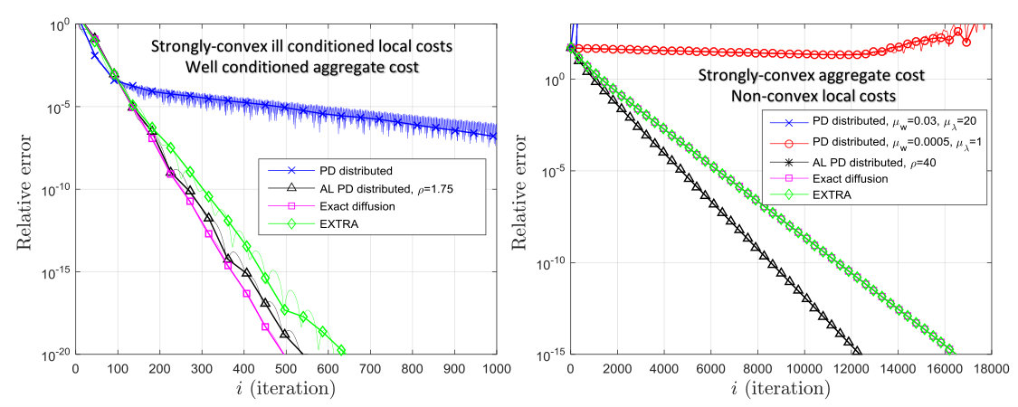 Figure 1
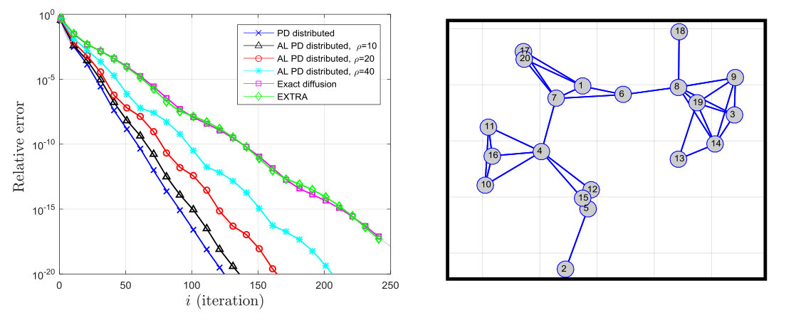 Figure 2
Peer Reviews
No public reviews on file for this paper yet. If you reviewed it on a platform where reviews are public (OpenReview, ICLR, NeurIPS, ICML), you can paste yours below so the community can read it here.
Videos
No videos yet. Explain this paper in a talk, walkthrough, or lecture? Add one.
Linear Convergence of Primal-Dual Gradient Methods and their Performance in Distributed Optimization
Sulaiman A. Alghunaim*∗* and Ali H. Sayed*†, Fellow, IEEE This work was supported in part by grant 205121-184999 from the Swiss National Science Foundation.∗*S. A. Alghunaim is with the ECE Department, University of California at Los Angeles (UCLA). Email:[email protected]. *†*A. H. Sayed is with the Ecole Polytechnique Federale de Lausanne EPFL, School of Engineering, CH-1015 Lausanne, Switzerland e-mail: [email protected].
Abstract
In this work, we revisit a classical incremental implementation of the primal-descent dual-ascent gradient method used for the solution of equality constrained optimization problems. We provide a short proof that establishes the linear (exponential) convergence of the algorithm for smooth strongly-convex cost functions and study its relation to the non-incremental implementation. We also study the effect of the augmented Lagrangian penalty term on the performance of distributed optimization algorithms for the minimization of aggregate cost functions over multi-agent networks.
Index Terms:
Primal-dual methods, linear convergence, Arrow-Hurwicz, augmented Lagrangian, distributed optimization.
I Introduction
Consider the constrained optimization problem:
[TABLE]
where is a smooth function assumed to satisfy Assumption 1 further ahead, , and . Consider also the saddle point problem:
[TABLE]
where
[TABLE]
is the augmented Lagrangian of problem (1), is a dual variable, and is the augmented Lagrangian penalty parameter. Note that for , becomes the classical Lagrangian of problem (1). If a point exists that solves (2), then is an optimal solution to the constrained problem when strong duality holds, which is the case under our assumptions [1]. A classical algorithm that solves (2) is the primal-dual (PD) gradient algorithm (4). In this algorithm, denotes the gradient of evaluated at and are positive step-sizes (learning rates) chosen by the designer. The updates in (4) are primal-descent dual-ascent steps applied to (3) and it subsume the classical Lagrangian implementation when and the augmented Lagrangian implementation when . Note that the updates in (4) are incremental since the dual update (4b) uses the most recent primal variable and not . If the dual update uses the previous primal iterate , then we refer to the update as non-incremental.
This work provides a concise proof that establishes the linear convergence of recursion (4) and studies its relation to the non-incremental implementation. We also study the effect of the penalty term on the performance of multi-agent consensus optimization algorithms. Algorithms of the form (4) have been applied in various applications including wireless systems [2], power systems [3], reinforcement learning [4], and network utility maximization [5].
I-A Related Works
There exists a large body of literature on primal-dual saddle-point algorithms – see [6, 7, 8, 9, 10, 11, 5, 12, 13] and the references therein, including the seminal work [6], which proposed recursions of the type (4) and established their convergence. These works focus on proving convergence to an optimal solution without providing convergence rates, provide sub-linear convergence rates (e.g., where is the iteration index), or show linear convergence from a starting point that is sufficiently close to a solution (local convergence). Some other works examined global linear convergence under different settings.
The works [14, 15] focuses on continuous versions of the primal-dual gradient dynamics and establish linear convergence for augmented Lagrangian implementations (i.e., they require the presence of the augmented Lagrangian term , where is strictly positive). They also require to have full row rank. Similarly, the work [16] establishes linear convergence for continuous primal-dual gradient dynamics for full row rank , but it does not require the presence of the augmented Lagrangian term. Moreover, it was shown in [16] that if the continuous dynamics is discretized using Euler discretization, then the discrete version converges linearly under small enough step sizes. However, no upper bound is given on the step-sizes. Moreover, Euler discretization uses identical step-sizes for the primal and dual updates (i.e., ) and results in a non-incremental primal-dual dynamics. Therefore, the results in [14, 15, 16] are not directly applicable to the discrete incremental implementation (4) and do not provide clear bounds on the step-sizes.
We remark that linear convergence for various monotone operator methods have been established albeit under other conditions that are not satisfied in our setup. For example, the linear convergence results in [17] and [18, Proposition 25.9] for forward-backward splitting methods would require the saddle-point problem (2) to be both strongly-convex with respect to and strongly-concave with respect to . This holds for example for problems with Lagrangian where and are both strongly-convex functions. Similarly, the conditions used in [19, 20, 21] require the saddle-point problem (2) to be strongly-convex with respect to and strongly-concave with respect to . In our setup, is not strongly-concave with respect to .
The work [22] showed that for saddle point problems with , linear convergence is possible without requiring the Lagrangian to be both strongly-convex and strongly-concave. In particular, it established linear convergence when the primal function is smooth and convex, the dual function is smooth and strongly-concave, and the additional assumption that is a full column rank matrix. Unlike the current work, the algorithm analyzed in [22] is non-incremental; moreover, particular fixed step-sizes are needed to establish linear convergence – [22, Theorem 3.1].
Now, in the distributed optimization literature, various incremental primal-dual gradient algorithms have been proposed to solve multi-agent consensus optimization problems – see [23, 24, 25, 26, 27] and references therein, which are mostly based on AL formulations. They have been shown to achieve linear convergence under strong-convexity even though the consensus constraint matrix is not full rank. However, the analysis techniques used to establish the convergence of these methods either depend on the particular consensus constraint matrix and/or require the AL term to be strictly positive. Unlike these works, our analysis does not require to be strictly positive. Moreover, due to our unified Lagrangian and AL framework, we clarify the effect of the AL penalty term on the performance of these types of distributed algorithms. Note that the work [28] studied non-incremental primal-dual methods with identical step-sizes for quadratic distributed optimization. It was found in [28] that unlike AL methods, Lagrangian methods suffer from stability issues when the individual costs are not strongly-convex. Unlike [28], we study the affect of the AL penalty on the convergence rate of distributed algorithms.
I-B Contribution
Given the above, this work has two main contributions: I) Through an original proof, we establish the linear convergence of the incremental implementation (4). Moreover, we show how the non-incremental implementation is related to the incremental one and establish its linear convergence while providing explicit upper bounds on the step-sizes. Our proof technique does not require the AL parameter to be strictly positive nor do we require to have full row rank. II) We show the effect of the AL penalty term on the performance of distributed multi-agent optimization algorithms. Depending on the condition number of the agents’ costs, we provide scenarios where the AL term is beneficial and other scenarios where it is not beneficial.
Notation and Terminology: For a matrix , denotes the maximum singular value of , denotes the minimum singular value of , and denotes the smallest non-zero singular value. For a vector and a positive constant , we let denote the weighted norm . For any positive semidefinite matrix the square root is the solution of . A function is -smooth if for any and some . A smooth function is -strongly-convex if (x-y)^{\mathsf{T}}\big{(}{\nabla}f(x)-{\nabla}f(y)\big{)}\geq\nu\|x-y\|^{2} for any and some .
II Auxiliary Results
This section gives the auxiliary results leading to the main convergence result. We start with the following condition on the cost function.
** Assumption 1****.**
(Cost function): It is assumed that a unique solution exists for problem (1) and the cost function is convex. It is also assumed that is -smooth, consequently, is -smooth with . Moreover, the cost is -strongly-convex with respect to , namely,
[TABLE]
The scalars satisfy for any .
Remark 1** (Strong-convexity).**
If is -strongly-convex, then is unique [1, Example 5.4] and condition (5) will be satisfied with . We remark that condition (5) does not necessarily imply that is strongly-convex w.r.t. unless . This condition is used instead of typical strong-convexity to be consistent with the conditions used to study the effect of the augmented Lagrangian term on the performance of distributed algorithms in Section V. * *
It is known that a pair is an optimal solution to (2) if, and only if, it satisfies the optimality conditions [1]:
[TABLE]
From (6a) and uniqueness of , will be unique if has full row rank. In general is not necessarily unique. Motivated by [29], we will characterize a particular dual solution that we later show convergence to. For that result and later analysis, we need the following result.
Lemma 1**.**
If is in the range space of , then it holds that:
[TABLE]
Proof.
Introduce the truncated singular value decomposition [30] of the positive semi-definite matrix , where ( denotes the rank of ) with and is a diagonal matrix with entries equal to the non-zero eigenvalues of ( i.e., the squared non-zero singular values of ). Since is in the range space of , it holds that for some . Thus, if we let , then
[TABLE]
The result follows since . The inequality follows since is the smallest eigenvalue (or diagonal entry) of – see [1, Appendix A.5.2]. ∎
Lemma 2**.**
(Particular dual ): There exists a unique optimal dual variable, denoted by , lying in the range space of .
Proof.
The argument is motivated by [29]. Any solution of the linear system of equations given in (6a) can be decomposed into two parts , where and – see [30]. Therefore, if satisfies (6), then also satisfies (6). We now show is unique by contradiction. Assume we have two distinct dual solutions and lying in the range space of . Then, substituting into (6a) and subtracting, we get . It follows that and, consequently, . This means that , which is a contradiction. ∎
Note that if belongs to the range space of (i.e., for some ) or , then from and (4b) we know that \lambda_{i}=\lambda_{i-1}+\mu_{\lambda}(Bw_{i}-b)=B\big{(}x+\mu_{\lambda}(w_{i}-w^{\star})\big{)} will remain in the range space of . Thus, will always remain in the range space of if belongs to the range space of or . This observation will allow us to utilize the bound (8) to establish linear convergence to the particular saddle-point without requiring a rank condition on the matrix .
III LINEAR CONVERGENCE RESULT
We are now ready to establish our main result. Let and denote the primal and dual errors, respectively.
Theorem 1**.**
(Linear convergence): Let Assumption 1 holds and assume the step-sizes are positive and satisfy:
[TABLE]
If , then algorithm (4) converges linearly to the particular saddle-point , namely, it holds that
[TABLE]
where , , and
[TABLE]
Proof.
Subtracting and from both sides of (4) and using the optimality conditions (6) we get the coupled error recursion:
[TABLE]
Squaring both sides of (11a) and (11b) we get
[TABLE]
and
[TABLE]
Using the bound , multiplying equation (13) by and adding to (12) gives:
[TABLE]
where . Note that from Lemma 2, lies in the range space of . Moreover, since , then we know that will always lie in the range space of . Thus, from (7) it holds that . Using this bound in (14), we get:
[TABLE]
Since is -smooth, it holds that [31, Theorem 2.1.5]:
[TABLE]
Thus
[TABLE]
for . This follows directly by expanding the square and using the bounds (5) and (16). Let . Since , it holds that:
[TABLE]
where the last step we used the fact that the second term is non-positive under the conditions and . We conclude that equation (10) holds by using the previous two equations in (15). Note that for positive step-sizes it holds that . Moreover, and if . This condition is satisfied under condition (9) because under these conditions we have
[TABLE]
where the last inequality hold because . ∎
Theorem 1 shows that under conditions (9), the incremental algorithm (4) converges linearly. We will show how to utilize this result to establish the linear convergence of the classical non-incremental (Arrow-Hurwicz) method [6].
IV Non-incremental PD Gradient Method
Consider the non-incremental update (Arrow-Hurwicz):
[TABLE]
where and . Different from (4), recursion (19b) uses in the dual update instead of . We will see that these two different implementations are equivalent for particular choices of and .
Lemma 3**.**
(Equivalence of (4) and (19b))* The primal iterates of the non-incremental recursion (19b) are equivalent to the primal iterates of the incremental recursion (4) if and .*
Proof.
Let . It holds that so that . Thus, for step (19a) can be rewritten as:
[TABLE]
where we introduced the change of variable . Adding to both sides of (19b) and using , we can directly rewrite (19b) as in (4b). Thus, the primal iterates of recursion (19b) are equivalent to the primal iterates of recursion (4) if . ∎
Lemma 3 implies that the non-incremental implementation (19b) is an instance of the incremental implementation with . Recall that in algorithm (4) we assume that . Therefore, if , the linear convergence of (19b) follows from Theorem 1 with . The case implies that . This case can also be analyzed using the exact same technique as in Theorem 1. To show that, it suffices to consider the classical case .
Corollary 1**.**
(Non-Incremental )* If the cost is -smooth and -strongly-convex and the step-sizes satisfy:*
[TABLE]
Then, recursion (19b) with converges linearly to the optimal saddle-point if .
Proof.
See Appendix A. ∎
By relating recursion (19b) to (4), we are able to establish its linear convergence and provide explicit upper bounds on the step-sizes as well. The works [16] and [22] also established the linear convergence of the non-incremental recursion (19b) with . However, these works do not provide explicit upper bounds on the step-sizes [16] or require particular fixed step-sizes to establish their result [22].
Remark 2** (Forward-Backward Method).**
Assume and consider the forward-backward gradient algorithm [32]:
[TABLE]
By using a change of variable trick, the analysis of (22b) directly follows from Theorem 1 with . In particular, by adding and subtracting to the R.H.S. of (22a), letting , and rearranging (22b), recursion (22b) can be equivalently written as recursion (4) () with . * *
V Application: Distributed Optimization
In this section, we study the benefit of the AL penalty term for distributed consensus optimization problems.
Consider a network of agents that are connected through some network and interested in the following problem:
[TABLE]
where is a local cost function associated with agent . In order to derive the algorithm that solves (23) in a distributed manner, we will rewrite (23) in an equivalent constrained form. We introduce a combination matrix associated with the network. The entry is the weight used by agent to scale information arriving from agent with if is not a direct neighbor of agent , i.e., there is no edge connecting them.
** Assumption 2****.**
The network is static, undirected, and the matrix is assumed to be primitive, i.e., there exists some integer such that all entries of are positive. We also assume to be symmetric, and doubly stochastic.
There exists many rules to chose such as the Metropolis rule – see [33], which satisfy Assumption 2 as long as the network is connected. Under this assumption, it holds that is positive semi-definite and if, and only, if for any – see [26]. Therefore, if we let denote a local copy of available at agent and introduce the network quantities:
[TABLE]
Then, it holds that if, and only, if – see [26]. Thus, problem (23) is equivalent to the following constrained problem:
[TABLE]
A direct application of (4) to problem (26) gives:
[TABLE]
where with . Recursion (27) is not distributed yet because need not have the network structure. However, this can be easily handled by a change of variable. Let and multiply (27b) by gives:
[TABLE]
Since has the network structure, then the -th block of has the distributed form where denotes the neighbors of agent , including agent . Therefore, recursion (28) is distributed and agent can locally update its corresponding -th blocks in and .
V-A Relation to Other Algorithms
Before we establish convergence of recursion (28) and show the influence of the AL penalty term on its performance, we show how the derivation of recursions (27) and (28) are related to some state of the art algorithms.
V-A1 EXTRA [34]
Note that the saddle point interpretation of EXTRA appeared in the work [35]. If we choose , , and in algorithm (27) we get:
[TABLE]
where and . By eliminating the dual-variable (see, e.g., [27]), the above algorithm can be shown to be equivalent to the EXTRA algorithm in [34], which requires communicating the primal variable once per iteration.
V-A2 Exact diffusion [26]
Consider the following update:
[TABLE]
which differs from EXTRA (29) in the primal update where the gradient is also multiplied by . By eliminating the dual-variable, the above algorithm can be shown to be equivalent to the exact-diffusion algorithm from [26]. Different from a traditional gradient primal-descent (29a) that was used to derive EXTRA, exact diffusion uses incremental gradient descent steps – see [26] for details. Exact diffusion enjoys wider step-size stability range and better convergence performance compared to EXTRA – see [36].
It is worth mentioning that if we consider the penalized unconstrained problem \min_{{\scriptstyle{\scalebox{0.5}{\mbox{\displaystyle\mathcal{W}}}}}}\ {\mathcal{J}}_{\rho}({\scriptstyle{\mathcal{W}}})={\mathcal{J}}({\scriptstyle{\mathcal{W}}})+{\rho\over 2}\|{\mathcal{B}}{\scriptstyle{\mathcal{W}}}\|^{2} and apply two incremental gradient descent steps for the two terms in the penalized cost with step-size and , we arrive at:
[TABLE]
which is the diffusion algorithm [33, 26]. The bias that arises from solving the penalized problem, rather than the original problem, can be corrected by employing exact diffusion [26].
V-A3 DIGing [25]
If we choose a different penalty function and set in algorithm (27) with , , and we get:
[TABLE]
By eliminating the dual variable, this algorithm can be shown to be equivalent to DIGing – see [25, Section 2.2]. We see that the main difference from the EXTRA derivation is in the choice of the constraint and penalty matrices.
V-A4 Linearized ADMM [23]
Consider an instance111We let in the DLM from [23]. of the decentralized linearized ADMM (DLM) method from [23]:
[TABLE]
where . The matrix is the oriented Laplacian matrix chosen such that the -th block of is equal to . Recursion (33) is equivalent to (28) with replaced by , , and .
Remark 3** (Generalized Framework).**
Based on the previous derivations, one can rewrite problem (26) more generally as
[TABLE]
where and are general consensus matrices satisfying if, and only, if if, and only, if . Various algorithms can be derived by proper choices of and and using more general primal-dual algorithms. For works focusing on unifying distributed algorithms, we refer interested readers to [27, 37]. * *
Remark 4** (Augmented Lagrangian Term).**
We notice that most state-of-the-art algorithms are based on augmented Lagrangian formulations (i.e., they require to be strictly positive). However, it is unclear whether the AL term is always beneficial. Unlike previous works, we reveal the influence of AL penalty term on convergence rate of distributed algorithms compared to the classical Lagrangian case (). * *
V-B AL Penalty Term Influence
To reveal the influence of the AL penalty parameter on the performance of distributed algorithms, we study the linear convergence properties of (28a)–(28b). To do that, we let be the point satisfying the optimality conditions of problem (26) where lies in the range space of . First, we recall the following result from [34, Proposition 3.6].
Lemma 4** (AL Penalized Cost).**
Let . If each cost is convex and -smooth, and the aggregate cost is -strongly convex, then the penalized augmented cost is -strongly-convex with respect to where
[TABLE]
and as .
Note that even if the aggregate cost is strongly-convex, each cost is not necessarily strongly-convex, e.g., J_{k}(w)=\big{(}w(k)\big{)}^{2} where is the -th entry of , is not strongly-convex with respect to but is strongly-convex. The previous Lemma allows us to reveal the effect of the AL term through the following result.
Corollary 2**.**
Assume that each cost is convex and -smooth and let Assumption (2) hold. Then, the following result holds:
- •
If , the aggregate cost is -strongly convex, and , then recursion (28a)–(28b) with converges linearly and the convergence rate is upper bounded by:
[TABLE]
where and is defined in (35).
- •
If , each cost is -strongly-convex, and , then recursion (28a)–(28b) with converges linearly and the convergence rate is upper bounded by:
[TABLE]
where .
Proof.
See Appendix B ∎
From the previous result, we see that for , we only require the aggregate cost to be strongly-convex to establish linear convergence since from Lemma 4, we know that for a strongly-convex aggregate cost , the penalized augmented cost is guaranteed to be strongly-convex w.r.t. . However, for the linear convergence of the case , we require the stronger condition that each individual cost is strongly-convex. This is because the cost is strongly-convex if, and only, if each individual cost is strongly-convex – see the argument in the proof of Corollary 2. Thus, the AL term is beneficial if the aggregate cost is strongly-convex but the individual costs are not – see simulation section. However, if each individual cost is -strongly-convex, then the presence of the AL term () can either degrade the performance compared to or improve the performance as we now explain.
From the step-size conditions in Corollary 2, the convergence rates and have the form
[TABLE]
for some where and are the condition numbers of and . Note that (for large enough ). If the condition number of the aggregate cost is much smaller than the condition number of the individual costs (e.g., ), then the AL method will have faster convergence rate since , consequently . However, when the individual costs are well conditioned (e.g, ), then and the AL penalty term is not that beneficial. Moreover, for large we can have ; hence and AL term slows down the convergence rate.
VI Simulation
To illustrate the influence of the AL term on the performance of distributed algorithms, we consider the distributed optimization problem (23) with quadratic costs where , , and . We randomly generated a network of agents shown in the right side of Fig. 1. The matrix is generated using the Metropolis rule [33]. Each vector is randomly generated with its entries uniformly selected between . Note that the condition number of the cost is the ratio of the largest and smallest eigenvalues of . In our simulations, we construct the matrix under three different scenarios:
VI-1 Well conditioned costs
The matrix is a randomly generated diagonal matrix with integer diagonal entries, each chosen between . In this case, each is well conditioned because is not very large. The result for this scenario is shown on the left plot of Fig. 1. In all results, PD distributed refers to (28) (with ) and AL PD distributed refers to (28) with , EXTRA algorithm from [34], and exact diffusion from [26]. The step-sizes are manually chosen to get the best possible convergence rate for each algorithm. We notice that for this case, increasing decreases the performance compared to the case . In this scenario, we do not see any advantages of AL methods compared to the Lagrangian method () due to the reasons mentioned in the previous section. Note that EXTRA (29) and exact diffusion (30) converges slower since they require , which cannot be tweaked independently from the step-size .
VI-2 Ill conditioned costs
We now construct so that the local costs become ill-conditioned. To do that, we let to be a diagonal matrix where the -th diagonal entry for each agent () are chosen randomly between and the other diagonal entries are chosen uniformly between . In this case, the ratio of the largest diagonal entry and the smallest can be very large making each ill-conditioned. However, the aggregate cost is better conditioned compared to the individual costs. This is because from our construction, the condition number of is smaller than the condition number of . The left plot of Fig. 2 shows the result for this case. The step-sizes are manually chosen to get the best possible convergence rate for each algorithm. In this case, we see that the Lagrangian method performs poorly compared to AL PD method, EXTRA, and Exact diffusion.
VI-3 Non-convex costs
We now consider the case where the individual costs are non-convex but the aggregate cost is strongly-convex. To do that, we let be a diagonal matrix with the -th diagonal entry for each agent, , chosen randomly between , the entries for all . In this case, the individual costs are non-convex since they have negative diagonal entries. However, the aggregate cost is strongly convex since is positive-definite from construction. The result of this set-up is shown in the right plot of Fig. 2. The step-sizes are manually chosen to get the best possible convergence rate for each algorithm. We see that the AL based methods still converge linearly. However, the PD distributed method diverges even under small step-sizes. This is because the cost is non-convex since the Hessian is indefinite. In contrast, the cost is strongly-convex for large .
VII Concluding Remarks
In this work, we studied the linear convergence of the classical incremental primal-dual gradient algorithm (4). We provided an original proof that is applicable to both the Lagrangian and augmented Lagrangian implementations. Moreover, we proved the linear convergence of the non-incremental implementation (19b) by relating it to the incremental one. Finally, we studied algorithm (4) in distributed multi-agent optimization problems. The effect of the AL term on the performance of distributed algorithms is illustrated in theory and validated by means of simulation.
Appendix A Proof of Corollary 1
For , we know from Lemma 3 that recursion (19b) is equivalent to the incremental implementation with , namely,
[TABLE]
where . The above recursion is exactly (4) with and cost instead of . Therefore, its analysis follows from Theorem 1 as long as is smooth and -strongly-convex for some . It holds that:
[TABLE]
where the first inequality holds from Cauchy-Schwartz and . The last inequality holds since is -smooth. The above inequality is equivalent to the cost being smooth – see [31, Theorem 2.1.5]. Moreover, from strong-convexity condition (5), it also holds that
[TABLE]
Hence, the cost is strongly-convex if . By replacing and with and in (9) and setting we get conditions (21).
Appendix B Proof of Corollary 2
Note that if and , then from (27b) and (28b) it holds that for all . Since lies in the range space of , it follows from Lemma 1 that . Thus, the primal iterates (27a) and (28a) are equivalent if and . Moreover, if recursion (27a)–(27b) converges linearly to , then recursion (28a)–(28b) converges linearly to and its convergence properties follow from Theorem 1. It remains to verify the conditions in Theorem 1 hold for the two cases and . For , it holds that the cost is -smooth with . Moreover, since the aggregate cost is -strongly-convex, it holds from 4 that the augmented penalized cost is -strongly convex with respect to . For , the augmented cost is separable in so that . Thus, is strongly-convex if, and only, if each individual cost is strongly-convex. Since is -smooth and -strongly-convex, it can be verified that is -smooth and -strongly-convex where .
The reference list from the paper itself. Each links out to its DOI / PubMed record.
- 1[1] S. Boyd and L. Vandenberghe, Convex Optimization . Cambridge University Press, 2004.
- 2[2] J. Chen and V. K. Lau, “Convergence analysis of saddle point problems in time varying wireless systems—control theoretical approach,” IEEE Transactions on Signal Processing , vol. 60, no. 1, pp. 443–452, 2012.
- 3[3] A. Cherukuri and J. Cortes, “Initialization-free distributed coordination for economic dispatch under varying loads and generator commitment,” Automatica , vol. 74, pp. 183–193, 2016.
- 4[4] S. V. Macua, J. Chen, S. Zazo, and A. H. Sayed, “Distributed policy evaluation under multiple behavior strategies,” IEEE Transactions on Automatic Control , vol. 60, no. 5, pp. 1260–1274, 2015.
- 5[5] D. Feijer and F. Paganini, “Stability of primal–dual gradient dynamics and applications to network optimization,” Automatica , vol. 46, no. 12, pp. 1974–1981, 2010.
- 6[6] K. J. Arrow, L. Hurwicz, and H. Uzawa, Studies in Linear and Nonlinear Programming . Stanford University Press, Palo Alto, 1958.
- 7[7] T. Kose, “Solutions of saddle value problems by differential equations,” Econometrica, Journal of the Econometric Society , pp. 59–70, 1956.
- 8[8] B. Polyak, “Iterative methods using Lagrange multipliers for solving extremal problems with constraints of the equation type,” USSR Computational Mathematics and Mathematical Physics , vol. 10, no. 5, pp. 42–52, 1970.